Yeatts

Forestry & Natural-Resource Sciences Last Correction: Feb. 28, 2012

TREE SHAPE AND BRANCH STRUCTURE: MATHEMATICAL

MODELS

F.R. Yeatts

1_{Professor Emeritus, Department of Physics, Colorado School of Mines, Golden, CO, USA}

Abstract. This study of tree morphology is presented in three parts: Part 1 deals with the profile (or

envelope) of trees and woody plants. Noting that most trees exhibit: (i) azimuthal symmetry about the central axis (often the main stem or bole) in both in foliage and scaffolding; and (ii) decrease in leaf density from branch-end toward the central axis, a mathematical model is developed using the calculus of variations that predicts the profile, with but one free parameter. The analysis predicts profiles range from the nearly spherical in the case of uniform distribution of leaves throughout the crown, to essentially conical when the leaves are found largely on the branch-ends. The results are presented in figures showing theoretical profiles overlaid on photographs of representative trees.

Part 2 is based on field measurements that show that the cross-sectional area of a branch (or stem) entering a fork (in the direction of water transport) isless than the sum of the cross-sectional areas of the branches leaving that fork. Mathematical analysis using the calculus of variations shows that this “bulking up” actuallyreduces the quantity of plant tissue incorporated in the branching. Furthermore, it is shown that the angle of branching increases with bulking up. Field measurements are in rough agreement with this prediction.

Part 3 brings together the concepts of the first two parts to predict the cross-sectional area of the bole as a function of longitudinal position. Using equations appropriate to a tree with a single main stem and horizontal side branches, the cross-sectional area of the bole is calculated. The results compare favorably with field measurements.

Keywords: Morphology; Woody plants; Optimization; Calculus of variations

General Background

The primary objective of this report is to show how certain morphological characteristics of trees and other woody plants can be understood as strategies to mini-mize plant tissue. In particular the study addresses two general features: (1) the outline (envelope) orprofile of trees, and (2) the branching angles exhibited at forks. The calculus of variations is used to address these prob-lems. Field measurements were used to both motivate the study and to follow up on predictions of the theory. The study is concerned with “universal” properties of woody plants that transcend the peculiarities of species.

The paper is divided into three Parts: Part 1 deals with the profile of a tree. Based on the azimuthal sym-metry of trees about a vertical axis and the requirements of photosynthesis, it is found that the distribution of leaves (photosynthetic units) is sufficient to determine the profile, from rounded to conical, with just one

diag-nostic parameter.

The Part 2 builds on the result (unexpected to this author) that the sum of the cross-sectional area of the branches leaving a fork is generally greater than the cross-sectional area of the branch feeding into the junc-ture. This result holds across all species measured. The analysis shows that this “bulking-up” provides for the most efficient branching.

Part 3 combines predictions of Parts 1 and 2 to provide a further check on the preceding results. Here, the cross-sectional area of the bole (for a tree with a single main stem) is determined as a function of vertical position No new concepts are introduced.

A search of the literature provided precious little for direct reference, but a wealth of background material. Beyond the specific works cited below, many prominent lines of research have addressed the problems of tree morphology and function. As a prime example, the pipe model theory, first proposed by Shinozaki et al. (1964),

Copyright c2012 Publisher of theMathematical and Computational Forestry & Natural-Resource Sciences

hypothesized that a tree can be conceived as a bundle of pipes of fixed cross-section, some living some senes-cent; each living pipe connects a unit of foliage to the root system; each senescent pipe is retained as heart-wood. Many elaborations and extensions followed. For example: Waring et al. (1982) used pipe theory to pre-dict canopy leaf area. Valentine (1985) used it to study tree growth. Rennolls (1994) used it to investigate stem-profile. Makela (2002) used it to further study stem ta-per considering carbon balance. Valentine and Makela (2005) combined pipe theory with models for crown height, stem area, and carbon balance to better model tree growth and form.

Considering specific species and stands: Valen-tine et al. (1994) applied the pipe model to stands of Sitka spruce or loblolly pine; Makinen et al. (2003) and Berninger et al (2005) applied it to scots pine; Kan-tola et al. (2007) extended pipe model concept to a broader based model which they used to study Norway spruce.

West et al. (1997) proposed a comprehensive model (the WBE model) of plant structure based on a volume-filling fractal branching network, mechanical consider-ations, pipe model concepts, and 3/4 power allomet-ric scaling law. Makela and Valentine (2006) showed how crown ratio influences scaling. More recently, Sav-age et al. (2010) upgraded the WBE model by consid-ering trade-offs between hydraulic safety and efficiecy while incorporating more comprehensive empirical data. Robin J. Tausch (2009) also proposed an analytical model for estimating biomass of tree crowns by consid-ering the structural consequences of their physical and physiological requirements.

Statistical studies are also prominent in the literature: the work of Wang and Rennolls (2007) on the use of a bivariate distribution to model tree diameter and height illustrates this approach.

Part 1:

Profile

1.1

Introduction

The possibility of predicting the shape of a tree, the profile of its crown, from the distribution of its foliage was suggested to me by two general observations: (i) Most trees (at least in temperate latitudes) exhibit az-imuthal symmetry, both in scaffolding and foliage, and (ii) the density of foliage is maximum near the stem or

branch ends, decreasing inward toward the central axis. Azimuthal symmetry, in the first place, implies that ambient, diffuse light alone is sufficient for the photo-synthetic needs of the tree. (Indeed, photosynthesis sat-urates at 10 percent or less of direct sunlight (Emerson 1929, Hall and Rao 1999). The minor differences noted in the structure and function of leaves, north to south and top to bottom, might just as well be adaptations to protect the leaves from the direct rays, as adaptations to better utilize those rays.

In the second place, the decrease in leaf density is con-current with the decrease in light intensity toward the interior region. (A simple study by the author using a photographic light-meter, was consistent with this qual-itative expectation.) The explanation of how and why the distribution of foliage can exhibit azimuthal symme-try in spite of the asymmetric distribution of external light intensity is problematic to me; it isas if only am-bient light matters.

For a given a distribution of foliage, I assume that the profile of a tree be that which maximizes the number of leaves on a tree of a given size. (Here, the term leaf is used as a proxy for a photosynthetic unit.) The four basic ingredients that control the growth of a tree are light, water, carbon dioxide, and nutrients. I assume that light alone is sufficient to determines profile. The corrupting effects of environmental factors, both exter-nal and interexter-nal, are neglected. The following theory thus applies to lone trees and woody plants privileged with optimum growing conditions.

The predictions of the model are in rough agreement with field observations. That is, trees with rounded pro-files (like many deciduous species) tend to have foliage uniformly distributed throughout their crowns, while trees with conical profile (like many conifers) tend to have foliage concentrated near their stem ends. Figures 1.3a-d discussed below illustrate this agreement. I was unable to find any data on the radial density of foliage, so I relied on my own general observations.

Radar techniques such as were used by Tiangco and Forester (2000) to measure trunk-canopy biomass could, I believe, be adapted to radial density measurements. The use of stereo photos of tree crowns (Mitchell 1975b) might provide a better means of determining profiles.

Four prominent works have been of important to me in setting the stage for the present work:

ran-domly distributed. By both calculating and measuring filtration of direct sunlight under various conditions, he was able to make predictions on crown shape ranging from conical, to ellipsoidal, to cylindrical (which he rec-ognized as unlikely). He did not consider reflection thus ignored the possibility of diffuse light.

Hall and Rao (1999) provide a valuable compendium of photosynthesis from a history of our understanding the process to its biology and chemistry.

The more recent text by Thomas (2000) provides a comprehensive review of the natural history of trees from their geologic past, their form and function, to their care and nurturing. This resource was of particular value to me in understanding the physiology and anatomy of trees.

The text by Bell (1991) on Plant Form provides a highly detailed analysis and classification of plant forms. The section on “Plant branch construction” was of par-ticular interest to me.

Mitchell (1975a) proposed a crown model with pro-file given by a logarithmic increase of branch size with distance from tree top, and foliage density constant to within a certain distance from branch ends. This model shares some features with the model presented herein, but the profile here is deduced from more fundamental considerations.

1.2

Theory

Consider a cylindrical coordinate system (r, z, θ) with its origin at the top of the tree and the z-axis directed down the main stem (or symmetry axis), r is directed radially outward, andθ is the azimuthal variable. The function R(z) is the average radial distance from the symmetry axis to the stem-end; r = R(z) defines the profile of the tree.

Letn(r, z) define the density of leaves, i.e. the average number of leaves per unit volume representative of the tree. The total number of leaves N, assuming radial symmetry, is given by

N = 2π

_z

0

_R[z] 0

n[r, z]r dr dz, (1.1)

where Z is the distance down to the leaf-line, that is, to the approximate point where the foliage ends. The area A of the surface bounding the tree, as defined by the profileR=R[z], can be written

A= 2π

_Z

0

R2+ 112_{Rdz, (1.2)} where R = dR_dz. The area A is taken as the (constant) measure of size.

The procedure followed below utilizes the calculus of variations to find the the functionR[z] which maximizes

N for a givenA. But first, it is necessary to introduce a density functionn[r, z] which satisfies the general re-quirements:

1. n[r, z] is defined on the domain 0 < z < Z, and 0< r≤R[z]

2. n[r, z]≤n[R[z], z]

A physically reasonable function which satisfies these requirements is given by

n[r, z] =n1exp [−b(R[z]−r)], (1.3) where n1 = constant. Equation (1.3) describes an ex-ponential drop-off in leaf density from its maximum at

R = R[z]. (This density function can be derived by assuming that, first, the tree is immersed in a uniform ambient light bath; and, second, that light intensity is reduced in proportion to the density of leaves intercepted (as in the Beer-Lambert law); and third, that the den-sity of leaves at any point is proportional to the intenden-sity of light at any point.) Two other density functions, one providing a linear fall-off and the other an error func-tion fall-off were tried; both led, qualitatively, to the same results.

Equation (1.1) for N can now be readily integrated overr, thus:

N = 2πn1

b2

_Z

0

(exp [−bR]−1 +bR)dz. (1.4)

The specific function R = R[z] which yields maxi-mum leaf number N subject to the condition that A

is constant is determined by the Euler-Lagrange (EL) differential equation:

d dz

L−R ∂L ∂R

= ∂L

∂z, (1.5)

whereR= dR

dz. The LagrangianL, in turn, is given by

the integrand of (1.4) added to (or subtracted from)λ, an undetermined multiplier times the integrand of the area constraintAof (1.2),

L= exp [−bR]−1 +bR−λRR2_{+ 1; (1.6)} the constants multiplying the integrals (1.2) and (1.4) are subsumed inλ. Substitution of (1.6) into EL yields the differential equation

dR dz =

λR

exp [−bR]−1 +bR

2 −1

1 2

The profiles displayed in Figures 1.3a-d were all ob-tained by a second order numerical integration of (1.7). Two special cases of (1.7) are easily solved analyti-cally: The first case, bR 1, is satisfied by small r

and/or small b; here, the exponential can then be

ap-proximated by exp[−bR] ≈ 1−bR+ (bR₂)2. Equation (1.7) reduces to

dR dZ

₂

λ b2

R2 −1

1 2

, (1.8)

which can be readily integrated to read,

R2+

2λ b2 −z

2 =

2λ b2

2

, (1.9)

where R = 0 at z = 0. Equation (1.9) can be recog-nized as the formula for a circle of radius 2λ

b2 with center on the z-axis at z = 2_bλ2. For the conditionbR 1 to hold for all R, b itself must be very small; from (1.3), this implies that the exponential must be very slowly de-creasing. Thus, a uniform distribution of foliage implies a spherical crown.

If bR 1, then the exponential term exp[−bR] in (1.7) as well as the number 1, becomes negligible com-pared withbR. Thus, (1.7) reduces to

dR dz =

λ b

2 −1

1 2

, (1.10)

whose integral, withR= 0 at z= 0, can be written

R=z

λ b

2

−1, (1.11)

which represents straight lines passing through the

ori-gin with slopes λ b

2

−1. A very large value ofb im-plies a very large rate of fall-off of density from stem ends. Thus, foliage is concentrated near the stem-tips when the profile is conical.

Before comparing the theoretical results obtained from (1.7) with the profiles of actual trees, it is conve-nient to introduce the dimensionless variables: R=bR, z = bz, and c = λ_b. In terms of these variables, (1.7) can be written, after factoring the expression under the radical,

dR dz =

cR

exp [−R]−1 +R −1

×

×

cR exp [−R]−1 +R

+ 1

1 2

(1.12)

The reduced variablesR, z, and cwill be used in all that follows; note thatcis the only free parameter. The

bounded solutions are now characterized byc<1, and the unbounded byc>1. Note also, that for real-valued solutions,

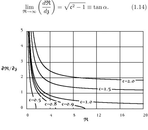
cR≥exp [−R]−1 +R, (1.13) where, from (1.12), the equality holds for stationary points, d_dR_z = 0. Figure 1.1 provides a graph of (1.12) for various values of the parameterc. Note that, forc¿ 1,

lim

R→∞

dR dz

=c2−₁≡_{tanα. (1.14)}

Figure 1.1: Graphs of d_dR_z versusRfor various values of cfrom equation (1.12). For cases where c <1, d_dR_z = 0 gives the radiusR_M of maximum girth. For c>1, the horizontal asymptote of dR

dz equals the tangent of the

half-angleαof the enveloping cone, as in (1.14).

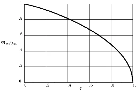
Numerical integration of (1.12), evaluated at the limit

dR

dz=0, enables one to calculate theRzMM versuscat

max-imum girth. The results are shown in Figure 1.2. In general, the solutions to (1.12) bear a striking re-semblance to the conic sections. For values c <1, the solutions are approximately elliptical, depicting crowns that are “pseudo-ellipsoidal”. The solutions are slightly broader near the vertices than their conic counterparts. For valuesc>1 , the solutions are hyperbolic depicting crowns that are “pseudo-hyperboloids “ (one sheet of the two-sheet variety). The asymptotes define the coni-cal appearance in this case. For c= 1, the “parabolic” case, the crown appears cylindrical with a rounded top. (Unlike the parabola, the derivative d_dR_z = 0 for largez.)

1.3

Experimental Results

Figure 1.2: Graph of RM

zM versus cfor the elliptic case,

c<1. From (1.12) , values of RM

zM where computed for

c= 0.0,0.2, . . . ,1.0. A smooth curve was drawn through these points.

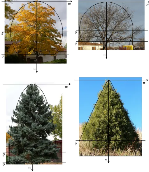
if necessary, and down-loaded into a True BASIC pro-gram designed to superimpose a computed profile over the tree. Examples of four such ”best fits” are shown in Figures 1.3 (posted at the end of Part 1). In my re-search, 33 trees and woody shrubs were thus studied. The trees chosen for inclusion in this report are not ex-ceptional; they were selected mainly to exemplify the various of tree shapes. Of course, only uncrowded, un-damaged, mature trees were included in the study. To minimize parallax, unobstructed views were required so as to obtain telephoto images.

The trees included in this report include two Honey-locustRobinia pseudoacacia, SprucePicea engelmannii, and Juniper Juniperus scopulorum. Superimposed on each image is the “best fit” theoretical profile matched by adjusting the constant c and the position of the leaf-line z_N. The “best fit” profiles were determined by “eye”. (A numerical scheme such as “least-squares” could have been used, but in this author’s opinion, such analysis is not warranted in this preliminary study with limited data.) Also shown on those figure for which c < 1, is the coordinates of maximum girth, z_M. The best-fit values of this analysis are given in Tab 1.1 to two significant figures of accuracy.

The leaf-line constant z_N was introduced originally to limit the range of numerical integration. However, this constant is somewhat diagnostic of tree shape for conifers. For the set of spruce trees studied, c ≈ 0.9, and moreover RN

zN ≈0.3. No analogous relationship was

observed among deciduous trees; contrarily, note the dif-ference in c values between the two honey-locust trees in Table 1. For trees with c > 1, the parameter z_N is particularly relevant to tree shape: the greater z_N, the

“sharper” the tree top.

The parameterb associated with the decrease in leaf density with distance in from branch-end can be eval-uated using the scaling relations R = bR and z = bz

introduced just above equation (1.12). The coordinate of maximum girth,Rm, is particularly convenient (when e<1) because it can be computed directly from (1.13) at equality.

The computed valuesb are generally higher than ex-pected: 1_b implies a “compensation point” where leaf density is decreased by 1_e ≈0.368 of its maximum value at branch-end. By measurement, in several cases, the actual distance 1_b is greater than that calculated and shown in Tab. 1.1.

1.4

Discussion and Summary

The approximate azimuthal symmetry common to most trees in this temperate latitude (Colorado) sug-gested to this author that growth and form progressas if ambient light alone is sufficient.. Building on this concept, and using the density of foliage as a proxy for the distribution of photosynthetic units, a theory was developed which determines the profile of a tree (crown) from optimization of the light gathering potential, i.e. the number of leaves available.

The theory predicts, reasonably well, the profile of trees: generally, trees with uniform distribution of fo-liage exhibit rounded crowns (such as with many de-ciduous tree); trees with their foliage concentrated near the outer stem-ends exhibit conical crowns (such as with many conifers). Mathematically, the calculus of varia-tions was used to find the profile (i.e. the radial branch length as a function of position along the main stem symmetry axis) which gave the maximum number of leaves (the integral of the leaf density) for a given size of tree (as measured by a fixed bounding surface area). A density-of-foliage function was introduced that held the stem-end leaf density constant, and allowed a fall-off of density inward toward the main stem or symmetry axis. An exponential density function was chosen which met these requirements.

The theory also predicts that the single parameter,

c (> 0) is sufficient to define the profile. Trees with

c < 1 have rounded profiles (c = 0 are circular); with

c > 1, conical. The profiles are qualitatively similar to the conic sections: Indeed, the terms elliptic, and hy-perbolicserve as appropriate bynames for the respective profiles, overlooking the sometimes significant quantita-tive differences.

The theory was compared with actual trees by super-imposing the computed profiles over the digital images of actual trees. Beyond adjusting for scale by settingz_N

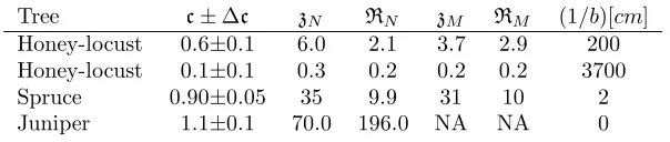
Tree c±Δc z_N R_N z_M R_M (1/b)[cm] Honey-locust 0.6±0.1 6.0 2.1 3.7 2.9 200 Honey-locust 0.1±0.1 0.3 0.2 0.2 0.2 3700 Spruce 0.90±0.05 35 9.9 31 10 2 Juniper 1.1±0.1 70.0 196.0 NA NA 0

Table 1.1: “Best fit” values of c and the associated values, z_N, R_N, z_M, R_M, and b. The uncertainty values±Δc indicate the range over whichccan be adjusted with less than 10% change in the values of the other parameters.

a good visual fit. I also found that, for trees for which

c < 1, the ratio RM

zN , where zM is the longitudinal

po-sition of maximum girth, is rather constant for a given species; this relationship was not investigate further in this study. In a similar manner, for conical trees, the setting of z_N adjusted for the roundedness of the tree apex, high settings ofz_N gave pointed apices.

The agreement between the distribution of leaves and the availability of light (which was the concern motivat-ing this study) was not determined because of my not having convenient way of measuring both leaf density and light intensity within the crown. I tried to determine leaf density by measuring the light passing through the foliage using a light meter-telescope combination, but this strategy was not successful.

It is well known that the tree-growth is controlled the four basic ingredients: light, water, carbon dioxide, and nutrients. The present study suggests that light alone is responsible for tree shape (although I admit that the connection of light to foliage was not well established in this study). But further evidence of this hypothesis follows from the observation that a tree with multiple main stems, or even a small group of trees growing very close together, produce a collective crown whose profile is similar to that of a single tree.

Part 2:

Branches

2.1

Introduction

This study is based on one simple but significant ob-servation: The cross-sectional area of a branch (or stem) entering a fork (in the direction of water transport) is less than the sum of the cross-sectional areas of the branches leaving that fork. To quantify this, I introduce the “bulking ratio”

γ≡ Area.of.branch.entering.fork

Areas.branches.leaving.fork (2.1)

All areas are measured outside of the swollen region (collar) of the fork. I made measurement on 128 forks on 21 different species of trees and tall shrubs, chosen opportunistically, in the vicinity of Denver, CO. To my surprise, the mean bulking ratio was less than one: in-deed,γav= 0.867 with standard deviation SDγ = 0.105.

The probability of this result if γtrue=0 is clearly in-finitesimal.

Moreover, and even more surprising to me, was a re-lationship betweenγand the angles between the outgo-ing branches: The angles between the out-going branches tended to increase withγ. The primary objective of this Part is to understand this relationship.

One might expect that the ratio of areas should beone considering both the continuity of venation across the fork and the strength required to support the weight-of-branch beyond the fork. In this latter regard, the cross-sectional area of a branch (or stem) at a given point is proportional to the load supported at that point. The constant of proportionality depends on the strength of the wood. (Specifically, the strength required depends on whether the wood at that point is under compression, tension, torsion, flexure, or some combination there of.) Strength is measured in units offorce per unit area. It is assumed that the swollen region of the fork is sufficiently small (in distances along the branches) that the load supported by the incoming branch is essentially the same as that supported by the sum of the outgoing branches.

2.2

Theory

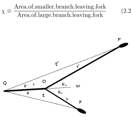
To simplify the analysis, considere a simple two-branched fork confined to a single plane; see Figure 2.1. The line QO represents the incoming branch; OP and OP’ the outgoing branches. The lines QO, OP, and

OPlie in a single plane. The ellipses at the ends of the outgoing branches represent terminal buds. The angle

ω = θ_ω+θ_ω is the only angle measured in the field; the other angles as well as the lengths r,s, s,t, andt

are used in the analysis. A fork in which the branches

OP andOPlie in a different plane from that ofQOand

The fork, as introduced, concerns terminal twigs. The analysis, however, reduces to a consideration of the fork in the neighborhood of point O, at which only the ar-eas of the incoming and outgoing branches are involved. Because it seems reasonable (and not contradicted by limited observations) that a fork maintains its geometry from inception to maturity, the analysis is assumed valid for all simple forks.

My strategy is to assume some reasonable model for the cross-sectional area of a branch in terms of position along the branch, then, given the positions of the posi-tionsQ,P, andP, find the pointO that minimizes the volume of tissue in that region of fork. The points P,

P, andQ are merely reference points which, it will be shown, drop out in the final analysis.

As the two branches are usually of different sizes, I introduce thebranching ratio χ.

χ≡ Area.of.smaller.branch.leaving.fork

Area.of.large.branch.leaving.fork (2.2)

Figure 2.1: The geometry associated with the analysis of the fork. PointO locates the intersection of the central lines of the branches. PointQis a point on the center-line of the incoming branch arbitrarily close to point

O. PointsP andP on the center-lines of the out-going branches denote positions of equal branch area; P and

P are arbitrarily close to pointO.

The volumeV of a branch segment (with no interven-ing side branches) between pointsaandbcan be written as the integral of the branch area A[x] in terms of the distancexis along the branch,

V = _abA[x]dx. It is convenient to write the area as the product A[x] = A0g[x] such that g[0] = 1; it is reasonable to think ofg[x] as a monotonically increasing function ofx. In the case of constant elastic modulus,

g[x] would be exponential: g[x] = exp[bx], where x is measured inward/downward. Choosing pointsP andP

(terminal branch ends) as the starting points along the two outgoing segmentsOP andOP, their volumes are, respectively,

V_s=A0

s

0

g[x]dx=A0G[s], (2.3a)

V_s =A0

s

0

g[x]dx=A0G[s], (2.3b)

where capitalGrefers to the integralg. Here,G[x] must be differentiable, dG

dx =g[x]. I assume that the area of

the branch at pointP is the same as that atP!

The volume of the segment QO is given by

V_r=A1

r

0

g[x]dx=A1G[r], (2.3c)

where A1 is the area of the incoming branch measured at pointO. From the definition of the bulking constant (2.1), one can write

A1=γ(As+As) =γA0(g[s] +g[s]). (2.4)

Thus, the expression for the volumeV_rcan be written

V_r=A1

_r

0

g[x]dx=γA0(g[s] +g[s])G[r].

The total volume of the forkV =V s+V s+V r, where the volume of the swollen part of the fork is neglected. From equations (2.3a, 2.3b 2.3c),

V =A0G[s] +A0G[s] +γA0(g[s] +g[s])G[r]. (2.5)

The distancesandscan be related tor,θandr,θby means of the cosine theorem as applied to the triangles of Figure 1:

s2=t2+r2−2rtcosθ, (2.6a)

s2=t+r2−2rtcosθ. (2.6b)

recalling that dG_dx =g[x]:

∂V ∂r =A0

g[s]∂s

∂r +g[s _]∂s

∂r +γ(g[s] +g[s

_])g[r]+

+γ dg ds+ ∂s ∂r + dg ds ∂s ∂r

G[r]

, (2.7a)

∂V ∂θ =A0

g[s]∂s

∂θ +g[s _]∂s ∂θ+ +γ dg ds ∂s ∂θ+ dg ds ∂s ∂θ

G[r]

. (2.7b)

The partial derivatives ofsands, here, can be calcu-lated from the cosine theorems (2.6a, 2.6b); again, with reference to Figure 2.1,

∂s ∂r =

r−tcosθ

s =−cosθω, ∂s ∂θ =

rtsinθ

s =rsinθω,

(2.8a)

∂s ∂r =

r−tcosθ

s =−cosθ

ω,

∂s ∂θ =

rtsinθ

s =rsinθ

ω.

(2.8b)

Consider (2.7a, 2.7b) in the limit of very short in-coming branch, i.e. r → 0; in this limit,g[r] → 1 and

G[r]→0. Equations (2.7a, 2.7b), with (2.8a, 2.8b), can be written,

∂V

∂r =A0(g[s](−cosθω) +g[s

_](−cosθ

ω)+

+γ(g[s] +g[s])), (2.9a)

∂V

∂r =A0(g[s] sinθω−g[s _{] sinθ}

ω)r. (2.9b)

Ignoring the trivial solution r = 0 in (2.9b), setting

g[s]+χg[s], (following (2.2), and recognizing thatA0g[s] andA0g[s] are the areas of the outgoing branches near point O, factoring out the term g[s], and setting the derivatives equal to zero , one finds:

γ(χ+ 1)−χcosθ_ω−cosθ_ω= 0, (2.10a)

χsinθ_ω−sinθ_ω= 0. (2.10b)

Equations (2.10b) can be solved simultaneously forθ_ω, andθ_ω. By squaring and converting the sines to cosines, and performing the required algebra:

cosθ_ω= 1 2χ

(1 +χ)γ−(1−χ)1

γ

, (2.11a)

cosθ_ω= 1 2χ

(1 +χ)γ−(1−χ)1

γ

. (2.11b)

Also, with reference to Figure 2.1,

ω=θ_ω+θ_ω. (2.12)

Equations (2.11a, 2.11b) and (2.12) can be solved nu-merically to giveω as a function ofγ andχ. Figure 2.2 provides graphs of ω versus χ for several appropriate values ofγ. Note the limits:

• For γ = 1 (no area increase across the fork), θ =

θ = 0◦, thusω = 0◦. In this case there would be no branching at all; every leaf would find itself on a lone stem originating at the ground.

• For χ = 1 (equal size branches leaving the fork), equations (2.11a, 2.11b) yield θ = θ = cos−1_γ, thus, from (2.12),

ω= 2 cos−1γ. (2.13) This formula (by inspection of Figure 2.2) holds to fair approximation for branching ratiosχ >0.6.

• There is a minimum branching ratioχmin for any given bulking ratioγ,

χmin= 1−γ

1 +γ. (2.14)

Figure 2.2: A graph of the branching angle ω versus the branching ratio χ for four different values of the bulking ratio γ. The equal-branch (χ = 1) solution,

ω= 2 cos−1γ, holds approximately forχ >0.6.

Equation (2.11a) shows that the angle θ_ω increases with decreasingχ, while (2.11b) shows thatθ_ω decreases with decreasing χ, both as expected. Moreover, as χ

ratio γ must approach one (even branching), again as expected.

For the case of small χ, branching angles ω > 90◦ is curious; it suggests that a twig can be reflexed i.e. angled back on its incoming branch. Either this is an unrealistic artifact of the theory, or perhaps it allows for the unusual case that ample light is found in the interior regions of the tree promoting reflexed behavior? It is this author’s intention to pursue this matter.

Consider a branch segment as shown in Figure 2.1 with the incoming branch starting at pointQ, the opti-mized branch point atO, and the outgoing branch ends at pointsP andP. From Figure 2.2, the volumeV (as given in (2.5)) is a monotonically increasing function of the bulking ratio γ, for given value of χ. This implies that less volume of wood is needed to connect pointQ

withP andPif the bulking up is low; thus, the branch-ing angle high.

2.3

Field Measurements

Prior to conducting the theoretical work described in the preceding section, I measured the cross-sectional ar-eas of the incoming and outgoing branches of 124 forks representing 21 species of trees and tall shrubs near Den-ver, Colorado. In terms of the ratio bulking ratio defined in (2.1), I found that, γav±Δγ= 0.877±0.105, where 0.105 is the standard deviation. The probability that the population meanγ∗_av= 1, given my data, is infinitesimal. The only requirement I imposed on the specimens was that all the branches be relatively round so that the cir-cumferencesquaredwould serve as a proxy for area. (To measure the circumferences I used a flexible measuring tape wrapped just beyond the swollen region of the fork.) Fortunately, 103 of my earlier measurements were “sim-ple” forks for which I had also measured (with a large two-armed protractor) the branching angle ω. It was surprising to me, incidentally, how few forks were of this simple two-branched variety. Most forks involved three or more out-going branches, some forks were within the swollen zone of neighboring forks, and some forks were simply not round enough or too disfigured to qualify. I measured forks with circumferences ranging from a few millimeters to meters. Where possible, I would select forks on recently dead branches without bark so as to focus attention on supportive tissue alone.

I did not attempt to collect a scientifically random sample; I just selected trees and shrubs of as many dif-ferent species which were convenient for me to measure. I did not distinguish between forks in branches, branches off the main stem, or bifurcations of the main stem. Be-cause I am interested in “universal” properties of woody plants, I sampled as broad a representation of species and sizes as possible. My data set is not large enough

to distinguish quantitatively agreement within species or differences between species, although I have noted some such regularities.

Figure 2.3 shows a graph of branching angleω versus bulking ratioγfor forks with out-going branch area ratio

χ > 0.6. Forks with χ > 0.6 (somewhat equally sized out-going branches) obey, approximately, (2.13).) Here, 76 of the 103 specimens meet this criterion.

Figure 2.3: A graph of the measured values of the branching ratioωversus the bulking ratioγfor 76 speci-men of trees and shrubs of branching ratioχ >0.6. The data is represented by ellipses whose dimensions gives the average measurement error. The smooth curve gives the theoretical dependence ω= 2 cos−1_γ.

The trend of the data is in agreement with the theory, but the spread is too great to make any meaningful com-parison with theory. This spread might well be due to environmental factors affecting the forking. Moreover, with regard to theory, the minimum in volume, from which the theoretical branching angle is determined, is both broad and shallow. This means that there is little penalty in tree resource if the optimum branching angle is not achieved. (Perhaps the curve ofωversusγshould be drawn with a broad pen.)

2.4

Discussion and Summary

The “bulking up” of branches, as measured byγseems to be an empirical fact, at least for the vast majority of trees and woody shrubs in this temperate zone. Like-wise, the increase in branching angleω with increasing

γ is strongly suggested. It is reasonable to believe that branching angle is genetically controlled; my measure-ments on young sprouts (not included in this report) show significant variation around the average. Perhaps those branches that are favorably oriented have a better chance of surviving to maturity and being measured by a curious researcher.

The value of this study to conventional tree archi-tecture is in the constraints it imposes on branching. But with respect to understanding the morphological implications of genetic control, this work could provide a theoretical framework. As the branching angles were measured on relatively mature trees, environmental fac-tors have had time to operate. Perhaps sectioning more branches longitudinally (as advocated by Shigo (1994)) through the forks and measuring the initial branching angles at the core (pointO in Fig. 2.1) would be more appropriate.

This author is under no illusion that the theory pre-sented here provides the primary explanation of fork morphology. There is, however, strong empirical evi-dence that “bulking up” occurs and that branching an-gleω is related to the bulking ratioγ . The minimum volume theory presented here provides a plausible ex-planation for that relationship.

Part 3:

Trunk

3.1

Introduction

The objective of this Part is to exploit the concepts of the first two Parts of the report to further test of the validity of those ideas. In particular, the shape of the main stem (i.e. the cross-sectional area of the main stem as a function of position) is deduced from the pro-file of the tree and the angle of branching off the main stem. This study is limited to trees with a single main stem whose primary branches make an angle of 90 de-gree with the trunk. The theoretical results, then, are compared with actual measurements on three represen-tative trees: a douglas-fir (Pseudotseuga menziesii), a juniper (Juniperus scopulorum), and an aspen (Populus

tremuloides). As this study is intended merely as a check on the preceding studies, no effort was made to include a greater number of individuals or a broader variety of species. (Trees featuring both a single main stem and perpendicular branching limited the number of species available, especially among deciduous trees.)

3.2

Mathematical Set-up

The average behavior of branches off the main stem can be modeled as a distribution of infinitesi-mal branches, each originating at the axis of the main stem, projecting perpendicular from the axis to a ter-minal point at coordinate r, θ, z, where one can imag-ine an infinitesimal leaf. Assuming exponential increase of branch area towards the main stem, and a terminal branch area proportional to the density of leaves at that point, the element of cross-sectional aread3aat the main stem (approximated asr= 0) can be written

d3a∝exp[αr] exp [−b(R[z]−r)]rdrdθdz, (3.1) whereR[z] gives the profile as defined in Part 1;αand

b are constants as defined previously. Expression (3.1) can be integrated first overθ (the partial integral being 2π) and then overrto yield.

da= Cb (α+b)2

((α+b)R−1) exp[αR] +

+ exp[−bR]dz, (3.2a)

whereR=R[z] andC is a constant.

With the introduction of the dimensionless variables defined above Equation (1.12): (3.2a) can be written

da=C 1

(1 +e)2

((1 +e)R−1) exp[eR] +

+ exp[−R]dz, (3.2b)

where, again,z=bz,R=bR, ande= α_b, a=b2a, and R=R[z].

As applied to the fork formed by the main stem and the infinitesimal branch intersecting at a length element

dz, the bulking ratioγ (equation (2.1) is given by

γ=A[z+dz]

A[z] +da=

A[z] +dA_dzdz

A[z] +da

dzdz

= 1−dγ, (3.3)

where

dγ= 1

A

da dz −

dA dz

Tree c (1/b)[cm] R[z] e C √variance Juniper 1.11 2 0.5z 0.012 6.6*10−3 _0.02 Aspen 0.88 25 0.3646z−z2 _{0.04 1.0*10}−4 _0.04 Douglas-fir 0.99 3.5 .0932160z−z2 _{0 1.15*10}−2 _0.02

Table 3.1: Best fit values of the profile parameters: c and 1_b, the quadratic equation for the conic approximation: R[z], the trunk parameters: e, C, and the square-root of the variance: √variance. (In the analysis, the parameters e, C were adjusted to render the variance a minimum.) The √variance has been normalized by dividing by the maximum trunk area to render the values comparable.

In Part 2, the bulking ratioγwas shown to be a func-tion of both the branching ratio χ and the branching angle ω. If dγ in (3.4) is replaced by _dχdγdχ and rear-ranged, then

dA dz =

1−dγ

dχ

da dz;

thus,

A[z] =

_z

0

1−dγ

dχ

da[z]

dz dz

_{. (3.5a)}

In dimensionless variables,

U[z] =

z

0

1− dγ

dχ

da[z]

dz dz

_{. (3.5b)}

The branching ratiodχis given by

dχ= da

A. (3.6)

Taking χ as its average over an element of distance Δz, and writing Δa= da_dzΔz. then,

χ= 1

A da

dzΔz. (3.7a)

In dimensionless variables,

χ= 1 U

da

dzΔz. (3.7b)

For the purpose of this Part, the branching angle is set at 90◦ (ω= π

2). As an explicit expression forγas a function ofχis not available, anapproximateexpression was derived in the form of the third degree polynomial:

γ= 1−χ+ (3γ1−1)χ2−(2γ1−1)χ3, (3.8) where γ1 is the value of γ at χ = 1; in general, from (2.13),

γ1= cos

_ω

2

. (3.9)

Ifω= π₂, thenγ1=√1₂. The coefficients of (3.8) were determined by first considering that atχ= 0,γ= 1; and atχ= 1,γ=γ1. Then, following (2.11, 2.12), the par-tial derivative (∂γ_∂χ)_ω (i.e. ω is held constant at π₂) was evaluated at its limiting values; at χ= 0, (∂γ

∂χ)ω =−1;

and at χ = 1, (∂γ_∂χ)_ω = 0. The gains in both conve-nience and insight by using the approximation contained in (3.8) are significant.

The cross-sectional area A[z] of the trunk as a func-tion of distance from the tree top is given by (3.5a); da_dz by (3.2). Now, dγ_dχis just the derivative of (3.8), wherein

χcan be expressed in terms of z by (3.7a). (For working purposes, I carried out this analysis using the dimen-sionless variables, the (b) equations.)

Equations (3.5) for area requires knowledge ofχfrom (3.7), which in turn requires knowledge of area. Here, the following iterative procedure was used: First, set the derivative _dχdγ = 0 (this is equivalent to setting γ = 1, no bulking-up). Then (3.5) can be integrated to yield a first approximation of area. Substitution of this expres-sion for area into (3.7) givesχ[z]. Next, substitution of

χ[z] into the derivative of (3.8) yields dγ_dχ as a function ofz, which, in turn, can be substituted back into the in-tegral of (3.5) to produce a newA[z]. This process can be repeated as often as needed; however, convergence is fast.

3.3

Field Measurements and Analysis

theo-Figure 3.1: Calculated values of areasA[z] andvariance between the measured and theoretical areas for each of the three cases (a-top; b-middle; c-bottom.)

retical areas for each of the three cases was calculated.

3.4

Discussion and Summary of Part 3

In Part 3, the concepts of Parts 1 and Part 2 are tested by combining them to predict the cross-sectional area of the trunk of a tree with a single main stem and horizontal branches. No new concepts are introduced. To further simplify the analysis, conic approximations (as introduced in Part 1) are used to represent the profile

R=R[z].

The data is well matched by the theory as shown in the Figure 3.1 wherein the two free parameters,e,C. are adjusted to find the (unique, I believe) minimum in the variance. As in other aspects of this study, the minimum is broad with respect to the two parameters. Although the results of this Part support the concepts of Parts 1 and 2, it must be cautioned that other two parameter models (quadratic) can also be adjusted to fit the data. The dotted curve in Figure 3.1c gives the trunk area if the trunk were a perfect cone with base near z = 700cm. This curve is presented because a trunk is often modeled as a cone in estimating the volume of wood, an approximation which seems to under-estimates the volume, as would be prudent.

General Summary

The results of this study does not constitute a tree model in the manner of the pipe models of (Shi-nozaka et al. 1964a,b), (Valentine 1985), (Rennolls 1992), etc., but it presents theoretical considerations rel-evant to such whole-tree models.

The basic assumption here is that the architecture of the tree will be such as to minimize plant tissue while providing for the tree’s needs. In Part 1, the overall shape of trees is considered, with an eye to the distribu-tion of leaves (photosynthetic units); in Part 2, branch-ing is considered, with the angle of branchbranch-ing of primary interest. The mode of investigation is mathematical, with the calculus of variation the central tool. The mod-els developed are checked against field measurements. Although the agreement between theory and measure-ment is reasonable it falls far short of “validating” the models. Only the most obvious of predictions are tested. The possible taxonomic connections suggested by the models are barely touched upon.

Although it is this author’s intention to continue the field work, there are problems in my so-doing: Ac-cess to the canopies of mature trees is difficult in most cases. Finding trees that are more-or-less undeformed by crowding, damage, or disease is often an issue; most trees in an open forest are suitable for my purposes, but obtaining telephoto images of individual trees is diffi-cult And most challenging is finding ways to easily and cheaply measure leaf density; direct leaf counting is un-duly tedious.

considered here are important in tree morphology. How-ever, the agreement between theory and measurement is sufficiently good to suggest that the ideas presented here be considered reasonable hypotheses.

Acknowledgements

I am especially pleased to thank my wife, Loraine Yeatts, for help in all aspects of this work: she did nearly all the photography, assisted with most of the field work, and provided expertise on all botanical matters. My thanks also to Priscilla Spears (who also contributed some photos of trees), Rick Brune, and Carol English for helpful discussions. I am very much indebted to the editors of MCFNS and to the reviewers of this paper for their encouragement and further recommendations on the literature.

References

Bell, Adrian D. and Alan Bryan. 1991. Plant Form: An Illustrated Guide to Plant Morphology. Oxford. 341p.

Berninger, Frank, Lluis Coll, Petteri Vanninen, Annikki Makela, Sari Palmroth, and Eero Nikinmaa. 2005. Ef-fects of tree size and position in pipe model ratios in Scots pine. Can. J. For. Res. 35:1294-1304.

Emerson, Robert. 1929. Photosynthesis as a function of light intensity and of temperature with different con-centrations of chlorophyll. Journal of General Physi-ology 12(5): 623-639.

Hall, D. O. and K. K. Rao. 1999. Photosynthesis, Sixth Edition. Cambridge. 214p.

Horn, Henry S. 1971.Trees, Princeton. 144p.

Kantola, Anu, Harri Makinen, and Annikki Makela. 2007. Stem form and branchiness of Norway spruce as a sawn timber - Predicted by a process based model. Forest Ecology and Management 241:209-222.

Makela, Annikki. 2002. Derivation of stem taper from pipe theory in a carbon balance framework. Tree Phys-iology 22:891-905.

Makela, Annikki and Harry Valentine. 2006. Crown Ra-tio Influences Allometric Scaling in Trees. Ecology 87:2967-2972.

Mitchell, Kenneth J. 1975a. Dynamic and simulated yield of Douglas-fir. For. Sci. Monogr. 21(4):1-40.

Mitchell, Kenneth J. 1975b. Stand description and growth simulation from low-level stereo photos of tree crowns. J. For., January:12-17.

Rennolls, Keith. 1994. Pipe-model theory of stem-profile development. Forest Ecology and Management. 69:41-55.

Savage, V. M., L. P. Bentleyc; B. J. Enquistb, J. S. Sper-ryd, D. D. Smith, P. B. Reiche, and E. I. von Allmend. 2010. Hydraulic trade-offs and space filling enable bet-ter predictions of vascular structure and function in plants. PNAS 107(107) :22722-22727.

Shigo, Alex L. 1994. Tree Anatomy, Shigo and Trees, Associates. 104p.

Shinozaki, K., K. Yoda, K. Hozumi, and T. Kira (1964) A quantitative analysis of plant form: the pipe model theory. I. basic analyses. Japanese Journal of Ecology 14:97-105.

Tausch, Robin J. 2009. A Structurally Based Analytic Model for Estimation of Biomass and Fuel Loads of Woodland Trees. Natural Resource Modeling, 22(4): 463-488.

Thomas, Peter. 2000. Trees: Their Natural History. Cambridge. 286p.

Tiangco, Peter N. and Bruce C. Forester. 2000. Development of trunk-canopy biomass and mor-phology indicies from quadpolarized radar. URL: http://gisdevelopment.net/aars/acrs/2000/ts12/ ts1203pf.htm

Valentine, Harry. 1985. Tree growth models:Derivations employing the pipe-model theory. J. theor. Biol. 117: 579-585.

Valentine, Harry T., Anthony R. Ludlow, and George M. Furnival. 1994. Modeling crown rise in even-aged stands of Sitka spruce or loblolly pine. Forest Ecology and Management 69:189-197.

Valentine, Harry and Annikki Makela. 2005. Bridging process-based and empirical approaches to modeling treee growth. Tree Physiology 25:769-779.

Wang, Mingliang and Kieth Rennolls. 2007. Bivariate Distribution Modeling with Tree Diameter and Height Data. Forest Science 53:16-24.

Waring, R. H., P. E. Schroeder, and R. Owen. 1982. Applications of pipe model theory to predict canopy leaf area. Can. J. For. Res. 12:556-560.