(DOI: 10.24874/jsscm.2018.12.01.07)
Modelling of the Femoral Fracture Under Dynamic Loading
A.Moulgada1,*, M.E.Zagane1,2, A.Benouis2,A.Sahli2,, M.Cherfi2 and S.Benbarek2
1 University Ibn Khaldoun, BP 78, City Zaaroura, Tiaret 14000, Algeria e-mail:[email protected]
2 Laboratory of Mechanics, Physics of Materials. University of Sidi Bel Abbes, 22000, Algeria e-mail:[email protected]; [email protected] ; [email protected];
[email protected]; [email protected] *corresponding author
Abstract
Bone is a living material with a complex hierarchical structure that gives it remarkable mechanical properties. The bone undergoes constant mechanical and physiological stress, so its quality and its resistance to fracture evolve constantly over time through the process of bone remodelling. Bone quality is not only defined by bone mineral density but also by mechanical properties as well as micro architecture. The aim of this work is to model the fracture of the femur bone under a quasi-static and dynamic solicitation in order to create a digital model simulating the fractures of this element due to an accident. This modelling will contribute to improve the design of the means of transport to bring a better security to the passages. To achieve this goal, the modelling by the finite element method is performed to study the mechanical behaviour of bone structure and predict femur fractures.
Keywords: Biomechanics, finite element, femur, damage, fracture, dynamic
1. Introduction
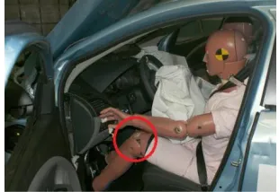
modelling using the Johnson-Cook damage criterion, the geometric model includes all the coxofemoral complex, we simulated the fracture of the bone under a loading similar to that of a car accident, the driver is seated (Fig.1), the impact is a rectangular plate associated with a mass corresponding to the human weight of 80 kg and a variable speed of (7m/s; 14m/s and 22 m/s).
The aim in this simulation is to detect the places in the bone that can be fractured and also to study the effect of the shock velocity on the type of fracture, so our analysis will allow the car designers to better understand the phenomenon accident and improve designs to have maximum safety at the edge of cars, knowing that the international protection system is also designed to effectively protect the driver up to an impact speed of 17.77 m/s (Burr et al.1988). Numerous criteria have been developed for the initiation of ductile failure in the nonlinear domain of metals.
Fig. 1. Frontal shock test of a vehicle according to (Jonathan et al. 2008)
2. Scenario of the force exerted on the femur during the shock
Fig. 2, illustrates the load associated with fractures and dislocations in a frontal shock. The force exerted on the knees is transmitted through the distal parts and in the middle of the femur in the hip joint. A frontal collision begins with an acceleration caused by the contact between the front end of the vehicle and an object such as another vehicle or a tree.
Fig. 2. Illustration of the scenario of the injury in a vehicle crash
3. Behavior of the bone under dynamic loading
3.1 Laws of Johnson-Cook
often adaptations of behavioral laws of non-biological materials such as steels, composites, foams, etc.
This law is very widespread and was proposed in 1983 by (Johnson and Cook 1983); since then, it has been used with variants in many cases (Rule, and Jones 1998, Gavrus et al. 2003).
1 ln
0
n
b c
y p
(1)
σy, b, n and c are the constants defining the material (Table1): σy is yield stress, b is the rate of work hardening, n: the exponent of work hardening, c: the coefficient of strain rate and with έ0 the initial deformation speed. The first factor of the expression gives the dependence of the elastic limit on the nonlinear deformation; the second factor represents the sensitivity to the speed of deformation. This approach does not take into account the effects due to the history of the strain speed. This model is a purely empirical law, it has been very successful because of its simplicity and the wide availability of parameters for different materials, in addition, these parameters can be obtained by a small number of experiments, more complex models can provide a more accurate description of the behaviour of the material, but these more complex patterns are not always readily integrable into commercial calculation codes via user routines. The disadvantage of this model is the imposed form of the work hardening of the material (power type).
The choice of ε0 influences the value of the parameter c during the process of identification of the stresses, one obtains a deferential value for c if the value of ε0 is modified, there is no unanimity in the literature concerning the choice of ε0, but a value of ε0 = 1s-1 is commonly used. The following relationship has been assumed to model the behaviour of the material, which is similar to the Johnson-Cook equation, this law has often been used to represent the behaviour of bone (Meyer and Kleponis 2001). This is a simple model for modelling the behaviour of metals at large deformations, for strain rates, and used to describe the behaviour of materials subjected to dynamic loading.
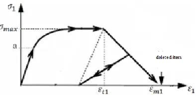
The law is linear elastic up to the limit of elasticity, fig. 3 show the stress-strain curve in the non-linear part, when the maximum deformation is reached, the element is deleted.
Fig. 3. Johnson-Cook law used to represent the structural behaviour of the bone
The Johnson-Cook Damage Law is frequently used to analyse bone structures under dynamic loading. This hardening law is generally premised in EF codes, including ABAQUS / Explicit. The material exhibits a linear elastic behaviour before undergoing a damage phase from a certain damage threshold fixed according to the mechanical characteristics of the material.
v
1 2; 1 2
1 1
1 1
1 1
v
E E
d E d E
(2)
v
2 1; 2 1
2 2
v
E E E E
(3)
1212 1 1 d G
(4)
1
1 2 1 2
1 1
v
1 1 v
E d
d
1
1
2
1 2
1
1 12
12 1 1 1
1 E d v d v d G
(5)
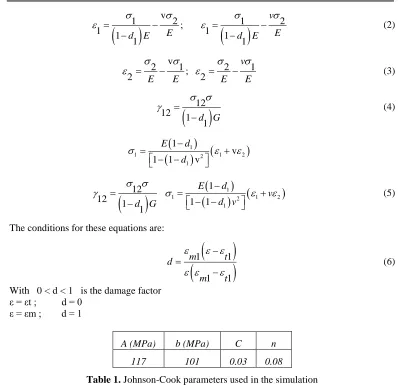
The conditions for these equations are:
1 1 11
m t d m t
(6)
With 0 < d < 1 is the damage factor ε = εt ; d = 0
ε = εm ; d = 1
A (MPa) b (MPa) C n
117 101 0.03 0.08
Table 1. Johnson-Cook parameters used in the simulation
4. Modelling
Obtaining the patient's solid 3D model of the femur consist to taking images of the region of interest using a medical imaging technique (CT-scan). The thickness of each slice is from 1 mm for the proximal part to the small trochanter, and from 8 mm from the small trochanter to the most distal part of the diaphysis, two regions can be distinguished (cortical bone and cancellous bone). The 3D reconstruction of the two regions is done separately (Hambli et al. 2013).
4.1 Assembly
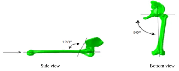
adduction) of the femur has been fixed such that a line connecting the midpoint of the femoral condyles to the hip and perpendicular to a line connecting the left hip centers, where the hip joint center was estimated by palpation of the head of the femur, the sacroiliac joint was modeled as bound surfaces, the sacroiliac joint was entirely fixed, while the pubic joint was greeted in sagittal plane; the boundary conditions are considered representative of anatomical configuration (fig 5) (Pauwels 1976), therefore, three parametric frontal impact simulations were performed to find the different fracture zones.
Side view Bottom view
Fig. 4. Femur-pelvis angles used in model simulation
The femoral mid distal to the head axis is perpendicular to the coronal plane of the pelvis, and the thigh-pelvis angle has been positioned in a sitting position in the car that refers to 120 ° between the major axis of the femur and the plane defined by the anterior superior iliac spines and the pubic symphysis (Benbarek et al. 2007).
4.1 Mechanical properties of the model
The mechanical properties of materials are taken from previous studies, for cortical and cancellous bone were defined as isotropic material (Table 2) (Schneider et al. 1983, Nerubay et al. 1973), the femur was considered a homogeneous and isotropic material, with distinct properties for the cortical and spongy bone, the hip being considered as a rigid material.
Materials E (MPa) υ σy (MPa) εy Ρ (kg/m3)
Cortical bone 17000 0.3 117 3.3 2000 Concellous bone 600 0.3 4.5 0.65 0.45
Table 2. Elastic properties of the isotropic bone
4.2 Boundary conditions
Impact
Fig. 5. Applied boundary conditions and the configuration of the impact model
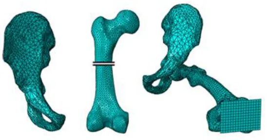
4.3 Mesh
Fig.6, shows the mesh used around both ends of the crack, reliable results requires a fine mesh, for it was used a type of mesh with C3D4 tetrahedral elements (150000) for a best approximation and optimal convergence of results.
Fig. 6. Meshing adapted to the model
The technique and the method used for the fracture of the bone called "deleted element" when the damage parameter reaches a critical value of damage factor is less than one, the mechanical contribution element to the stiffness matrix is set to zero.
The element is removed if a layer of the element reaches the deformation of the tensile fracture; affected elements were applied to simulate the process of progressive fracturing of the bone (Ural and Vashishth 2007).
5. Results and discussion
5.1 Distribution of equivalent stresses in the bone during impact
(7m / s, 14m / s and 22m / s), we note the distribution of the constraints for three distinct moments of impact which are: 0.15ms, 0.25ms and 0.40ms.
0.15ms 0.25ms 0.40ms
7 m/s
14 m/s
22 m/s
Fig .7. Distribution of the equivalent Von Mises stress [MPa] in the femur for the three impacts velocities
Fig.7 shows the variations of the equivalent stresses in the whole structure of the femoral cortical bone at different impact velocities (7m/s; 14m/s and 22 m/s), in the first moment of impact, we notice that the distal part is that which receives the first load of the impact, after the femoral neck which is then the most solicited, while the diaphysis supports only weak constraints. The stresses in the bone remain relatively small to the stress of the bone fracture, so from the first moments of impact, we can support this load, and finally the impact causes constraints that are raised at the level of the distal epiphysis and focus at the level of femoral neck at (t = 0.4ms).
5.1 Simulation of femur fracture under dynamic loading
The implementation of the failure criterion previously described in the Abaqus software allows us to visualize the fracture of the femur during the impact; the following fig. shows the fractures of the femur for different speeds and for different instants of impact, to simplify the calculations; the bone is supposed to be homogeneous, isotropic and linear. The results show that the variation of the impact velocity generates a variety of injuries to the femoral neck, the increase in impact velocities leads to different types of fractures, always the fracture begins with fracturing of the bone, then if the speed increases, the rupture ends by fragmentation.
In the first case (7 m / s), the simulation shows that, from the first moment of impact, the fracture is initiated in the neck of the femur near the head of the femur, then after 10 ms of the impact, the fracture always spreads near the head of the femur to reach the middle of the femoral neck, after 25 ms the fracture begins to deviate on the middle of the neck of the femur, these are due to the rotation of the head of the femur as it begins to take off from the femur; finally, the fracture continues vertically to reach the end of the free femur.
For this type of impact (low speed), the simulation gives us a fracture of the femoral neck and not its fragmentation, these results is comparable to that found under static loading, so the bone this fracture under quasi-static loads. If we increase the impact velocity (14 m/s), the femoral neck begins to fracture first in the area close to the greater trochanter, as the impact progresses, we note that the collar begins to fragment on its lower part; finally impact, the femoral head (or almost) is detached from the femur, this type of impact causes rupture of the femoral head with fragmentation of the cervix.
As final results of this analysis, the low speeds lead to a fracture of the bone more or less recoverable by immobilization of the bone and subsequently the bone reconstitution which makes it possible to resume the articulation, for high shock speeds the reconstruction of the joint can only be done by replacing an artificial joint; the speed of the shock destroys a part of the bone substance that cannot be recovered, so always, we must drive at low speeds and safer to predict minimal damage better than driving at high speeds.
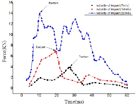
In order to detect the exact moment of the fracture during the shock, we measured the inertial force acting on the element during the whole shock time, the element is chosen in such a way that it undergoes the fracture itself ; the collected data are given in Fig. 9.
Fig. 9. Fracture time was determined from Force Stories for applied impact velocity (7m/s; 14m/s and 22 m/s)
Fig. 9 clearly shows that the higher the shock velocity, the greater the force, during the first moments of the shock (for all the calculated speeds), the force increases until reaching a maximum value, it is at this moment that the fracture begins, then the force decreases during a fraction of the time of the shock, this decrease. is the result of the passage of the fracture on the element concerned which undergoes strong shock before yielding, then it becomes the free edge of the front of the fracture and therefore it becomes free from any solicitation, after that, the force resumes its ascension that is to say that the force is re-exerted on this element, this is due to the position of the fracture which is far from the element and it undergoes stresses since the fractured part turns and tends these lips (the stressed element is part of the lips of the fracture); finally, we notice that the shock and after reaching its maximum, the latter begins to dissipate and the stresses begin to relax because they have been absorbed elastically and thus the shock stops, which explains that the force attenuates and tends to zero.
5.2 Validation of the digital model
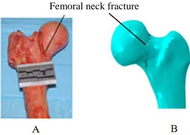
Femoral neck fracture
Fig.10. Comparison of the fracture location of the simulation (B) with the experimental results (A)
We simulated the impact on the femur by reproducing the same test conditions of Rupp et al. (2002). We have obtained a fracture of the femoral neck similar to that found by this author, the fig. shows a very great similarity between our numerical model and the experimental model of Rupp et al. so we can say that our digital model is validated and can be used to predict fractures during different types of accidents.
5.Conclusion
The fractures of the femur are the main causes of hospitalization in orthopedic surgery worldwide. In this study; a three-dimensional finite element analysis is carried out to study the phenomenon of cortical bone fracture of the femur under dynamic loading, different types of behaviour of the cortical bone have been analysed; The results obtained make it possible to deduce the following results:
Our numerical model accurately predicts the location of fracturing of the bone, which has been confirmed by comparing our numerical model with experimental work and giving a great similarity.
Our results allow us to say that Johnson-Cook's law simulates femur fracture in a precise way; this model of damage by its simplicity, allows modelling the dynamic behaviour of materials for large deformations and for different strain rates.
Stresses in the femur change during the duration of the impact, at the first moments of the impact, the stresses are concentrated in the contact zone with the impact (the plate), as the impact progresses, the highest stresses move from the epiphysis to the femoral neck through the diaphysis, at the end of the shock, all the load is concentrated in the femoral neck, which results in a rupture of the latter, the Shock velocity greatly affects the state and distribution of stresses in the femur.
The impact velocity gives different types of femoral fracture, low speeds (7 m/s and 14 m/s) give femoral neck cracking, and for high speeds (22 m/s and more) give a complete rupture with displacement of the femoral neck.
References
Benbarek S, Bouiadjra B Bachir, Achour T, Belhouari M, Serier B (2007). Finite element analysis of the behaviour of crack emanating from microvoid in cement of reconstructed acetabulum, Materials Science and Engineering: a, Volume 457pages 385-391.
Burr DB, Schaffler MB, and Frederickson RG (1988). Composition of the cement line and its possible mechanical role as a local interface in human compact bone. Journal of Biomechanics, 21(11): 939-945.
Cummings SR, Melton LJ (2002). Epidemiology and outcomes of osteoporotic fractures. The Lancet 359(9319): 1761.
Cooper C, Campion G, Melton LJ (1992). Hip fractures in the elderly: a world-wide projection. Osteoporos Int 2: 3rd 285.
Gullberg B, Johnell O, Kanis JA (1997). World-wide projections for hip fracture. Osteoporos Int 7(5): 407-413.
Gavrus A, Ragneau E, and Caestecker P (2003). Analysis of a constitutive model for the simulation of dynamic forming processes. International Journal of Forming Processes, 6 (1):33–52.
Hambli R and Allawi S (2013). A robust 3D finite element simulation of human proximal femur fracture Progressive sous stance load with experimental validation Prism Institute, MMH, 8, rue Leonard de Vinci,; 45072.
Jonathan D. Rupp, Carl S. Miller et al. (2008). Characterization of Knee-Thigh-hip response in Frontal Impact Using Biomechanical testing and Computational Simulations, Stapp Car Crash Journal, Vol. 52, pp. 421-474.
Johnson GR and Cook WH (1983). A constitutive model and data for metals subjected to large strains high strain rates, In Seventh International Symposium on Ballistics, pages 541–547, The Hague, and The Netherlands.
Lauritzen JB (1996), Hip fractures: incidence, risk factors, energy absorption, and prevention. Bone 18 janv18 (Suppl): 65S-75S
Malo MKH, Rohrbach D, Isaksson H, Töyräs J, Jurvelin JS, Tamminen IS (2013).Longitudinal elastic properties and porosity of cortical bone tissue vary with age in human proximal femur, Bone 53:451-8.
Melton LJ, Chrischilles EA, Cooper C, Lane AW, Riggs BL (1992).Perspective. How many women have osteoporosis, Journal of Bone and Mineral Research 7(9): 1005-1010. Meyer HW and Kleponis DS (2001), Modeling the high strain rate behaviour of titanium
undergoing ballistic impact and penetration, International Journal of Impact Engineering, 26:509–521
Nerubay J, Glancz G and Katznelson A (1973). Fractures of the acetabulum, Journal of Trauma, 131050-1062.
Pauwels F (1976). The normal and diseased hip, Biomechanics New York: Springer Verlag: 83. Rule WK, and Jones SE (1998). A revised form for the Johnson-Cook strength model,
International Journal of Impact Engineering, 21609–624.
Rupp JD et al. (2002). The tolerance of the human hip to dynamic knee loading. Stapp Car Crash Journal, 46, 211-228.
Schneider LW, Robbins DH, Pflüg MA, and Snyder RG (1983).Development of anthropometrically based design specifications for an advanced adult anthropomorphic dummy family, Volume 1. Department of Transportation, National Highway Traffic Safety Administration, Washington, D.C.
![Fig .7. Distribution of the equivalent Von Mises stress [MPa] in the femur for the three impacts velocities](https://thumb-us.123doks.com/thumbv2/123dok_us/8372274.1675580/7.499.50.428.88.595/fig-distribution-equivalent-mises-stress-femur-impacts-velocities.webp)