LSCMA Blind Adaptive Algorithm with Comparison of Optimization Capabilities for Smart Antenna Systems

(1)

Abstract— In the present paper convergence characteristics of blind beam-forming algorithm Least Square Constant Modulus Algorithm (LSCMA) are analyzed. This algorithm is used with Smart antenna systems (SAS) for improving the performance of wireless communication system by optimizing the radiation pattern according to the signal environment. This can increase the coverage and capacity of a system in multipath channels by overcoming the interference and noise. The data rate can be enhanced by mitigating fading due to cancellation of multipath components. In this paper optimization capabilities of LSCMA are considered by changing of parameters. The results reveal improvement in gain and reduction in side-lobe level.

I. INTRODUCTION

An important challenge in Wireless digital communication system is the identification of desired signal from a set of signals available in faded channel. For this SAS are deployed with certain beam-forming algorithms with the property of spatial filtering to differentiate between desired and interfering signals. They are having the potential to reduce noise, to increase signal to noise ratio and enhance system capacity [1, 2]. The constant modulus (CM) criterion is the most widespread blind channel equalization technique based on the principle of restoring the CM property of the incoming signals [3, 4].

CMA can be applied to any signal that has nearly a constant envelope (for example FM, FSK and PSK signals). The incoming signals are multiplied by a set of weights which are calculated by using objective function which is inversely related to the quality of signal. The blind algorithm does not uses any reference signal for extracting the channel information to adjusts the weights. The blind technique without initial training sequence can save the bandwidth and improve the communication efficiency [5].

Many adaptive beam-forming algorithms (ABFA) are based on minimizing the objective function based on error between a reference signal d k( )and the array outputy k( ).

Manuscript received August 24, 2011, revised September 14, 2011. A. Udawat is with Electronics and Communication Engineering Department, Medi-Caps Institute of Technology and Management, Indore, India (e-mail: [email protected]).

P. C. Sharma is with Sushila Devi Bansal College of Technology, Indore, India, working as Executive Director (e-mail: [email protected]).

S. Katiyal is with School of Electronics, University of DAVV, Indore, India, working as Head of the Department, Electronics Engineering (e-mail: [email protected]).

The reference signal is basically a training sequence used to train the adaptive antenna array or a desired signal based upon an a priori knowledge of nature of the arriving signals. In case where a reference signal is not available one must opt to a group of optimization techniques that are blind to the exact content of the incoming signals.

In this paper the comparison of optimization capabilities of LSCMA blind adaptive BFA with reference to number of antenna elements and their spacing is presented. Section II presents functioning of ABFA and the mathematical description of LSCMA. In section III simulation results using MATLAB 7.0 with reference to number of antenna elements, inter-element distance and angle of arrival (AOA) are obtained to find the optimized values. The array factor plots and LSCMA output for the same values of above parameters are presented.

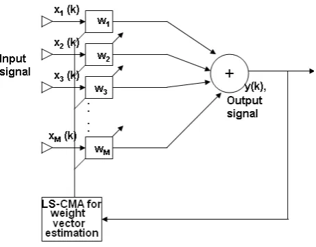
The method referred as the LSCMA algorithm [6] is also known as an autoregressive estimator based on a least squares minimization [7]. LSCMA overcomes the severe disadvantage of Godard CMA which is slow convergence time. The slow convergence creates a problem in fast varying environments in tracking the signals as well as rapidly changing channel conditions. LSCMA developed by Agee [8] is faster as compared to Godard CMA as it is based on nonlinear least square minimization. Here the cost function is weighted sum of error squares or total error energy. Figure 1 shows ABFA system using LSCMA in which the complex weights w w1, 2, ,K wMare adjusted by minimizing a certain

cost function. LSCMA compensates for the multipath signals whose constant envelope property is lost due to multipath fading, noise and interference. LSCMA has been introduced as an adaptive FIR filter for phase-modulated signals, and studied and applied to array antennas as a narrow-band adaptive beam-former to recover a constant-modulus signal [9].

In fact, the LSCMA algorithm works on the principle that the amplitude of a signal transmitted at CM and received by the array antenna should remain constant [10]. Hence, the main aim of an adaptive beam-forming based on LSCMA is to restore the average of the antenna array outputy k( ), to a

CM as illustrated in Fig. 1. Here the cost function is defined as [11]

2 1

2 2

( ) ( )

( ) K

k k

F w w

w

=

= Φ

∑

(1)

LSCMA Blind Adaptive Algorithm with Comparison of

Optimization Capabilities for Smart Antenna Systems

A. Udawat, P.C. Sharma, and S. Katiyal

Index Terms—Angle of arrival, Array Factor, LSCMA, Multipath, Smart Antenna Systems.

(2)

Fig. 1. Adaptive Beam-forming System using LSCMA

where ΦK( )w = error at th

k data sample.

( )

[

1

( ),

2

( ),

,

( )

]

T K

w

Φ

= Φ

Φ

KK

Φ

₍₂₎

K=number of data samples in one block

Equation (1) has a partial Taylor series expansion with sum-of-squares form

2 2

( ) ( ) H( ) (3)

F w+ Δ ≈ Φ w +D wΔ

where Δis an offset vector that updates weights and the complex Jacobian is defined

[

1 2

]

( ) ( ( )), ( ( )), , ( K( )) (4)

D w = ∇ Φ w ∇ Φ w _KK ∇ Φ w

One can find the offset Δwhich minimizes the sum of squared errors. Taking the gradient of “(3)” with respect to Δis given by

{

} {

}

{

}

{

}

*

* 2

2

*

( )

( ( )) 2

( ) ( ) ( ) ( )

2

( ) ( ) ( ) ( ) ( ) ( ) ( )

2

2 ( ) ( ) ( ) ( ) (5) H

H H

H

H H H H H

H F w F w

w D w w D w

w w D w w D w D w D w

w D w D w D w

Δ ∂ + Δ

∇ + Δ =

∂Δ

∂ Φ + Δ Φ + Δ

=

∂Δ

∂ Φ + Φ Δ + Δ Φ + Δ Δ

=

∂Δ

= Φ + Δ

Equating the gradient to zero one can find the optimum offset vector which minimizes (F w+ Δ)to be defined as

1

[ ( ) H( )] ( ) ( ) (6)

D w D w − w D w

Δ = − Φ

The weight vector can be updated as

1

( 1) ( ) [ ( ( )) H( ( ))] ( ( )) ( ( ))

w m+ =w m − D w m D w m −Φ w m D w m

(7) where m denotes the iteration number. The new updated

weight vector is the previous weight vector updated byΔ. The

LSCMA is derived by applying “(7)” to the CM cost function [12]

2 1

( ) ( ) 1

( ) 1 (8)

K

k

K H

k

F w y k

w x k

=

= −

∑

where ( ) H ( )

y k =w x k is array output at time k. Comparing

“(8)” with “(1)”

( ) ( ) 1

( ) 1 (9)

k

H

w y k

w x k

Φ = −

= −

Putting “(9)” into “(2)”, one can obtain (1) 1

(2) 1

( ) . (10) .

( ) 1

y

k

y K

⎡ ₋ ⎤ ⎢ ⎥

−

⎢ ⎥ ⎢ ⎥

Φ =_⎢ _⎥

⎢ ⎥ ⎢ ⎥

−

⎢ ⎥ ⎣ ⎦

The gradient vector of Φ_K( )w is given by

* *

( )

( ( )) 2

( )

( ) (11)

( ) k k

w w

w y k x k

y k ∂Φ

∇ Φ =

∂ =

Putting “(11)” into “(4)” D w( ) can be expressed as

[

1 2

]

* * *

( ) ( ( )), ( ( )), , ( ( ))

(1) (2) ( )

(1) , (2) , , ( )

(1) (2) ( )

(12)

K

CM

D w w w w

y y y K

x x x K

y y y K

XY

= ∇ Φ ∇ Φ ∇ Φ

⎡ ⎤

=⎢ ⎥

⎢ ⎥

⎣ ⎦

=

KK

where

[

(1), (2), , ( ) (13)

]

X = x x _KK x K

and

*

(1)

0 0

(1) (2)

0

(2) (14)

0

( )

0 0

( ) CM

y y

y y Y

y K y K

⎡ ⎤

⎢ ⎥

=⎢ ⎥

⎢ ⎥

⎣ ⎦

L

M

M O

L

Using “(12)” and “(10)” we can write

(15)

H H H

CM CM

H

D w D w XY Y X

XX

= =

(3)

* *

*

(1) (1)

(1) (1) 1

(2) (2) (2) 1

(2) ( ) ( )

( ) 1

( ) ( )

CM

y y

y y y

y

D w w XY X

y K

y K y K

y K

X y r

⎡ ⎤

−

⎢ ⎥

⎡ ₋ ⎤

⎢ ⎥

⎢ ₋ ⎥

−

⎢ ⎥

Φ = _⎢ _⎥= ⎢ ⎥

⎢ ⎥

⎢ ₋ ⎥

⎣ ⎦ _⎢ _⎥

−

⎢ ⎥

⎣ ⎦

= −

M

(16) where

[ (1), (2), , ( )] (17)T

y= y y KK y K

(1)_, (2)_, ( ) _{( ) (18)}

(1) (2) ( )

T

y y y K

r L L y

y y y K

⎡ ⎤

=⎢ ⎥ =

⎢ ⎥

⎣ ⎦

where ( )L y is hard limiter acting on y. Vector yand r are termed as output data vectors and complex-limited output data vector [6, 11]. Putting “(15)” and “(16)” into “(7)” one can obtain

1 *

1 1 *

1 *

( 1) ( ) [ ] ( ( ) ( ))

[ ] ( ) (19)

H

H H H

H

w m w m XX X y m r m

w m XX XX w m XX Xr m

XX Xr m

−

− −

−

+ = − −

− +

=

where

*_{( )} ( ) (1)_, ( ) (2)_, ( ) ( ) ₍₂₀₎

( ) (1) ( ) (2) ( ) ( )

T

H H H

w m x w m x w m x K

r m L

w m x w m x w m x K

⎡ ⎤

⎢ ⎥

=

⎢ ⎥

⎣ ⎦

Thus the algorithm iterates through m values until

convergence. The initial weights (1)w _{are to be chosen. The}

complex-limited output data vector *₍₁₎

r is calculated and

then w(2) is calculated. This iteration continues until satisfactory convergence is achieved.

Simulation of LSCMA adaptive algorithm for antenna arrays using 5, 8 and 10 elements separated by 0.125λ,

0.25λand 0.5λ is performed in MATLAB 7.0. The channel is assumed to be frequency selective. Here it is assumed that the CM signal is arriving at the receiver via a direct path at 45°. The direct path is assumed to be a 32 bit sequence with chip values ±1 and sampling period 4 times per chip. The block length K is assumed to be 132. The multipath signal is

arriving at -30° and is 30% of direct path signal amplitude. Due to the effect of multipath the delays in the binary sequence causes dispersion implemented by zero padding. The direct path is zero padded by adding four zeros at the back of the signal. The multipath signal is zero padded by adding two zeros at the front and two at the end. The zero mean Gaussian noise for each antenna element is added and the noise variance is 0.01. The initial weights are assumed to be 1. Following cases are considered.

A. Case 1

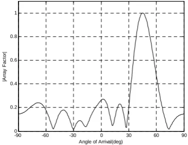
Figure 2, 3 and 4 shows the array factor plots for LSCMA with number of elements N=5, 8 and 10 for 06 iterations for

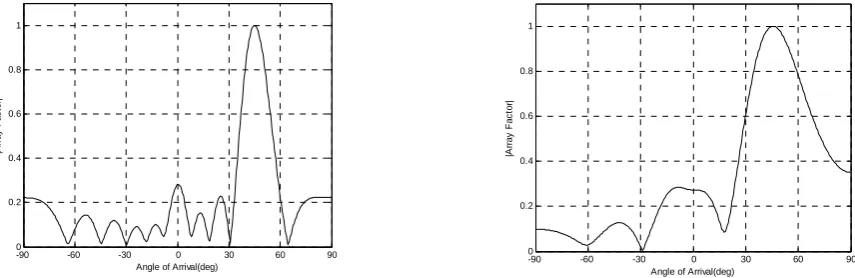
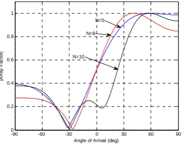
inter-element separation d=0.5λ respectively. From fig. 5 (combined plot of fig. 2, 3 and 4) it is clear that LSCMA generates peak in the desired direction user AOA 45º and places nulls in the undesired direction where interferer is located i.e., at -30º. Figure 5 shows that the number of side-lobes (SL) increases with N with a decrease in

beam-width and increase in gain. The most optimized value for N is 8 with better gain and less number of SL levels

(SLL). Figure 5 shows that the gain improves to 47.75 dB (N= 10) from 42.09 dB (N= 8), 33.22 dB (N= 5), the level

of SL degrades to 0.1 (N= 10) from 0.2 (N= 8), 0.3 (N= 5)

and the beam-width decreases to 13° (N= 10) from 18° (N=

8), 30° (N= 5). Also the number of SL increases to 7 (N=

10) from 6 (N= 8), 4 (N= 5). In terms of generating nulls in

the direction of interferers, appreciable reduction in levels at -30° is observed.

B. Case 2

The variation of array factor for LSCMA with number of elements equal to N= 5, 8 and 10 for 06 iterations are drawn

for different inter-element separation d=0.25λ (figure 6, 7 and 8) and d=0.125λ (figure 10, 11 and 12). Figure 9 (combined plot of Figure 6, 7 and 8) and 13 (combined plot of Figure 10, 11 and 12) shows that performance of LSCMA degrades as indicated by an increase in beam-width. More levels at interferer AOA -30° are observed. Thus inter-element spacing must be 0.5λas can be concluded from

Case 1 and 2.

-90 -60 -30 0 30 60 90

0 0.2 0.4 0.6 0.8 1

Angle of Arrival(deg)

|A

rray

F

a

c

to

r|

Fig. 2. Array factor plot for LSCMA with user AOA 45° and interferer AOA at -30° for N = 5 and d=0.5λ

-90 -60 -30 0 30 60 90

0 0.2 0.4 0.6 0.8 1

|A

rr

ay

F

a

c

tor|

(4)

-90 -60 -30 0 30 60 90 0

0.2 0.4 0.6 0.8 1

|A

rr

a

y

F

a

c

to

r|

Fig. 4. Array factor plot for LSCMA with user AOA 45° and interferer AOA at -30° for N = 10 and d=0.5λ

-90 -60 -30 0 30 60 90

0 0.2 0.4 0.6 0.8 1

Angle of Arrival (deg)

|A

rra

y

F

a

c

tor|

N=5

N=8

N=10

Fig. 5. Array factor plot for LSCMA with user AOA 45° and interferer AOA at -30° for N = 5, 8, 10 and d=0.5λ

-90 -60 -30 0 30 60 90

0 0.2 0.4 0.6 0.8 1

|A

rr

a

y

F

a

c

to

r|

-90 -60 -30 0 30 60 90

0 0.2 0.4 0.6 0.8 1

|A

rr

ay

F

a

c

tor

|

-90 -60 -30 0 30 60 90

0 0.2 0.4 0.6 0.8 1

|A

rra

y

F

a

c

to

r|

-90 -60 -30 0 30 60 90

0 0.2 0.4 0.6 0.8 1

|A

rr

a

y

F

a

c

to

r|

N=5

N=8

N=10

-90 -60 -30 0 30 60 90

0 0.2 0.4 0.6 0.8 1

|A

rr

a

y

F

a

c

to

r|

-90 -60 -30 0 30 60 90

0 0.2 0.4 0.6 0.8 1

|A

rr

ay

F

ac

tor

|

(5)

-90 -60 -30 0 30 60 90 0

0.2 0.4 0.6 0.8 1

|A

rr

a

y F

a

cto

r|

-90 -60 -30 0 30 60 90

0 0.2 0.4 0.6 0.8 1

|A

rr

a

y F

a

cto

r|

N=5

N=8

N=10

IV. CONCLUSION

In this paper the optimization capabilities of LSCMA blind adaptive beam-forming algorithm are explored and it is found that for inter-element spacing of 0.5λ with 8 elements the beam-width of 18° is achieved with a gain of 42.09dB. The number of iterations required is 03. LSCMA does not require ( )d k the reference signal and thus bandwidth can be

saved. Thus the most optimum values obtained for antenna array using LSCMA are N =8 (no. of elements) and

0.5

d= λ (inter-element spacing).

REFERENCES

[1] S. F. Shaukat, M. Hassan, R. Farooq, H. U. Saeed and Z. Saleem, “Sequential Studies of BFA for SAS”, World Applied Science Journal 6, pp 754-758, 2009.

[2] S. Rani, P. V. Subbaiah and K. C. Reddy, “LMS and RLS Algorithm for Smart Antennas in a WCDMA Mobile Communication

Environment”, ARPN Journal of Engineering and Applied Sciences,

Vol.4 No.6, pp. 78-88, August 2009.

[3] D. N. Godard, “Self-recovering equalization and carrier tracking in two-dimensional data communication systems,” IEEE Trans. Comm., vol. 28, no. 11, pp. 1867–1875, Nov. 1980.

[4] J. R. Treichler and B. G. Agee, “A new approach to multipath correction of constant modulus signals,” IEEE Trans. Acoust., Speech, Signal Processing, vol. 31, no. 2, pp. 459–472, Apr. 1983.

[5] Guo Yecai, Yang Chao, “Frequency Domain Constant Modulus Algorithm Based on Fractionally Spaced Blind Equalizer”,

Proceedings of the 2009 International Workshop on Information Security and Application (IWISA 2009) Qingdao, China, November 21-22, 2009.

[6] Rong, Z., “Simulation of Adaptive Array Algorithms for CDMA Systems,” Master’s Thesis MPRG-TR-96-31, Mobile & Portable Radio Research Group, Virginia Tech, Blacksburg, VA, Sept. 1996.

[7] Stoica, P., and R. Moses, Introduction to Spectral Analysis, Prentice

Hall, New York, 1997.

[8] Salma Ait Fares and Fumiyuki Adachi, “Mobile and Wireless Communications: Physical layer development and implementation”,

In-The Olajnica, Vukovar, Croatia, 2010.

[9] L.C. Godara, "Applications of Antenna Arrays to Mobile Communications. I. Performance Improvement, Feasibility, and System Considerations," Proceedings of IEEE, Volume 85, Issue 7,

July 1997, Pages 1031-1060

[10] S. W. Varade and K. D. Kulat, “Robust Algorithms for DoA Estimation and Adaptive Beamforming for Smart Antenna Application”, 2nd

International Conference on Emerging Trends in Engineering and Technology, ICETET-09.

[11] Frank Gross, “Smart Antenna For Wireless Communication”

Mcgraw-Hill, September 14, 2005.

[12] Lal C. Godara, “Application of Antenna Arrays to Mobile Communications, Part П: Beam-forming and Direction-of-Arrival considerations”, Proceeding of the IEEE, Vol. 85, No. 8, pp. 1195- 1234, August 1997.

A. Udawat was born in Indore (M.P.), India on 27th

June 1977. He received B.E. in Electronics and Communication Engineering from Shri Vaishnav Institute of Technology and Science, DAVV, Indore, India in 2000 and M.E. in Electronics and Communication from SGSITS, RGPV, Indore, India in 2007.

He joined Electronics and Communication Department as Lecturer in Medi-Caps Institute of Technology and Management in August 2001. He is presently working as Associate Professor in Medicaps Institute of Technology and Management, Indore, India. He is pursuing Ph. D from School of Electronics, DAVV, Indore (M.P.), India. His topic of research is Adaptability in Algorithms and Optimization for smart Antenna Systems. The format for listing publishers of a book within the biography is: “Comparison of Different Angle of Arrival Estimation Techniques with Resolution Capabilities for Smart Antenna Systems in Wireless Communication”,(Radio Engineering Journal Engineering and Technology, 2011). “Comparison of SMI and LMS Algorithm with Optimization Capabilities for Smart Antenna Systems in Multipath Environment”,(International Journal of Engineering, 2011).”CMA Blind Adaptive Algorithm with Comparison of Optimization Capabilities for Smart Antenna Systems”, (International Conference WorldComp-2011, Lasvegas, Nevada, USA)