Abstract— A comparative study of pressure distribution and load capacity of a cylindrical bore journal bearing is presented in this paper. In calculating the pressure distribution and load capacity of a journal bearing, isothermal analysis was carried out. Using both analytical method and finite element method, pressure distribution in the bearing was calculated. Moreover, the effects of variations in operating variables such as eccentricity ratio and shaft speed on the load capacity of the bearing were calculated. The analytical results and finite element results were compared. In order to check the validity, these results were also compared with the available published results. In comparison with the published results, generally finite element results showed better agreement than analytical results.
Index Term— Analytical Method, Finite Element Method, Journal Bearing, Load Capacity, Pressure Distribution.
I. INTRODUCTION
Wear is the major cause of material wastage and loss of mechanical performance of machine elements, and any reduction in wear can result in considerable savings which can be made by improved friction control. Lubrication is an effective means of controlling wear and reducing friction, and it has wide applications in the operation of machine elements such as bearings. The principles of hydrodynamic lubrication were first established by a well known scientist Osborne Reynolds and he explained the mechanism of hydrodynamic lubrication through the generation of a viscous liquid film between the moving surfaces. The journal bearing design parameter such as load capacity can be determined from Reynolds equation both analytically and numerically.
Numerical analysis has allowed models of hydrodynamic lubrication to include closer approximations to the characteristics of real bearings. Numerical solutions to hydrodynamic lubrication problems can now satisfy most engineering requirements for prediction of bearing characteristics. To analyze the bearing design parameters, several approximate numerical methods have evolved over the years such as the finite difference method and the finite
element method. The finite difference method is difficult to use when irregular geometries are to be solved. Nowadays finite element method becomes more popular and can overcome these difficulties. Use of elements and interpolation functions ensure continuity of pressure and mass flow rate across inter-element boundaries. Booker and Huebner used finite element method for the solution of hydrodynamic lubrication problems [1]. Later Hayashi and Taylor used the finite element technique to predict the characteristics of a finite width journal bearing [2]. A theoretical investigation was carried out by Gethin and Medwell using the finite element method for a high speed bearing [3]. A theoretical study based on the finite element method was carried out by Gethin and Deihi to investigate the performance of a twin-axial groove cylindrical bore bearing [4]. Basri and Gethin worked on the finite element method for the solution of hydrodynamic lubrication problems [5]. A theoretical and experimental study of thermal effects in a plain circular steadily loaded journal bearing was carried out by Ma and Taylor [6]. In comparing the global performance characteristics, theory and experiment exhibited an excellent agreement over a wide range of loads and rotational speeds. Gethin worked on the thermal behavior of various types of high speed journal bearings and found good agreement with theoretical and the experimental results [7].
The effects of variable density and variable specific heat on maximum pressure, maximum temperature, bearing load, frictional loss and side leakage in high-speed journal bearing operation were examined [8]. The combined effects of couple stress due to a Newtonian lubricant blended with additives and the presence of roughness on journal bearing surfaces were examined [9]. It was found that the couple stress effects can raise the film pressure of the lubricant fluid, improve the load-carrying capacity and reduce the friction parameter, especially at high eccentricity ratio. The surface roughness effect is dominant in long bearing approximation and the influence of transverse or longitudinal roughness to the journal bearing is in reverse trend. Hydrodynamic lubrication characteristics of a journal bearing, taking into consideration the misalignment caused by shaft deformation were analyzed [10]. Film pressure, load-carrying capacity attitude angle, end leakage
Study on Pressure Distribution and Load
Capacity of a Journal Bearing Using Finite
Element Method and Analytical Method
D. M. Nuruzzaman
, M. K. Khalil, M. A. Chowdhury, M. L. Rahaman
Department of Mechanical Engineering
Dhaka University of Engineering & Technology, Gazipur, Gazipur - 1700, Bangladesh
103605-7474 IJMME-IJENS © October 2010 IJENS I J E N S flow rate, frictional coefficient and misalignment moment were
calculated for different values of misalignment degree and eccentricity ratio. It was found that there are obvious changes in film pressure distribution, the highest film pressure, film thickness distribution, the least film thickness and the misalignment moment when misalignment takes place. The distributions of pressure, temperature and oil flow velocity of a journal bearing with a two-component surface layer were investigated [11]. It was found that a journal with a two-component surface layer causes a reduction in the bearing load capacity for high eccentricity ratio. Besides, considerable velocity changes in oil flow in all directions (circumferential, radial and axial) were observed particularly, great velocity changes occurred in the radial direction. Effects of test conditions on the tribological behavior of a journal bearing in molten zinc were investigated [12]. It was found that the bearings appear to have a smoother running condition at higher rotation speeds and when tested at the same load, reduction of the speed resulted in higher friction and more wear of the bearings. Thermohydrodynamic analysis of herringbone grooved journal bearings (HGJB) showed that the temperature of the fluid film rises significantly due to the frictional heat, thereby the viscosity of the fluid and the load carrying capacity decreases [13]. It is found that HGJB has a better load carrying capacity and low end leakage as compared to plain journal bearing. It is also observed that the HGJB is more stable than the conventional plain journal bearing. Temperature profile of an elliptic bore journal bearing was investigated [14]. It was found that with increasing non-circularity the pressure gets reduced and the temperature rise is less in the case of a journal bearing with higher non-circularity value. A comparative study for rise in oil-temperatures, thermal pressures and load carrying capacity has been carried out for the analysis of
elliptical journal bearings [15] and in this
thermohydrodynamic analysis finite difference method has been adopted for numerical solution of the Reynolds and energy equation. It was found that oil film temperature and thermal pressures in the central plane of the elliptical bearing increase with the increase in the speed and eccentricity ratio.
Currently, there is very little information about the comparison between the finite element results and the analytical results to discuss the pressure distribution and load capacity of a cylindrical bore journal bearing. So, to understand this issue more clearly, this paper presents a comparison between the finite element results and the analytical results of pressure distribution and load capacity of a cylindrical bore journal bearing. Moreover, these obtained results are compared with the available published data.
II. THEORETICALBACKGROUND AND CALCULATION
PROCEDURE
A.Assumptions
i) Newtonian fluid is considered ii) Thermal effects are neglected iii) Fluid density is constant iv) No slip at the boundaries
B.Finite Element Method
The finite element method (FEM) has been used for the numerical modeling of a cylindrical bore journal bearing to calculate the pressure distribution and load capacity. In this analysis, to discretize the governing Reynolds equation, Galerkin weighted residual approach has been adopted. In the numerical model, a finite element mesh was considered. The load bearing film was divided into a finite number of eight-node isoparametric elements of serendipity family. The overall solution procedure was completed by iteration and pressure field had converged, and finally the usual bearing design parameter the load capacity was calculated. These results were compared with the analytical results. These results were also compared with the available published results.
Formulation of Governing Equation:
The governing Reynolds differential equation is:
x
h
p
x
y
h
p
y
U dh
dx
(
)
(
)
3
12
3
12
2
(1)Now for Reynolds equation:
0
2
12
3
12
3
d
i
dx
dh
U
y
p
h
y
x
p
h
x
where
i is the shape function.
Writing these equations in general matrix form:
8
.
.
2
1
8
.
.
2
1
88
...
82
81
.
.
.
.
.
.
28
...
22
21
18
...
12
11
F
F
F
a
a
a
K
K
K
K
K
K
K
K
K
(2) where Ki j and Fi are the stiffness and load term respectively.
Each shape function is a Lagrange quadratic polynomial which satisfies the interpolation property
)
,
(
22
)
,
(
21
)
,
(
12
)
,
(
11
)
,
(
J
J
J
J
y
x
y
x
J
The determinant of the Jacobian matrix
J
( , )
is called the Jacobian.So the stiffness and load integral terms are:
Ki j
x
J
d
d
j
x
i
h
)
,
(
1
1
1
1 12
3
y
J
d
d
j
y
i
h
)
,
(
1
1
1
1 12
3
(4)
J
d
d
dx
dh
U
i
F
(
,
)
2
1
1
1
1
(5)
Using equations (4) and (5), equation (2) is solved for load capacity of the bearing.
C.Analytical Method
In the analytical method, the load carrying film was divided into a mesh of four-node rectangular elements. The coordinate value of each node was calculated and the film thickness at each nodal point was determined. The film pressure was solved at various nodal points. The film geometry was updated, the new coordinates were determined and the new film thickness was calculated until the pressure field was optimized. Finally the usual bearing design parameter such as load capacity was calculated for a range of eccentricity ratio and shaft speed. These results were compared with the finite element results. These results were also compared with the available published results.
Formulation of Governing Equation:
For a narrow bearing, the pressure gradient along the axial direction is much larger than the pressure gradient along the circumferential direction. For this narrow bearing approximation, the governing one dimensional Reynolds equation is:
p
U
h
dh
dx
y
L
3
3
2
2
4
(
)
(6)This gives the pressure distribution as a function of film
thickness gradient dh
dx where the film thickness is defined as:
h e
cos
C
C
(
1
cos
)
(7)Using equation [6], the bearing design parameter such as load capacity was calculated for a range of eccentricity ratio and shaft speed.
III. RESULTANDDISCUSSION
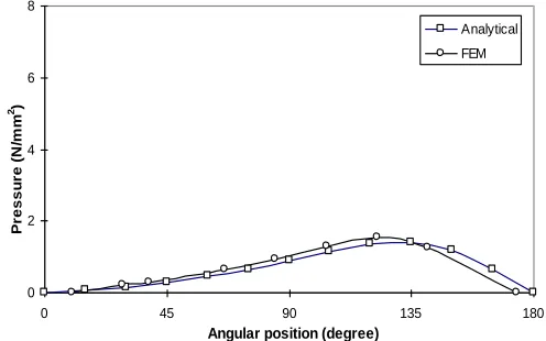
Figure 1 illustrates the circumferential pressure distribution against angular position for a fixed eccentricity ratio of 0.4 and at shaft speed N=5000 rpm, L/R = 1.0 and C/R = 0.004. From the analytical and FEM results, it was seen that pressure increased steadily from zero to the maximum value and then decreased steadily to zero. Both analytical and FEM results showed similar trends and the agreement between the FEM and analytical results was quite satisfactory. Figure 2 shows the mid plane pressure distribution with the shaft turning at 10000 rpm and eccentricity ratio=0.4, L/R = 1.0 and C/R = 0.004. The hydrodynamic pressure profile gradually increased from zero and reached the maximum and then gradually decreased to zero. The FEM results were compared with analytical results and the agreement was good. Figure 3 also illustrates the pressure distribution for eccentricity ratio = 0.5, L/R = 1.0, C/R = 0.004 and shaft speed N=5000 rpm. From the analytical and FEM results, it was seen that the pressure increased steadily from zero and reached the maximum and then gradually decreased to zero. Descrepancy was found between analytical results and finite element results because the analytical solution used Half-Sommerfeld boundary condition but the finite element solution used Reynolds boundary condition. In Figure 4, circumferential pressure distribution with angular position is shown for shaft speed N = 10000 rpm, eccentricity ratio = 0.5, L/R = 1.0 and C/R = 0.004. From the FEM and analytical results it was seen that pressure increased gradually from zero and reached the maximum and then gradually decreased to zero. Descrepancy was found between analytical results and finite element results because the analytical solution used Half-Sommerfeld boundary condition whereas the finite element solution used Reynolds boundary condition.
Figure 26: Variation of pressure with angular position. 0
2 4 6 8
0 45 90 135 180
Angular position (degree)
Pr e s s u re (N /m m 2) Analytical FEM
103605-7474 IJMME-IJENS © October 2010 IJENS I J E N S In Figure 5, the mid plane pressure distribution at different
angular position is shown for eccentricity ratio = 0.8, L/R = 1.0, C/R = 0.004 and Re = 500. The results are shown in dimensionless form. The analytical solution used Half-Sommerfeld boundary condition and only positive pressure
region was considered. From the results, it was found that the hydrodynamic pressure profile increased steadily from zero and it changed very rapidly in the area of the smallest film thickness and reached to a maximum. In this region the film was convergent. The pressure then gradually dropped to zero. When the analytical results were compared with Gethin and Deihi’s results, about 75% accuracy was achieved. This descrepancy was found because the analytical solution used Half-Sommerfeld boundary condition but Gethin and Deihi used Reynolds boundary condition. Figure 6 illustrates the mid plane pressure distribution at different angular position for eccentricity ratio = 0.8, L/R = 1.0, C/R = 0.004 and Re = 500. The finite element results are shown in dimensionless form. The solution used Reynolds boundary condition and only positive pressure region was considered. The results showed that the hydrodynamic pressure profile increased steadily from zero and it changed very rapidly in the area of the smallest film thickness and reached to a maximum. In this region the film was convergent. The pressure then gradually dropped to zero. In order to check the validity, when these results were compared with Gethin and Deihi’s results, a strong resemblance was obtained and about 90% accuracy was achieved.
Figure 27: Variation of pressure with angular position. 0
2 4 6 8
0 45 90 135 180
Angular position (degree)
Pr
e
s
s
u
re
(N
/m
m
2)
Analytical FEM
Fig. 2. Variation of pressure with angular position (N=10000 rpm, ε=0.4)
Figure 28: Variation of pressure with angular position. 0
2 4 6 8
0 45 90 135 180
Angular position (degree)
Pr
e
s
s
u
re
(N
/m
m
2)
Analytical FEM
Fig. 3. Variation of pressure with angular position (N=5000 rpm, ε=0.5)
Figure 29: Variation of pressure with angular position. 0
2 4 6 8
0 45 90 135 180
Angular position (degree)
Pr
e
s
s
u
re
(N
/m
m
2)
Analytical FEM
Fig. 4. Variation of pressure with angular position (N=10000 rpm, ε=0.5)
Figure 12: Variation of dimensionless pressure with angular position
0 2 4 6 8 10
0 45 90 135 180
Angular position
D
im
e
n
s
io
n
le
s
s
p
r
e
s
s
u
r
e
Gethin and Deihi Analytical
Fig. 5. Variation of dimensionless pressure with angular position (Re=500, ε=0.8)
Figure 19: Variation of dimensionless pressure with angular position
0 2 4 6 8 10
0 45 90 135 180
Angular position
D
im
e
n
s
io
n
le
s
s
p
r
e
s
s
u
r
e
Gethin and Deihi FEM
Figure 7 exhibits the circumferential pressure distribution at different angular position for a fixed eccentricity ratio = 0.8, L/R=1.0, C/R = 0.004 and Re = 500. Analytical and FEM results are shown in dimensionless form. Only positive pressure region was considered. The hydrodynamic pressure profile increased steadily from zero and it changed very rapidly in the area of the smallest film thickness and reached to a maximum. In this region the film was convergent. The pressure then gradually dropped to zero. When analytical and FEM results were compared with Gethin and Deihi’s results, it was apparent that FEM results showed better agreement than analytical results. Figure 8 shows the circumferential pressure distribution with angular position for R = 40 mm, eccentricity ratio = 0.87, L/R = 1.27, C/R = 0.008 and shaft speed N = 1000 rpm. Only positive pressure region was considered. The hydrodynamic pressure increased very steadily from zero and it changed very rapidly in the area of smallest film thickness
and reached to a maximum. In this region the film was convergent. The pressure then gradually dropped to zero. The graphs for analytical and FEM results showed similar trends of variation and when these results were compared with those
obtained experimentally by Gethin and Medwell, it was quite clear that although the shape of the experimental pressure distribution followed that predicted by hydrodynamic theory, the magnitudes of the pressures were much less than those predicted. Peak pressure by experiment was less than those predicted by approximately 30%. During the experiment, the bearing continued to run in thermal conditions and thermal gradients in the lubricant film are responsible for the discrepancies between the experimental data and those predicted from the hydrodynamic model that assumes an isothermal film.
The variation of load capacity with eccentricity ratio is illustrated in Figure 9 for L/R = 1.0, C/R = 0.004 and speed N = 10000 rpm. From the FEM and analytical results, it was seen that the load capacity of the bearing increased gradually with eccentricity ratio. A comparison between the FEM and analytical results showed that the agreement was satisfactory. Figure 10 also illustrates the variation of load capacity with shaft speed ranging from 5000 rpm to 20000 rpm. In this case, eccentricity ratio = 0.6, L/R = 1.0 and C/R = 0.004. The results indicated that the load capacity increased with the increase of shaft speed. Further comparison of FEM results with analytical results showed similar trends of variation and a good agreement was achieved.
Figure 42 :Variation of dimensionless pressure with angular position 0
2 4 6 8 10
0 45 90 135 180
Angular position
D
im
e
n
s
io
n
le
s
s
p
re
s
s
u
re
Gethin and Deihi FEM Analytical
Fig. 7. Variation of dimensionless pressure with angular position (Re=500, ε=0.8)
Fig. 8. Circumferential pressure distribution with angular position (N=1000 rpm, ε=0.87)
Figure 49 :Circumferential pressure distribution with angular position
0 1 2 3
0 50 100 150 200
Angular position
P
r
e
s
s
u
r
e
(
N
/s
q
.m
m
)
Exp.(Gethin and Medwell) FEM
Analytical
Figure 31: Variation of load capacity with eccentricity ratio
0 20 40 60
0.3 0.4 0.5 0.6 0.7 0.8 0.9
Eccentricity ratio
L
o
a
d
c
a
p
a
c
ity
(k
N
)
Analytical
FEM
Fig. 9. Variation of load capacity with eccentricity ratio (N=10000 rpm)
0 20 40 60
5000 8000 11000 14000 17000 20000
rpm
L
o
a
d
c
a
p
a
c
ity
(k
N
)
Analytical
FEM
103605-7474 IJMME-IJENS © October 2010 IJENS I J E N S A systematic series of calculations was computed for the
dimensionless load variation at different eccentricity ratio for R = 50 mm, C/R = 0.004, L/R = 1.0 and Re = 1000. The analytical results are shown in Figure 11. From the graph it is clear that at low eccentricity ratio, the dimensionless load increases gradually but it is greatly increased with high eccentricity ratio. In comparison with the results obtained by Gethin and Deihi, the analytical results showed similar trends and about 80% accuracy was achieved. Figure 12 illustrates the variation of load capacity with shaft speed ranging from 5000 rpm to 20000 rpm for R = 50 mm, L/R = 1.0, C/R = 0.004 and eccentricity ratio = 0.7. It was apparent from analytical results that load capacity increased gradually with the increase of shaft speed. When these results were compared with those presented by Gethin and Medwell, 65% accuracy was obtained.
Figure 13 illustrates the dimensionless load variation at different eccentricity ratio for R = 50 mm, C/R = 0.004, L/R = 1.0 and Re = 1000. From the finite element results it was apparent that at low eccentricity ratio, the dimensionless load increased gradually but it was greatly increased with high eccentricity ratio. The comparison of these results with Gethin
and Deihi’s results showed very good agreement and about 90% accuracy was achieved. Figure 14 shows the variation of
load capacity with the shaft speed ranging from 5000 rpm to 20000 rpm for R = 50 mm, L/R = 1.0, C/R = 0.004 and eccentricity ratio = 0.7. From the finite element results it was clear that the load capacity increased gradually with the increase of shaft speed. The comparison of these results with those presented by Gethin and Medwell showed good agreement and about 80% accuracy was obtained.
Figure 15 shows that a systematic series of calculations was computed for the dimensionless load variation at different eccentricity ratio for R = 50 mm, C/R = 0.004, L/R = 1.0 and Re = 1000. From FEM and analytical results, it was seen that at low eccentricity ratio the dimensionless load increased steadily and it was greatly increased with high eccentricity ratio. The results from FEM and analytical method were compared with the results obtained by Gethin and Deihi, a strong resemblance was achieved. Moreover, it was quite clear that in comparison with the published results, FEM results showed better agreement than analytical results. Figure 16 illustrates the variation of load capacity with shaft speed ranging from 5000 rpm to 20000 rpm for R = 50 mm, L/R = 1.0, C/R = 0.004 and eccentricity ratio = 0.7. It was apparent Figure 13: Variation of dimensionless load with eccentricity
ratio. 0
20 40 60
0.3 0.4 0.5 0.6 0.7 0.8 0.9
Eccentricity ratio
D
im
e
n
s
io
n
le
s
s
l
o
a
d
Gethin and Deihi
Analytical
Fig. 11. Variation of dimensionless load with eccentricity ratio (Re=1000)
Figure 14: Variation of load capacity with rpm 0
20 40 60
5000 8000 11000 14000 17000 20000
rpm
L
o
a
d
c
a
p
a
c
ity
(k
N
)
Gethin and Medw ell Analytical
Fig. 12. Variation of load capacity with shaft speed (ε=0.7)
Figure 20: Variation of dimensionless load with eccentricity ratio.
0 20 40 60
0.3 0.4 0.5 0.6 0.7 0.8 0.9
Eccentricity ratio
D
im
e
n
s
io
n
le
s
s
l
o
a
d
Gethin and Deihi
FEM
Fig. 13. Variation of dimensionless load with eccentricity ratio (Re=1000)
Figure 21: Variation of load capacity with rpm
0 20 40 60
5000 8000 11000 14000 17000 20000
rpm
L
o
a
d
c
a
p
a
c
ity
(k
N
)
Gethin and Medw ell FEM
from the FEM and analytical results that load capacity increased with the increase of shaft speed. When these results were compared with those presented by Gethin and Medwell, it revealed that FEM results showed better performance than analytical results.
Figure 17 illustrates the variation of load capacity with eccentricity ratio for R = 36.7 mm, L/R = 1.0, C/R = 0.002 and N = 20000 rpm. Analytical and FEM results showed similar trends of variation and at low eccentricity ratio load capacity was low but at high eccentricity ratio it increased remarkably. These results were compared with those obtained
experimentally by Gethin and Medwell and from the graphs it is apparent that at very high surface speed, the agreement deteriorates as the eccentricity ratio increases. At eccentricity ratio 0.8, load capacity by experiment was approximately 45% less than those predicted. At high surface speed thermal gradients set up in the lubricant film are responsible for the discrepancies between the experimental results and those obtained by the isothermal hydrodynamic theory. Figure 18 also shows the variation of load capacity with shaft speed ranging from 20000 rpm to 26000 rpm. From the graphs it is seen that analytical and FEM results show similar trends and load capacity increases with the increase of shaft speed. In comparison with the experimental results, it is very clear that beyond the speed 22000 rpm, load capacity by experiment decreased with the increased shaft speed and at speed 26000 rpm, load capacity by experiment was approximately 50% of those predicted. This is due to the severe deterioration of the lubricant viscosity with increased frictional heat generation at higher surface speed.
IV. CONCLUSION
Pressure distribution and load capacity of a cylindrical bore journal bearing were calculated using finite element method and analytical method. In the calculation, isothermal analysis and Newtonian fluid film behavior were considered. In the numerical method, a finite element mesh was considered and Galerkin weighted residual approach has been adopted. In the analytical method, the load carrying film was divided into a mesh of four-node rectangular elements. For fixed shaft speed and eccentricity ratio, fluid film pressures at different circumferential positions of the bearing were calculated. When the finite element results and analytical results were compared, in general, the agreement was found quite satisfactory. Moreover, the effects of variation in eccentricity ratio and shaft speed on the load capacity of the bearing were calculated. The finite element results and analytical results were compared and the agreement was found satisfactory. When these results were compared with available published results, good resemblance was achieved which confirms the Figure 43: Variation of dimensionless load with eccentricity
ratio. 0
20 40 60
0.3 0.4 0.5 0.6 0.7 0.8 0.9
Eccentricity ratio
D
im
e
n
s
io
n
le
s
s
l
o
a
d
Gethin and Deihi FEM
Analytical
Fig. 15. Variation of dimensionless load with eccentricity ratio (Re=1000)
Figure 44: Variation of load capacity with rpm 0
20 40 60
5000 8000 11000 14000 17000 20000
rpm
L
o
a
d
c
a
p
a
c
ity
(k
N
)
Gethin and Medw ell FEM
Analytical
Fig. 16. Variation of load capacity with shaft speed (ε=0.7)
Figure 50: Variation of load capacity with eccentricity ratio.
0 2 4 6 8
0.5 0.6 0.7 0.8
Eccentricity ratio
L
o
a
d
c
a
p
a
c
ity
(k
N
)
Exp.(Gethin and Medw ell) FEM
Analytical
Fig. 17. Variation of load capacity with eccentricity ratio (N=20000 rpm)
Figure 51: Variation of load capacity with rpm 0
2 4 6 8
20000 22000 24000 26000
rpm
L
o
a
d
c
a
p
a
c
ity
(k
N
)
Exp.(Gethin and Medw ell)
FEM
Analytical
103605-7474 IJMME-IJENS © October 2010 IJENS I J E N S numerical model. As a whole, with comparison to available
published results, finite element results showed better agreement than analytical results.
NOTATION
p
Film pressureh
Film thickness U Surface speed of shaft Re Reynolds number L Bearing axial length R Journal radius C Radial clearance N Shaft speed e Eccentricity Eccentricity ratio
Angular position of shaft
Domain of calculation
j Shape functionK
i j Stiffness matrix term ati j
,
F
i Load matrix termJ( , ) Jacobian matrix
Lubricant viscosityREFERENCES
[1] J.F. Booker and K.H. Huebner, “Application of Finite Elements to Lubrication: An Engineerimg Approach,” Journal of Lubrication Technology, Trans. ASME, vol.24, no. 4, pp. 313-323, 1972.
[2] H. Hayashi and C.M. Taylor, “A Determination of Cavitation Interfaces in Fluid Film Bearings Using Finite Element Analysis,” Journal Mechanical Engineering Science, vol. 22, no. 6, pp.277-285, 1980. [3] D.T. Gethin and J.O. Medwell, “An Investigation into the Performance
of a High Speed Journal Bearing with two Axial Lubricant Feed Grooves,”Project Report, University of Wales, 1984.
[4] D.T. Gethin and M.K.I. EI Deihi, “Effect of Loading Direction on the Performance of a Twin Axial Groove Cylindrical Bore Bearing”, Tribology International, vol. 20, no. 3, pp. 179-185, 1987.
[5] S. Basri and D.T. Gethin, “A Comparative Study of the Thermal Behaviour of Profile Bore Bearings,” Tribology International, vol. 4, no. 12, pp. 265-276, 1990.
[6] M.T. Ma and C.M. Taylor, “A Theoretical and Experimental Study of Thermal Effects in a Plain Circular Steadily Loaded Journal Bearing,” Transactions IMechE, vol. 824, no. 9, pp. 31-44, 1992.
[7] D.T. Gethin, “Thermohydrodynamic Behaviour of High Speed Journal Bearings,” Tribology International, vol. 29, no. 7, pp. 579-596, 1996. [8] S.M. Chun, “Thermohydrodynamic lubrication analysis of high-speed
journal bearing considering variable density and variable specific heat,” Tribology International, vol. 37, pp. 405-413, 2004.
[9] H.L. Chiang, C.H. Hsu, J.R. Lin, “Lubrication performance of finite journal bearings considering effects of couple stresses and surface roughness,” Tribology International. vol. 37, pp. 297-307, 2004. [10] J. Sun, G. Changlin, “Hydrodynamic lubrication analysis of journal
bearing considering misalignment caused by shaft deformation,” Tribology International, vol. 37, pp. 841-848, 2004.
[11] J. Sep, “Three dimensional hydrodynamic analysis of a journal bearing with a two component surface layer,” Tribology International, vol. 38, pp. 97-104, 2005.
[12] K. Zhang, “Effects of test conditions on the tribological behavior of a journal bearing in molten zinc,” Wear, vol. 259, pp. 1248-1253, 2005. [13] M. Sahu, M. Sarangi, B.C. Majumdar, “Thermohydrodynamic analysis
of herringbone grooved journal bearings,” Tribology International, vol. 39, pp. 1395-1404, 2006.
[14] P.C. Mishra, R.K Pandey, K. Athre, “Temperature profile of an elliptic bore journal bearing,” Tribology International, vol. 40, pp. 453-458, 2007.