Plane Stabilization of the Electron Storage Ring Using Automatic 3-DOF Girder System

(1)

Abstract— The plane stabilization of 1.2 GeV electron storage

ring of the Siam Photon Source has changed one millimeter per year resulted from the occurrences of floor subsidence. The alignment takes approximately three months which requires a lot of manpower. This paper presents the new technique of the control system design and mathematical model of the automatic 3-DOF girder system for aligning the magnets in the electron storage ring. The girder system is designed based on three eccentric circle cam actuators with DC motor which are translation along the y-axis (heave), rotation around the x-axis (pitch) and the z-axis (roll). The control system consists of two control loops: a) the inner control loop which is composed of three actuators used the angular position control with pole-placement through the state feedback with full-order state observer and b) the outer control loop which tracks control of the girder system with proportional-integral controller tuning using the optimization method based on the simplex search method. The performance of the automatic 3-DOF girder system is supported by simulation and experimental results. Therefore, the experimental results show that it exactly and quickly tracks the reference input and robustly regulates the output response which has the external disturbances. This prototype is appropriate for the development of the magnet girder system for the electron storage ring.

Index Term— angular position control, observer-based state

feedback controller, tracking control and output regulation, PI-controller, 3-DOF girder system, eccentric circle cam actuator

I. INTRODUCTION

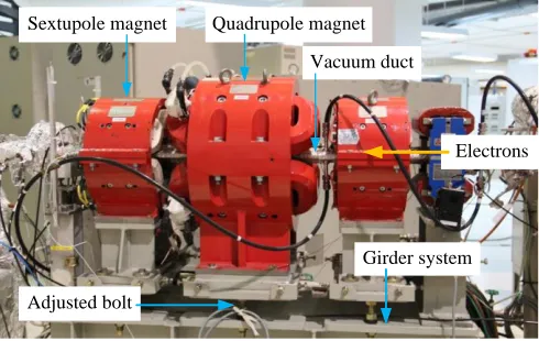
The 1.2 GeV electron storage ring of the Siam Photon Source (SPS) at the Synchrotron Light Research Institute (SLRI) has produced the synchrotron light using the magnetic field to change the electron directions, emit light, and store the electrons. The synchrotron light is provided to scientists for their various research [1]-[3]. The occurrences of floor subsidence cause the plane stabilization of the electron storage ring with a circumference is 81.3 meters have been changing by one millimeter per year. The magnet girder system of the SPS electron storage ring is shown in Fig. 1. The alignment process of all magnets in the electron storage ring takes approximately three months and requires a lot of manpower [4], [5]. Consequently, the solution to this problem is to apply the automatic girder system in which the alignment is precisely and quickly with less manpower [6], [7]. Their use of iterative techniques for the control of the girder system. This paper presents the new technique of the control system design, the mathematical model of the automatic three degrees

of freedom (3-DOF) girder system, and the experimental results. The automatic 3-DOF girder system driven by three eccentric circle cam actuators which are translated in the y-axis (heave), rotated around the x-y-axis (pitch), and the z-y-axis (roll). The experimental setup for evaluating the performance of the girder system to demonstrate the effectiveness: the mathematical model, angular position control of the actuator system, tracking control, and output regulation of the girder system. The control system is composed of two control loops: a) the inner control loop which consists of three eccentric circle cam actuators used the angular position control with pole-placement through the state feedback with the full-order state observer and b) the outer control loop which tracking control and output regulation of the girder system with proportional-integral (PI) controller tuning using the optimization method based on the simplex search method. The structure of this paper as follows: the next section explains the mathematical model of the 3-DOF girder system, section 3 presents the control system design, section 4 demonstrates the experimental results, and finally, is the conclusion.

Quadrupole magnet Sextupole magnet

Vacuum duct

Girder system Electrons

Adjusted bolt

Fig. 1. Magnet girder system of the SPS electron storage ring

II. MATHEMATICAL MODEL OF 3-DOF GIRDER SYSTEM

The 3-DOF girder system is placed on three eccentric circle cam actuators which are translation along the y-axis within ±5 mm range, rotation around the x-axis within ±20 mrad range and the z-axis within ±20 mrad range. The translation along the x-axis (sway), the z-axis (surge), and rotation around the y-axis (yaw) are approximately zero.

Supachai Prawanta and Jiraphon Srisertpol

School of Mechanical Engineering, Institute of Engineering, Suranaree University of Technology, Nakhon Ratchasima 30000, Thailand

[email protected] [email protected]

(2)

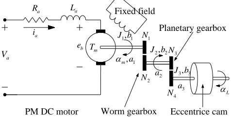
The 3D model of the automatic 3-DOF girder system is shown in Fig. 2. An actuator system is made up of the permanent magnet (PM) DC motor, worm gearbox, planetary gearbox, eccentric circle cam [8], [9], and the rotary encoder. Planetary gearbox can reduce the speed and increase the torque of the PM DC motor [10]. The locked position of the eccentric circle cam is applied by the worm gearbox [11]. In addition, the external disturbances were built by adjusting Bolt-1 and Bolt-2.

Actuator-3

Worm gearbox Eccentric circle cam

Rotary encoder Bolt-1

Actuator-2

Actuator-1

Planetary gearbox

Bolt-2

PM DC motor x

y z

Girder

Fig. 2. 3D model of the automatic 3-DOF girder system

A. Model of the actuator system

Fig. 3 shows the structure of the actuator system. The DC voltage is applied to the armature winding of the motor. The electrical and mechanical characteristics of the system are represented as follows: Va is the armature voltage (V), ia is the armature current (A), R_a is the resistance of winding (Ω),

a

L is the inductance of winding (H), eb is the back electromotive force (V), Kb is the back electromotive force coefficient (V.s/rad), Kt is the motor torque coefficient (N.m/A), Jeq is the moment of inertia of the actuator system (kg.m2_),

eq

b is the viscous friction coefficient of the actuator system (N.m.s/rad), m is the motor velocity (rad/s), Tm is the motor torque (N.m), and TL is the loadtorque (N.m).

a V

a

R La

b e

1, 1 J b

1 , m a



a i

L



1 N

2 N

PM DC motor Worm gearbox Eccentrice cam

Fixed field

2, 2 J b

3, 3 J b

Planetary gearbox

2 a

3 a 3 N

4 N m

T

Fig. 3. The structure of the actuator system

The electrical and mechanical equations are given by

( ) ( ) ( ) ( )

a a a a a b

V t R i t L i t e t (1)

( ) ( )

b b m

e t K t (2)

( ) ( )

m t a

T t K i t (3)

1 m( ) 1 m( ) 1( ) m( )

J



t b



t T t T t (4)

The ratio of gears of worm gearbox and planetary gearbox are

2 1

w

N N N , NpN4 N3, and NtN Nw p. The angular position of shafts are a1N aw 2, a2N ap 3, and a3L. The torques transmitted on gears are T2N Tw1 and T4N Tp 3.

1 1 1 1 1

( ) ( ) ( ) ( )

m

T t J a t b a t T t (5)

2( ) 2 2( ) 2 2( ) 3( )

T t J a t b a t T t (6)

4( ) 3 3( ) 3 3( ) L( )

T t J a t b a t T t (7)

Refer to (6), it can be written as

3( ) w 1( ) p 2 3( ) p 2 3( )

T t N T t N J a t N b a t (8)

Substituting (8) into (7)

 

2

 

2

1 2 3 2 3 3 3 3 3

t P P L

N T  N J a  N b a J a b a T (9)

Substituting (5) into (9)

3( ) 3( ) ( ) ( )

eq eq L t m

J a t b a t T t N T t (10)

2 2 2

3 2 1

2 2 2

3 2 1

( ) ( ) ( )

eq p w p

J J N J N N J

b b N b N N b

  

This _L is the actuator system velocity (rad/s), _m is the angular position of the motor (rad) and L is the angular position of the actuator system (rad). Refer to (1), (10) it can be written as

( ) ( ) ( ) ( )

a a a a a t b L

V t R i t L i t N K  t (11)

( ) ( ) ( )

eq L eq L L t t a

J



b



t T t N K i t (12)

B. Model of the 3-DOF girder system

The coordinate system used to describe the girder movement is shown in Fig. 4. The movement in three-dimensional space are translations along the x-axis (sway, u), y-axis (heave, v), and z-axis (surge, w) and rotations around the x-axis (pitch, θ), y-axis (yaw, ψ), and z-axis (roll, ϕ).

v





Pitch ( ) Yaw ( ) Roll ( )

  



u w Sway ( )

Heave ( ) Surge ( )

u v w

x y

z

Girder System

Fig. 4. The girder coordinate system

(3)

1 0 0

( ) 0 cos sin

0 sin cos

x

R   

 

 

 

_  _

 

 

(13)

cos 0 sin

( ) 0 1 0

sin 0 cos

y R

 



 

 

 

  

 

 

(14)

cos sin 0

( ) sin cos 0

0 0 1

z R

 

  



 

 

  

 

 

(15)

Therefore, the rotation matrix of the girder system is

( ) ( ) ( )

z y x

RR  R  R  and defined as cosc, sins, cos c , sins, cosc, and sins is given by

c c c s s c s s s c c s

c s c c s s s c s s c s

s c s c c

R

                       

    

 

 

 

_   _

 

 

(16)

Drawing of the 3-DOF girder system is shown in Fig. 5. The three actuators will be rotating in the x-y plane and the angle of rotation of the Actuator-1, Actuator-2, and Actuator-3 are 1, 2, and 3 within 90ºrange, respectively. Point A is

the rotation axis, point B is the center of the eccentric circle cam, and point C is the contact point between the eccentric circle cam and the girder. The angle 1, 2, and 3 are 135º ,

135º, and 45º , respectively. The diameter of the eccentric circle cam is 100 mm and the eccentricity (e) is 5 mm. Vector m is the vector from point O (center of the girder) to point A. vector e is the vector from point A to point B. And vector rn is the vector from point B to point C.

45 °

50

5 45

°

254

112

254

112

220 220

x z y

A

B

C

3



3



1, 2

 

1, 2

 

Actuator-1

Actuator-2

Actuator-3

Front view

Side view

Actuator-1, 2

Actuator-3

x z

y

O

rn

e

m

Fig. 5. Drawing of the 3-DOF girder system

The experimental results of a 3-DOF girder system [12] it can be seen that the angle of pitch and roll are small in radians

, 1

  . Therefore, we obtain the small angle approximation are cos1, sin  , cos1, and sin  . Refer to (16), the rotation matrix of a 3-DOF girder system can be written as

1 0

1

0 1

linear R



 





 

 

_  _

 

 

(17)

When the girder system is moving from the ideal vector x_o to the new vector x. Therefore, the transformation matrix consists of the rotation matrix first, followed by the translation matrix. The transformation matrix is given by

1 0 0

1

0 1 0

o o o

x x

y y v

z z



 



  

     

 

  _ _  _ 

 

     

 

     

      

(18)

Then o is the ideal angle of point C, eo is the ideal eccentric vector as e_oe



cos_o sin_o 0



T, and no is the normal vector as no



coso sino 0



T. Vector c is the vector from point O to point C is given by (19). When the girder system is misaligned it can be written as (20) [13].

t

c   m e rn (19)

(cs n). 0 (20)

Normally, vector s_o is defined as vector c_oand the girder system is misaligned s_oc_o. The vector e_t is given by

cos sin

sin

t linear o

e R e e

  

  

 



 

 

  _  _

 

 

(21)

Substituting(19) and (21) into (20), the result as

. . .

t o

e ns nm nr (22)













. .

cos sin cos

cos sin . sin

sin 0

cos cos sin sin

cos sin sin cos

cos( ) sin( )

t o

o o

lhs e n

e

   

   

 

   

          





   

   

 _  _{ } _

   

   

  



   









. ( ). .

cos cos cos

. sin sin . sin

0 0 0

cos sin cos( )

o o o o

y _o _o _o

x z o o o

y

y o x z o o o

rhs m m n e n

m

m m v e

m

m m m v e

 _ _ _

    



      

  



 _{ } _ _ _{ } _

 _{ } _ _ _{ } _

_   _{ } _ _ _{ } _

 _{ }_ __ __ _{ }_{ } __

 

      

(4)



 







sin sin

sin cos sin( )

cos( )

oi zi oi

xi oi yi oi i oi i oi

v m

m m e

e

  

    

 

 

  

 

(23)

1 1 1 1 1

2 1 2 2 2

3 1 3 3

s s 1) cos( )

s s 2 cos( )

s s 3 cos( 3 )

o z o o

m g v e

m g e

   

    

    



    

 _{  } _ 

    

  _{ }   

   

(24)

1 1 1 1 1 1

2 2 2 2 2 2

3 3 3 3 3 3

1 sin cos sin( )

2 sin cos sin( )

3 sin cos sin( )

x o y o o

g m m e















   

Refer to (22), the small angle approximation are sin and

1cos



, it can be written as









. cos( ) cos sin( ) sin

cos( )

t o o o

o

e n e

e

     

  

   

   (25)

Substituting (25) into (22), the result as





cos





sin

cos( )

yi oi xi zi oi i oi

m m m v

e

    

  

   

   (26)

Therefore, the inverse kinematics equation of a 3-DOF girder system is given by













1 1 1 1 1

1

1 1

2 2 2 2 2

1

2 2

3 3 3 3 3

1

3 3

cos sin

cos

cos sin

cos

cos sin

cos

y x z

m m m v

e

m m m v

e

m m m v

e

    

  

    

  

    

  



    

    

 

 

    

    

 

 

    

    

 

 

(27)

III. THE CONTROL SYSTEM DESIGN

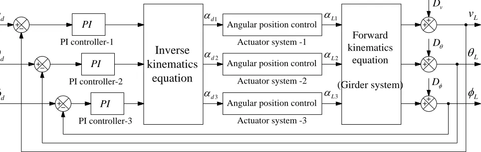
The new technique of the control system design of the automatic 3-DOF girder system consists of two control loops: a) the inner control loop which is composed of three actuator systems and b) the outer control loop which tracks the reference input and regulates the output response of the heave, pitch, and roll of the girder system. Block diagram of the control system of the automatic 3-DOF girder system is shown in Fig. 6. The reference input are the heave (v_d), pitch (_d), and roll (_d ). The angular position input of three actuator systems are _d₁, _d₂, and _d₃ which calculated by the inverse kinematics equation and the angular position output are _L₁, _L₂, and _L₃. The output response are heave (v_L), pitch (_L), and roll (_L). The external disturbances of the 3-DOF girder system are D_v, D_, and D_.

A. The angular position control of the actuator system

The angular position control of the eccentric circle cam actuator system is actuated by a PM DC motor, worm gearbox, and planetary gearbox. Measured the angular position by the rotary encoder. The control system uses the state feedback control with the full-order state observer based on the pole placement method [14], [15]. Therefore, the control system design as follows:

( ) ( ) ( )

( ) ( )

t t u t

y t t

 



x Ax B

Cx (28)

Where x( )t is the state vector and define the state variables are x₁



L( )t , x2L( )t , and x3i ta( ). A, B, and C are

constant matrices. u t( ) is the control signal equal to V t_a( ).

( )

y t is the output signal equal to L( )t . Refer to (11), (12),

we obtain the state equation is given by

( ) ( )

( )

( ) ( ) ( )

( )

L L

eq L t t a L

eq eq t b L a a a a

a a a

t t

b t N K i t

t

J J

N K t R i t V t

i t

L L L

 

 





  

   

(29)

The state space equations can be written by





0 1 0

0

0 0

1 0

1 0 0

L L

eq t t

L L a

eq eq

a a

t b a

a a a

L L a

b _{N K}

V

J J

i i

N K R _L

L L

y

i

 

 

 

 

   

   

  _ _  _ _

 __ _ _ _{ } _

  _ _  _ _

   

      

 _ _  _ _

 

 

 

 

 _ _

 

 

(30)

A prototype of the actuator system is shown in Fig. 7. The prototype consists of a PM DC motor, worm gearbox with gear ratio 15:1, planetary gearbox with gear ratio 50:1, eccentric circle cam, and the rotary encoder which has 2,500 pulses per revolution. We use the multi-meter and LCR meter to measure the resistance and inductance of the motor winding

3.2715 a

R  Ω and L_a2.0487 10 3H. And estimating the value of parameters are Kb, Kt, Jeq, and beq is based on measuring the output velocity of the eccentric circle cam. The parameter estimation of the actuator system using MATLAB-Simulink based on the simplex search method [16]

2

7.0103 10 b

K    V.s/rad, _{9.5361 10}3

t

K    N.m/A,

14.7729 eq

J  kg.m2_{, and} _5.8634

eq

(5)

PI L

v

L



L



v

D

D_

D_

d

v

d



d



1

d



2

d



3

d



2

L



1

L



3

L



Inverse

kinematics

equation

Forward kinematics

equation

(Girder system)

Angular position control

Angular position control PI controller-1

PI controller-3 PI controller-2

PI

Actuator system -1

Actuator system -2

Actuator system -3

Fig. 6. Block diagram of the control system of the automatic 3-DOF girder system

PM DC motor

Worm gearbox Planetary gearbox

Eccentric circle cam

Rotary encoder

Girder

Fig. 7. Prototype of the actuator system

Refer to (30), it can be rewritten as





1 1

2 2

3 3

1

2

3

0 1 0 0

0 0.3969 0.4841 0

0 25, 663.7135 1, 596.8663 488.1144

1 0 0

x x

x x u

x x

x

y x

x

      

 _ _  _ 

      

  _   _  _ _

   

   

 _{ }

   

(31) Hence, the transfer function of the actuator system







( ) 236.2961

( ) 1,589.0453 8.2178

L a

s

V s s s s

 

 

Then the system is type 1 with involves the integral. Block diagram of the state feedback control is shown in Fig. 8.

The control signal is determined by

u Kx (32)













1

2 3 2 1 1

3

1 1 2 2 3 3 1 1

0 _d

d d

x

u k k x k x

x

k x k x k x k k



 

   

  _{ } 

   

      Kx

+ u



x Ax B

3

k

2

k

d



u x1



L

yCx

3

x

2

x

1

k

1

x

Fig. 8. Block diagram of the state feedback control

K is the state feedback gain matrix. And the controllability matrix of the actuator system is given by

2

 

 

M = B AB A B (33)

The determinant of matrix M is 2.7258 10 7, so the rank of the controllability matrix is equal to the rank of the system. Therefore, the actuator system completely states controllable.

The desired of the closed-loop poles of the angular position control at p₁  4 3j, p₂  4 3j, and p₃ 2, 000. Then the damping ratio of the actuator system is  0.8 and undamped natural frequency is _n 5 rad/s. Characteristic

equation is 3 2

2,008 16,025 50,000

s  s  s . The Ackermann's

formula [14] for determining the state feedback gain matrix is given by





₂ 1

 

0 0 1_ _ 

K = B AB A B A (34)

Since

 

3 2

2,008 16,025 50,000

 A A  A  A I. Therefore,

the state feedback gains are k₁211.5988, k₂=11.8681, and

3 0.8415

k  .

(6)

2,3

k

L B

A

C

d 

y

x x B

A

C 

1

k u L

Full-order state observer



Fig. 9. Block diagram of the observer-based state feedback control

The full-order state observer equation is given by





( ) ( ) ( ) ( ) ( )

( ) ( )

t t u t y t t

u t t

   

 

x Ax B L Cx

Kx

(35)

( )t

x is the estimated state vector, Cx( )t is the estimated output signal. The output signal and the control signal are input to the observer. Matrix L is the observer gain matrix that correcting disparity between the measured output signal and estimated output signal.

Refer to (35), the Laplace transform is given by





1

( ) ( )

s s Y s

U s s



   

 

X I A LC BK L

KX

(36)

The transfer function of the observer-based state feedback control is given by





1

( ) ( ) U s

s Y s



   

 K I A LC BK L (37)

The observability matrix of the actuator system is given by

2

 

 

 

C

O = CA

CA

(38)

The determinant of matrix O is 0.4814 , so the rank of the observability matrix is equal to the rank of the system. Therefore, the actuator system completely states observable.

The desired of the closed-loop poles of the observer at

4 500 500

p    j, p₅ 500 500 j, and p₆ 2, 000. Then the damping ratio of the observer system is  0.7 and undamped natural frequency is _n707 rad/s. The characteristic equation of the observer system is

3 3 2 6 9

3 10 2.5 10 1 10

s   s   s  . The Ackermann's formula

[14] for the state observer gain matrix is given by

 

1

2

0 0 1 



 _{  }

 _{  }

 _{  }_{ }

 

C

L = A CA

CA

(39)

Since 

 

A A3 3 103A22.5 10 6A 1 109I.

Therefore, the state observer gains are l₁=1, 402.7368,

2 246, 402.5301

l  , and l₃=1, 214,975, 450.6596. Refer to (37), the transfer function of the observer-based state feedback control is given by

9 2 9 11

3 3 2 6 9

( ) 1.03 10 10 10

( ) 3.41

7.

10 3.08 10 1.1

27 2.

1 2

10 1

U s s s

Y s s s s

    



      

See Fig. 7 and Fig. 9, _d is the angular position input (reference input) and L is the angular position output (output

response). Therefore, the experimental results of the angular position control of the actuator system are shown in Fig. 10. Fig. 10(a) shows the angle of rotation with +90º and Fig. 10(b) illustrates the angle of rotation within +90º range. We can see the errors between the reference input and the output response is very small within the ±0.20º range.

(a) The angle of rotation with +90°

(b) The angle of rotation within +90° range

0 10 20 30 40 50 60 70 80 90 100

0 20 40 60 80 100

An

g

u

la

r

p

o

si

ti

o

n

(d

e

g

)

Time (sec)

Reference input Output response

0 10 20 30 40 50

0 20 40 60 80 100

An

g

u

la

r

p

o

si

ti

o

n

(d

e

g

)

Time (sec)

Fig. 10. Experimental results of the angular position control of the actuator system

B. The motion control of the 3-DOF girder system

(7)

Given initail Kp, Ki gains (heave, pitch and roll)

Simulation

Automatic 3-DOF girder system (heave, pitch and roll) Set bounds for the output response

(heave, pitch and roll) by step response characteristics

Checked the output response (heave, pitch and roll)

Extracted Kp, Ki gains (heave, pitch and roll) No

Yes Start

End Optimization

Kp, Ki gains

Fig. 11. Flowchart of the optimization method for the PI controller gains

The optimization method for the PI controller gains Kp

and K_i is presented as follows:

Step-1 (K_p₁ and K_i₁ gains): Given the initial conditions of

1, 1, 2, 2, 3

p i p i p

K K K K K and Ki3 gains of the PI controller 1,

PI controller 2, and PI controller 3. Setting the bounds of the output response for the heave (pitch and roll equal to zero), the final value +5 mm, rise time 5 sec, overshoot 5 %, settling time 8 sec, and steady-state error ±0.2 %. Simulation of the automatic 3-DOF girder system (see Fig. 6). Checked the output response of the heave (the error between the setting bounds and the output response). Therefore, the PI controller gains are K_p₁0.1654 and Ki₁0.4603.

Step-2 (K_p₂ and K_i₂ gains): Given the initial conditions of

2, 2, 3

p i p

K K K , and K_i₃ gains of the PI controller 2 and PI controller 3. Setting the bounds of the output response for the pitch (heave and roll equal to zero), the final value +20 mrad, rise time 5 sec, overshoot 5 %, settling time 8 sec, and steady-state error ±0.2 %. Simulation and checked the output response of the pitch. Therefore, the PI controller gains are

2 0.1809

p

K  and Ki₂0.5223.

Step-3 (K_p₃ and K_i₃ gains): Given the initial conditions of

3

p

K and K_i₃ of the PI controller 3. Setting the bounds of the output response for the roll (heave and pitch equal to zero), the final value +20 mrad, rise time 5 sec, overshoot 5 %, settling time 8 sec, and steady-state error ±0.2 %. Simulation and

checked the output response of the roll. Therefore, the PI controller gains are K_p₃0.2223 and Ki₁0.7689.

IV. THE EXPERIMENTAL RESULTS

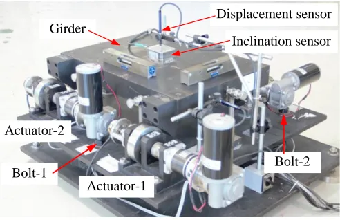
In-house fabricated prototype and the experimental setup of the automatic 3-DOF girder system is shown in Fig. 12 (see Fig 2). The girder system is based on three eccentric circle cam actuators are Actuator-1, Actuator-2, and Actuator-3 and the weight of the girder about 100 kg. The translation along the y-axis (heave) is measured by a displacement sensor which has an accuracy of 0.005 mm. The rotation around the x-axis (pitch) and the z-axis (roll) are measured by an inclination sensor which has an accuracy of 0.6 mrad. The sensors are installed at the center of the girder. The automatic 3-DOF girder system has been tested by the RAPCON platform [20], [21] with MATLAB-Simulink. The inner control loops use three actuator systems with the observer-based state feedback control. The outer control loops use the tracking control and output regulation with the PI controller 1, PI controller 2, and PI controller 3 in which use K_p and K_i values derived from the optimization.

Displacement sensor

Inclination sensor

Actuator-1 Girder

Actuator-2

Bolt-2 Bolt-1

Fig. 12. Prototype of the automatic 3-DOF girder system

A. The tracking control

See Fig. 2, Fig. 6, and Fig. 12, the experiment results of the tracking control are shown in Fig. 13 - Fig. 15 without the external disturbances (D_v, D_, and D_). In Fig. 13(a) - Fig. 15(a) shows the step reference input and the output response of the heave is +5 mm, of the pitch is +20 mrad and of the roll is +20 mrad, respectively. In Fig. 13(b) - Fig. 15(b) shows the angle of rotation of three actuator systems (see Fig. 9,

Alpha-dd and Alpha-LL). We can see the settling

(8)

(a) Translation along the y-axis (+5 mm)

(b) Angle of rotation of three actuator system

5 10 15 20 25 30

0 1 2 3 4 5 6

H

e

a

ve

(mm)

Time(sec)

5 10 15 20 25 30

-60 -40 -20 0

(Actuator-1)

5 10 15 20 25 30

-60 -40 -200

An

g

u

la

r

p

o

si

ti

o

n

(d

e

g

)

(Actuator-2)

5 10 15 20 25 30

0 20 40 60

Time(sec) (Actuator-3)

Alpha-d Alpha-L

Fig. 13. The translation along the y-axis (heave) with +5 mm

(a) Rotation around the x-axis (+20 mrad)

(b) Angle of rotation of three actuator system

5 10 15 20 25 30

-60 -40 -200

(Actuator-1)

5 10 15 20 25 30

0 20 40 60

An

g

u

la

r

p

o

si

ti

o

n

(d

e

g

)

(Actuator-2) _Alpha-d

Alpha-L

5 10 15 20 25 30

-20 0 20 40

5 10 15 20 25 30

0 5 10 15 20 25

Pi

tch

(mra

d

)

Time(sec)

Fig. 14. The rotation around the x-axis (pitch) with +20 mrad

(a) Rotation around the z-axis (+20 mrad)

(b) Angle of rotation of three actuator systems

5 10 15 20 25 30

0 5 10 15 20 25

R

o

ll

(mra

d

)

Time(sec)

5 10 15 20 25 30

-60 -40 -200

(Actuator-1)

5 10 15 20 25 30

-60 -40 -200

An

g

u

la

r

p

o

si

ti

o

n

(d

e

g

)

(Actuator-2)

Alpha-d Alpha-L

5 10 15 20 25 30

-60 -40 -200

Fig. 15. The rotation around the z-axis (roll) with +20 mrad

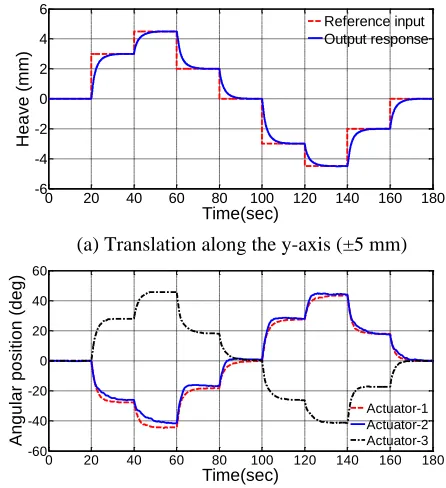
See Fig. 2, Fig. 6, and Fig. 12, the experiment results of the tracking control are shown in Fig. 16 - Fig. 18 without the external disturbances. In Fig. 16(a) - Fig. 18(a) shows the girder system can track the step reference input of the heave within ±5 mm range, of the pitch and roll within ±20 mrad range, respectively. In Fig. 16(b) - Fig. 18(b) shows the angle of rotation of three actuator systems. We can see the 3-DOF girder system can exactly and quickly tracks the reference input of the heave, of the pitch, and roll.

(a) Translation along the y-axis (±5 mm)

0 20 40 60 80 100 120 140 160 180 -60

-40 -20 0 20 40 60

An

g

u

la

r

p

o

si

ti

o

n

(d

e

g

)

Time(sec)

Actuator-1 Actuator-2 Actuator-3 0 20 40 60 80 100 120 140 160 180 -6

-4 -2 0 2 4 6

H

e

a

ve

(mm)

Time(sec)

(9)

(a) Rotation around the x-axis (±20 mrad)

(b) Angle of rotation of three actuator systems 0 20 40 60 80 100 120 140 160 180 -24

-16 -8 0 8 16 24

Pi

tch

(mra

d

)

Time(sec)

0 20 40 60 80 100 120 140 160 180

-60 -40 -20 0 20 40 60

An

g

u

la

r

p

o

si

ti

o

n

(d

e

g

)

Time(sec)

Actuator-1 Actuator-2 Actuator-3

Fig. 17. Tracking control of the rotation around the x-axis (pitch) within ±20 mrad range

(a) Rotation around the z-axis (±20 mrad)

0 20 40 60 80 100 120 140 160 180

-60 -40 -20 0 20 40 60

An

g

u

la

r

p

o

si

ti

o

n

(d

e

g

)

Time(sec)

0 20 40 60 80 100 120 140 160 180 -24

-16 -8 0 8 16 24

R

o

ll

(mra

d

)

Time(sec)

Fig. 18. Tracking control of the rotation around the z-axis (roll) within ±20 mrad range

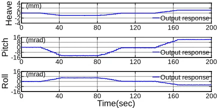
B. The output regulation

The prototype of a 3-DOF girder system can exactly track the reference input of the heave, pitch, and roll without the external disturbances. See Fig. 2, Fig. 6, and Fig. 12, the external disturbance signals (D_v, D_, and D_) were built by adjusting Bolt-1 and Bolt-2 (the control system do not use). Therefore, the external disturbance signals were built by adjusting Bolt-1 and Bolt-2 is shown in Fig. 19 and Fig. 20.

0 40 80 120 160 200

-4 -20 2 4

H

e

a

ve (mm)

0 40 80 120 160 200

-16-8 0 8 16

Pi

tch (mrad)

0 40 80 120 160 200

-16-8 0 8 16

Time(sec)

R

o

ll (mrad)

Output response

Fig. 19. The external disturbance signals were built by adjusting Bolt-1

0 40 80 120 160 200

-4 -20 2 4

H

e

a

ve (mm)

0 40 80 120 160 200

-16-8 0 8 16

Pi

tch (mrad)

0 40 80 120 160 200

-16-8 0 8 16

Time(sec)

R

o

ll (mrad)

Output response

Fig. 20. The external disturbance signals were built by adjusting Bolt-2

The experiment results of the output regulation are shown in Fig. 21 and Fig. 22 with the external disturbances signals were built by adjusting Bolt-1 (see Fig. 19) and adjusting Bolt-2 (see Fig. 20). In Fig. 21(a) and Fig. 22(a), shows the output response of the heave, the pitch, and roll with setting the reference input of the heave, the pitch, and roll to zero with adjusted Bolt-1 and adjusted Bolt-2. In Fig. 21(b) and Fig. 22(b), shows the angle of rotation of three actuator systems. We can see the 3-DOF girder system can robustly regulate the output response of the heave, the pitch, and roll to zero.

(a) Output responses of heave, pitch, and roll

(b) Angle of rotation of three actuator systems (b) Angular position of the actuator system

0 40 80 120 160 200

-4 -20 2 4

H

e

a

ve (mm)

0 40 80 120 160 200

-16-8 0 8 16

Pi

tch (mrad)

0 40 80 120 160 200

-16-8 0 8 16

Time(sec)

R

o

ll (mrad)

Output response

0 40 80 120 160 200

-60 -40 -20 0 20 40 60

An

g

u

la

r

p

o

si

ti

o

n

(d

e

g

)

Time(sec)

(10)

(a) Output responses of heave, pitch, and roll

(b) Angle of rotation of three actuator systems (b) Angular position of the actuator system

0 40 80 120 160 200

-4 -20 2 4

H

e

a

ve (mm)

0 40 80 120 160 200

-16-8 0 8 16

Pi

tch (mrad)

0 40 80 120 160 200

-16-8 0 8 16

Time(sec)

R

o

ll (mrad)

Output response

0 40 80 120 160 200

-60 -40 -20 0 20 40 60

An

g

u

la

r

p

o

si

ti

o

n

(d

e

g

)

Time(sec)

Fig. 22. Output regulation with the disturbance signals were built by adjusting Bolt-2

V. CONCLUSION

This paper presents the new technique of the control system design of the automatic 3-DOF girder system for aligning the magnets in the electron storage ring. The prototype of the girder system has been built to demonstrate the effectiveness of the mathematical models, angular position control of the actuator system, tracking control and output regulation of the girder system. The experimental results reveal that the actuator system can precisely track the reference input with an accuracy ±0.20º, the girder system can exactly and quickly track the reference input of the heave with an accuracy ±0.01 mm, the pitch and roll with an accuracy ±0.6 mrad and can robustly regulate the output response which has the external disturbances. In addition, the girder system can successfully perform the design values of the heave within ±5 mm range, the pitch and roll within ±20 mrad range. Therefore, this prototype is appropriate for developing the magnet girder system for plane stabilization of the electron storage ring. For future research, the automatic girder system with higher degrees of freedom and higher precision will be designed.

ACKNOWLEDGMENT

The authors would like to acknowledge the support of Suranaree University of Technology (SUT) and this work was financially supported by the Ministry of Science and Technology (MOST) and the Synchrotron Light Research Institute (SLRI) of the Royal Thai Government.

REFERENCES

[1] P.C.D. King, R.H. He, T. Eknapakul et al., “Subband structure of a two-dimensional electron gas formed at the polar surface of the strong spin-orbit perovskite KTaO3,” Physical Review Letters, vol. 108, pp.

117602-1-117602-5, 2012.

[2] R. Gosalawit-Utke, S. Meethom, C. Pistidda et al., “Destabilization of LiBH4 by nanoconfinement in PMMA-co-BM polymer matrix for

reversible hydrogen storage,” International Journal of Hydrogen Energy, vol. 39, pp. 5019-5029, 2014.

[3] S. Sonsupap, P. Kidkhunthod, N. Chanlek et al., “Fabrication, structure, and magnetic properties of electrospun Ce0.96Fe0.04O2 nanofibers,” Applied Surface Science, vol. 380, pp. 16-22, 2016.

[4] N. Sanguansak, S. Matsui, S. Rujirawat et al., “Realignment magnets of Siam Photon Source storage ring,” in Proceedings of 7th International Workshop on Accelerator Alignment, pp. 55-58, Spring-8, Japan, 2002. [5] S. Srichan, A. Kwankasem, S. Boonsuya et al., “Status report on storage

ring realignment at SLRI,” in Proceedings of 12th International Workshop on Accelerator Alignment, Fermilab, USA, 2012.

[6] S. Zelenika, R. Kramert, L. Rivkin et al., “The SLS storage ring support and alignment systems,” Nuclear Instruments and Methods in Physics Research A, vol. 467-468, pp. 99-102, 2001.

[7] I.P. Martin, A.I. Bell, A. Gonias et al., “Diamond storage ring remote alignment system,” in Proceedings of 10th European Particle Accelerator Conference, pp. 523-525, Edinburgh, Scotland, 2006. [8] H.A. Rothbart (Eds.), Cam Design Handbook, McGRAW-HILL, New

York, 2004.

[9] J. Kemppinen, F. Lackner, and H.M. Durand, “Validation test of a cam mover based micrometric pre-alignment system for future accelerator components,” Measurement Science Review, vol. 12, pp. 162-157, 2012. [10] T. Schulze, C. Hartmann, and B. Schlecht, “Calculation of load distribution in planetary gears for an effective gear design process,”

American Gear Manufacturers Association, Technical Resources 10FTM08, pp. 1-11, 2010.

[11] A.L. Kapelevich, and E. Taye, “Self-locking gears: Design and potential applications,” American Gear Manufacturers Association, Technical Resources 10FTM17, pp. 3-8, 2010.

[12] S. Prawanta, S. Khaengkarn, and J. Srisertpol, “Motion control of a 3-DOF girder system using eccentric circular cam,” in Proceedings of Asia-Pacific Conference on Intelligent Robot Systems, pp. 132-136,

Tokyo, Japan, 2016.

[13] A. Sterm, “Algorithms for dynamic alignment of the SLS storage ring girders,” Paul Scherrer Institut, SLS-TME-TA-2000-0152, Villigen PSI, Switzerland, 2000.

[14] K. Ogata, Modern Control Engineering, PEARSON, New York, 2010. [15] S.N. Norman, Control System Engineering, John Wiley & Sons, USA,

2011.

[16] W. Koech, T. Rotich, F. Nyamwala et al., “Parameter estimation of a DC motor-gear-alternator system via step response methodology,”

American Journal of Applied Mathematics, vol. 4, no. 5, pp. 252-257, 2016.

[17] M.A. Johnson, and M.H. Moradi, PID Control New Identification and Design Methods, Springer, London, 2005.

[18] N. Tippayawannakorn, and J. Pichitlamken, “Nelder-Mead method with local selection using neighbourhood and memory for stochastic optimization,” Journal of Computer Science, vol. 9, no. 4, pp. 463-476, 2013.

[19] B. Nayak, and T. R. Choudhury, “Optimization of PI coeffecients of permanent magnet synchronous motor drive,” Indian Journal of Science and Technology, vol. 10, no. 25, pp. 1-11, 2017.

[20] W. Wiboonjaroen, and S. Sujitjorn, “Stabilization of a magnetic levitation control system via state-pi feedback,” International Journal of Mathematical Models and Method in Applied Sciences, vol. 7, pp. 717-727, 2013.

[21] RAPCON (Rapid Control Platform for MATLAB-Simulink) www.zeltom.com/products/rapcon

Supachai Prawanta was born in Khon Kaen, Thailand, in 1974. He received the B.Eng. and M.Eng. in the School of Electrical Engineering from Suranaree University of Technology (SUT), Thailand, in 1997 and 2008. He is currently a Ph.D. candidate in the School of Mechanical Engineering at SUT.