ESTIMATION OF DESIGN FLOOD WITH FOUR FREQUENCY ANALYSIS DISTRIBUTIONS

(1)

Estimation of Design Flood with Four Frequency Analysis Distributions

Ery Suhartanto

1

, Lily Montarcih Limantara

1

, Dina Noviadriana

2

, Febri Iman Harta

2

and Dwi Aryani K

2

1_{Lecturer on the Department of Water Resources, Faculty of Engineering, University of Brawijaya, Jl. MT Haryono No. 167 Malang 65145, East Java of} Indonesia.

2

Doctoral Program on the Department of Water Resources, Faculty of Engineering, University of Brawijaya, Jl. MT Haryono No. 167 Malang 65145, East Java of Indonesia

Article Received: 21 September 2017 Article Accepted: 23 December2017 Article Published: 07 January 2018

1. INTRODUCTION

Frequency analysis is generally used in hydrology for the possibility of discharge extremes, mainly for low flow or

high flow [1]. .The application of the frequency analysis methods has been widely recognized by the numerous

researchers in the field. There are several kinds of frequency analysis distribution that have been successfully

applied to the hydrological data [2]. Some of the extreme value probability distributions are usually used for

hydrological analysis such as Normal Distribution, Log-Normal Distribution, Gumbel-Weibull Distribution, and

Log Perason Type III Distribution [3].

Flood frequency analysis is the important parameter to determine the extend od flooding for the different of return

period [4]. Generally, the instantaneous peak discharge of river at the various recorded location are taken from long

term data [5] and the maximum flood of each year is extracted. Then the data is processed for the outliers and

consistency test. The outliers is those the data points which departs significantly from the trend of the remaining

data [6]. The consistency of data is evaluated with the help of t-test (t-statistics) [7]. Estimation of design flood are

routinely required by water resources engineering purposes. The design flood is required for the planning and

operation measures, the structural design, and the safety and risk analysis of the existing structures [8]. The

conventional approaches for estimating the design flood are the flood frequency analysis. Hosking [9] and Hosking

and Wallis [10] have provided the estimation of design floods based on the regional frequency analysis. However,

Moon and Lall [11] used the nonparametric kernel estimator for reliable flood frequencies estimation analysis.

The Lesti sub-watershed is located in the Malang regency and it is as the priority sub-watershed in the upstream

Brantas watershed. The Lesti sub-watershed has the complex enough of problem related with the area damage,

erosion, landslide, the fluctuation of river discharge and sedimentation is high enough. In the last few years, the

condition is changed regarding to the land use change, geographical condition of the upstream area where is part of

A B S T R A C T

The Lesti sub-watershed has the complex enough of problem related with the area damage, erosion, landslide, the fluctuation of river discharge and sedimentation is high enough. The solution which can be carried out to prevent the problem is by the accurate design, develop ment, and the controlling of water structure accurately. However, the accuracy can be reached by the optimum accuracy in analyses including the hydrological analysis in it. One of the important hydrological analyses is to calculate the design flood. This study intends to analyze the design flood by using the four frequency analysis distribution. The methodology consist of analyzing the flood frequency by using the distributions of Normal, Log Normal, Log Pearson Type III, and Gumbel. The result is hoped can support the accurate project design of water resources structures.

(2)

them is as mountainous, the global climate change, and the dangerous level of natural disaster in the Lesti

sub-watershed is high enough.

The solution to prevent the problem is by well design, development, and controlling the water structure accurately.

However, the accuracy can be reached by the optimum accuracy in analyses including the hydrological analysis in

it. One of the important hydrological analysis is to calculate the design flood. Therefore, the analysis of design

flood is very necessary to be carried out including the testing of goodness of fit for evaluating the suitable

probability distribution which is used in the frequency analysis. In additional, this evaluation is also to know the

suitable water recorder as the reference of flooding recorder.

2. MATERIALS AND METHODS

2.1. Study location

Lesti sub-watershed is located on the south longest of 8°02’50’’- 8°12’10’’ and east longest of 112° 42’58’’-

112°56’21’’. This area is on the Malang regency and has the heterogenic characteristic of the basic physical

condition. The delineation of the research area uses the ecological boundary such as the division of the upstream

Lesti sub-watershed which is remained by the Brantas watershed determination institution.

The condition of river network is known that the Lesti sub-watershed has the river arbitrary with the tree shaped

which the affluent connects to the main river. The pattern shows that part of the area is homogeny. It indicates that

there is happened the concentration of water surface in this area. However, this condition will cause the ability of

water absorption in the soil is relatively small so it will be frequently happened the flooding and there is the water

concentration (flooding) in some area. Map of the study location is presented as in the Figure 1.

(3)

2.2. Data collecting

The secondary data are needed for this study. The secondary data are the data which is obtained from some sources

which can be responsible to the truth. The secondary data which are needed in this study is as follow:

1. The daily rainfall data from the Poncokusumo station (2007-2016)

2. The daily rainfall data from the Dampit station (2007-2016)

3. The daily discharge data from the Tawangrejeni water recorder (2007-2016)

2.3. Steps of study

The steps of study are as follow:

1. To analyze the design flood by using the methods of Normal, Log Normal, Log Perason Type III. And Gumbel.

2. To carry out the testing of goodness of fit by using the methods of smirnov-kolmogorof and chi-square.

2.4. Normal distribution

The Normal distribution or Normal curve is also mentioned as the Gauss distribution. The formula for calculating

the estimation value with the return period of T (Xt) is as follow:

(1)

Where,

XT : estimation of value which is hoped to be happened by the return period of T

X : mean

S : deviation standard

KT : factor of frequency which is as the function of probability or return period and as the type of mathematical

modeling of the probability distribution that is used for the probability analysis

2.5. Log Normal distribution

The formula of Log Normal distribution is the same as the Normal distribution, but the data have to be transformed

(4)

(2)

Where,

XT : estimation of value which is hoped to be happened by the return period of T )in the log)

X : mean (in the log)

S : deviation standard (in the log)

2.6. Log Pearson Type III distribution

To use the Log Pearson Type III, the data have to be transformed into the Log form. The formula of Log Pearson

Type III with the return period of T (Xt) is as follow:

Log XT = Log X + K.s (3)

Where,

Log XT : estimation of value (in the Log from) which is hoped to be happened by the return period of T

X : mean (in the Log form)

S : deviation standard (in the log form)

2.7. Gumbel distribution

The formula of the Gumbel distribution that is used for estimating the value which is hoped to be happened with the

return period of T(Xt) is as follow:

(4)

(5)

Xt = design rainfall in the return period of T year (mm)

X = mean rainfall of the observed result

Yt = reduced variate that is as the Gumbel parameter for the return period of T year

Yn = reduced mean that is as the function of the data number= f(n)

Sn = reduced deviation standard that is as the function of the data number = f(n)

Sx = deviation standard

3. RESULTS AND DISCUSSIONS

3.1. Analysis of discharge data

In the hydrological analysis, the data of Automatic Water Level Recorder (AWLR) is obtained from the

Tawangrejeni station which consists of disxharge data on the period from 2007 until 2016. Table 1 presents the

maximum discharge of Tawangrejeni AWLR.

Table 1. Maximum discharge data of Tawangrejeni AWLR

No. Year Discharge (m3/s)

1 2007 514.4

2 2008 202.5

3 2009 254.7

4 2010 85.8

5 2011 127.9

6 2012 175.3

7 2013 86.5

8 2014 81.5

9 2015 72.3

10 2016 63.2

Source: own study

3.2. Analysis by using the Normal Distribution

Analysis by using the Normal distribution uses the formula as follow:

(5)

The data preparation is presented as in the Table 2, however the result of design flood by using the Normal

(6)

Table 2. Data preparation for Normal distribution analysis

No year Q max

(m3/s)

1 2016 63.25

2 2015 72.34

3 2014 81.47

4 2010 85.79

5 2013 86.50

6 2011 127.85

7 2012 175.29

8 2008 202.54

9 2009 254.67

10 2007 514.42

Mean 166.4

Deviation standard 138.0

Source: own study

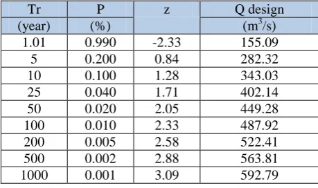
Table 3. Result of design flood by using the Normal distribution

Tr P z Q design

(year) (%) (m3/s)

1.01 0.990 -2.33 155.09

5 0.200 0.84 282.32

10 0.100 1.28 343.03

25 0.040 1.71 402.14

50 0.020 2.05 449.28

100 0.010 2.33 487.92

200 0.005 2.58 522.41

500 0.002 2.88 563.81

1000 0.001 3.09 592.79

Source: own study

Explanation: Tr = return period; P = probability; Z = parameter in Normal distribution; Q = discharge

3.3. Analysis by using the Log Normal distribution

If y = log x, so the analysis by using the Log Normal distribution can be carried out by using the formula of the

Normal distribution. The data preparation for the Log Normal distribution is presented as in the Table 4, however,

the result of design flood by using the Log Normal distribution is presented as in the Table 5.

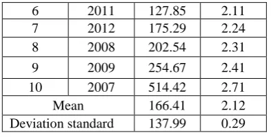
Table 4. Data preparation for Log Normal analysis

No year Q Max Log Q

(m3/s)

1 2016 63.25 1.80

2 2015 72.34 1.86

3 2014 81.47 1.91

4 2010 85.79 1.93

(7)

6 2011 127.85 2.11

7 2012 175.29 2.24

8 2008 202.54 2.31

9 2009 254.67 2.41

10 2007 514.42 2.71

Mean 166.41 2.12

Deviation standard 137.99 0.29

Source: own study

Table 5. Result of design flood by using the Log Normal distribution

Tr P

P(z) z Log Q Q design

(year) (%) (m3/s)

1.01 99 0.010 -2.33 1.44 27.74

5 20 0.800 0.84 2.37 232.41

10 10 0.900 1.28 2.49 312.17

25 4 0.960 1.71 2.62 416.03

50 2 0.980 2.05 2.72 523.15

100 1 0.990 2.33 2.80 631.20

200 0.5 0.995 2.58 2.87 746.41

500 0.2 0.998 2.88 2.96 912.73

1000 0.1 0.999 3.09 3.02 1050.75

Source: own study, Explanation: Tr = return period; P = probability; Q = discharge

3.4. Analysis by using the Log Pearson Type III

If y = log x, so the analysis by using Log Pearson III distribution can be carried out by transforming the data into

Log form and then to analyze it by using the formula of Log Pearson III. The data preparation for the Log Pearson

III distribution is presented as in the Table 6, however, the result of design flood by using the Log Pearson III

distribution is presented as in the Table 7.

Table 6. Data preparation for the Log Pearson Type III distribution

No year Q Max Log Q

(m3/s)

1 2016 63.2 1.80

2 2015 72.3 1.86

3 2014 81.5 1.91

4 2010 85.8 1.93

5 2013 86.5 1.94

6 2011 127.9 2.11

7 2012 175.3 2.24

8 2008 202.5 2.31

9 2009 254.7 2.41

10 2007 514.4 2.71

Mean Log Q 2.12

Cs Log Q 0.92

Deviation standard of Log Q 0.29

(8)

Table 7. Result of design flood by using the Log Pearson Type III distribution

Tr P

K Log Q Q design

(year) (%) (m3/s)

1.01 99 -1.648 1.64 43.81

2 50 -0.151 2.08 119.61

5 20 0.767 2.35 221.34

10 10 1.339 2.51 324.80

25 4 2.022 2.71 513.43

50 2 2.505 2.85 709.85

100 1 2.968 2.99 967.89

200 0.5 3.415 3.12 1306.80

500 0.2 3.791 3.23 1681.78

1000 0.1 4.418 3.41 2560.76

Source: own study

Explanation: Tr = return period; P = probability; k = coefficient of frequency; Q= discharge

3.5. Analysis by using the Gumbel distribution

By using the Gumbel distribution, the data preparation for Gumbel distribution is presented as in the Table 8,

however, the result of design flood by using the Gumbel distribution is presented as in the Table 9.

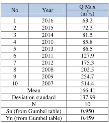
Table 8. Data preparation for Gumbel distribution

No Year Q Max

(m3/s)

1 2016 63.2

2 2015 72.3

3 2014 81.5

4 2010 85.8

5 2013 86.5

6 2011 127.9

7 2012 175.3

8 2008 202.5

9 2009 254.7

10 2007 514.4

Mean 166.41

Deviation standard 137.99

N 10

Sn (from Gumbel table) 0.950 Yn (from Gumbel table) 0.459

Source: own study

Table 9. Result of design flood by using the Gumbel distribution

Tr P

Yt K Q design

(year) (%) (m3/s)

1.01 99 -1.529 -2.094 -122.54

2 50 0.367 -0.098 152.94

(9)

10 10 _2.250 _1.886 _426.68

20 5 2.970 2.644 531.28

25 4 3.199 2.885 564.46

50 2 3.902 3.625 666.67

100 1 4.600 4.361 768.13

200 0.5 5.296 5.093 869.21

500 0.2 6.214 6.060 1002.58

1000 0.1 6.907 6.790 1103.37

Sumber : Hasil perhitungan

Explanation: Tr = return period; P = probability; k = coefficient of frequency; Q= discharge; Yt = reduced variate

3.6. Testing of goodness of fit by using Smirnov Kolmogorov test

Testing of goodness of fit by using Smirnov-Kolmogorof test is carried out by comparing the probability of every

variant between the empirical and theoretical probability and then the maximum deviation is compared with the

deviation of table [12].

If the Δ max (D max) on the probability paper is less than Δ critic (Dcr) for a level of significance and the number

of certain variant, so it can be concluded that the deviation which is happened is caused by the accidental error. The

steps for carrying out the test are as follow:

a. To rank the data (from small to big or big to small) and to calculate the probability each of the data as the

empirical probability.

b. To determine the value each of the theoretical probability

c. To find the maximum deviation between the empirical and theoretical probability.

d. Then, the maximum deviation is compared with the critical value with a level of significant from the

Smirnov-Kolmogorof’ table.

Testing of goodness of the Smirnov-Kolmogorof test is for evaluating the frequency analysis by using the Normal

distribution, the Log Normal distribution, the Log Pearson Type III distribution, and the Gumbel distribution. The

results are presented each on the Table 10, 11, 12, and 13.

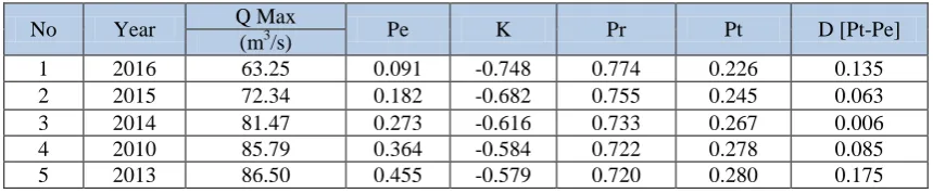
Table 10. Smirnov-Kolmogorov test for the Normal distribution

No Year Q Max Pe K Pr Pt D [Pt-Pe]

(m3/s)

1 2016 63.25 0.091 -0.748 0.774 0.226 0.135

2 2015 72.34 0.182 -0.682 0.755 0.245 0.063

3 2014 81.47 0.273 -0.616 0.733 0.267 0.006

4 2010 85.79 0.364 -0.584 0.722 0.278 0.085

(10)

6 2011 127.85 0.545 -0.279 0.610 0.390 0.155

7 2012 175.29 0.636 0.064 0.474 0.526 0.111

8 2008 202.54 0.727 0.262 0.396 0.604 0.123

9 2009 254.67 0.818 0.640 0.260 0.740 0.078

10 2007 514.42 0.909 2.522 0.006 0.994 0.085

Source: own study

Explanation: Pe = empirical probability; Pt = theoretical probability; D = deviation

Table 11. Smirnov-Kolmogorov test for the Log Normal distribution

No year Q Max Log Q Pe K Pr Pt D [Pt-Pe]

(m3/s)

1 2016 63.25 1.801 0.091 -1.101 0.860 0.140 0.049

2 2015 72.34 1.859 0.182 -0.901 0.814 0.186 0.004

3 2014 81.47 1.911 0.273 -0.723 0.767 0.233 0.040

4 2010 85.79 1.933 0.364 -0.646 0.744 0.256 0.107

5 2013 86.50 1.937 0.455 -0.634 0.739 0.261 0.194

6 2011 127.85 2.107 0.545 -0.051 0.520 0.480 0.066

7 2012 175.29 2.244 0.636 0.419 0.337 0.663 0.026

8 2008 202.54 2.307 0.727 0.635 0.262 0.738 0.011

9 2009 254.67 2.406 0.818 0.976 0.169 0.831 0.013

10 2007 514.42 2.711 0.909 2.025 0.022 0.978 0.069

Source: own study

Table 12. Smirnov-Kolmogorov test for the Log Pearson Type III distribution

No Year Q Max Pe Log Q K Pr Pt D [Pt-Pe]

(m3/s)

1 2016 63.25 0.091 1.801 -1.101 0.885 0.115 0.024

2 2015 72.34 0.182 1.859 -0.901 0.816 0.184 0.002

3 2014 81.47 0.273 1.911 -0.723 0.744 0.256 0.017

4 2010 85.79 0.364 1.933 -0.646 0.712 0.288 0.075

5 2013 86.50 0.455 1.937 -0.634 0.706 0.294 0.161

6 2011 127.85 0.545 2.107 -0.051 0.468 0.532 0.013

7 2012 175.29 0.636 2.244 0.419 0.314 0.686 0.050

8 2008 202.54 0.727 2.307 0.635 0.243 0.757 0.029

9 2009 254.67 0.818 2.406 0.976 0.163 0.837 0.018

10 2007 514.42 0.909 2.711 2.025 0.040 0.960 0.051

Source: own study, Explanation: Pe = empirical probability; Pt = theoretical probability; D = deviation

Table 13. Smirnov-Kolmogorov test for the Gumbel distribution

No Year Q Max P K Yt Tr Pr D [1-Pr-Pe]

(m3/s)

1 2016 63.25 0.091 -0.748 -0.251 1.382 0.723 0.186

2 2015 72.34 0.182 -0.682 -0.188 1.427 0.701 0.117

(11)

4 2010 85.79 0.364 -0.584 -0.096 1.499 0.667 0.031

5 2013 86.50 0.455 -0.579 -0.091 1.503 0.665 0.120

6 2011 127.85 0.545 -0.279 0.194 1.782 0.561 0.107

7 2012 175.29 0.636 0.064 0.520 2.232 0.448 0.084

8 2008 202.54 0.727 0.262 0.708 2.570 0.389 0.116

9 2009 254.67 0.818 0.640 1.067 3.434 0.291 0.109

10 2007 514.42 0.909 2.522 2.854 17.864 0.056 0.035

Source: own study

3.7. Testing of goodness of fit by using the Chi- Square distribution

Test of chi square distribution evaluates the difference between the sample data and the probability distribution.

The formula of chi square is as follow:

(6)

where X2 = chi-square calculated value; Ei = frequency that is hoped regarding to the class division; Oi= frequency

on the same class; N = number of class. The value of Ei can be found with the formula as follow:

(7)

Where, n = number of N = number of class.

Testing of goodness of fit by using chi square distribution test for evaluating the frequency analysis by using the

Normal distribution, the Log Normal distribution, the Log Pearson Type III distribution, and the Gumbel

distribution. The results are presented each on the Table 14, 15, 16, and 17

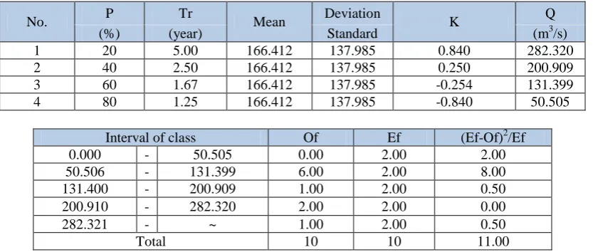
Table 14. Chi-Square test for the Normal distribution

No. P Tr Mean Deviation K Q

(%) (year) Standard (m3/s)

1 20 5.00 166.412 137.985 0.840 282.320

2 40 2.50 166.412 137.985 0.250 200.909

3 60 1.67 166.412 137.985 -0.254 131.399

4 80 1.25 166.412 137.985 -0.840 50.505

Interval of class Of Ef (Ef-Of)2/Ef

0.000 - 50.505 0.00 2.00 2.00

50.506 - 131.399 6.00 2.00 8.00

131.400 - 200.909 1.00 2.00 0.50

200.910 - 282.320 2.00 2.00 0.00

282.321 - ~ 1.00 2.00 0.50

(12)

Chi-square calculated value = 11.00

α (%) = 5%

degree of freedom (g) = 2 = k-h-1 h =2

Chi-square critic = 5.99 non accepted

Source: own study

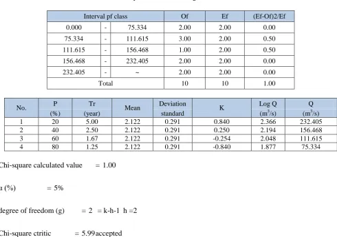
Table 15. Chi-Square test for the Log Normal distribution

Interval pf class Of Ef (Ef-Of)2/Ef

0.000 - 75.334 2.00 2.00 0.00

75.334 - 111.615 3.00 2.00 0.50

111.615 - 156.468 1.00 2.00 0.50

156.468 - 232.405 2.00 2.00 0.00

232.405 - ~ 2.00 2.00 0.00

Total 10 10 1.00

No. P Tr Mean Deviation K Log Q Q

(%) (year) standard (m3/s) (m3/s)

1 20 5.00 2.122 0.291 0.840 2.366 232.405

2 40 2.50 2.122 0.291 0.250 2.194 156.468

3 60 1.67 2.122 0.291 -0.254 2.048 111.615

4 80 1.25 2.122 0.291 -0.840 1.877 75.334

α (%) = 5%

Chi-square ctritic = 5.99 accepted

Table 16. Chi-Square test for the Log Pearson Type III distribution

No. P Mean Deviation Cs K Q

(%) standard Log (m3/s)

1 20 2.122 0.291 0.916 0.787 2.351 224.295

2 40 2.122 0.291 0.916 0.164 2.169 147.695

3 60 2.122 0.291 0.916 -0.391 2.008 101.782

(13)

0.00 - 73.407 2.00 2.00 0.00

73.407 - 101.782 3.00 2.00 0.50

101.782 - 147.695 1.00 2.00 0.50

147.695 - 224.295 2.00 2.00 0.00

224.295 - ~ 2.00 2.00 0.00

Total 10 10 1.00

α (%) = 5%

Chi-square critic = 5.99 accepted

Source: own study

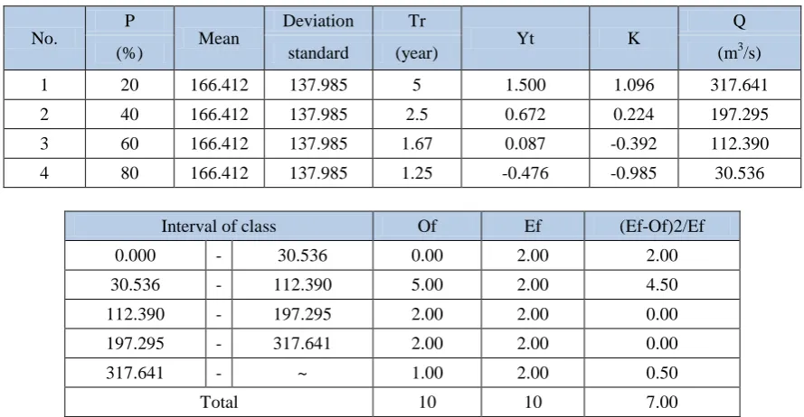
Table 17. Chi-Square test for the Gumbel distribution

No.

P

Mean

Deviation Tr

Yt K

Q

(%) standard (year) (m3/s)

1 20 166.412 137.985 5 1.500 1.096 317.641

2 40 166.412 137.985 2.5 0.672 0.224 197.295

3 60 166.412 137.985 1.67 0.087 -0.392 112.390

4 80 166.412 137.985 1.25 -0.476 -0.985 30.536

0.000 - 30.536 0.00 2.00 2.00

30.536 - 112.390 5.00 2.00 4.50

112.390 - 197.295 2.00 2.00 0.00

197.295 - 317.641 2.00 2.00 0.00

317.641 - ~ 1.00 2.00 0.50

Total 10 10 7.00

α (%) = 5%

Chi-square critic = 5.99 non accepted

(14)

Sn = 0.950

Source: own study

4.

CONCLUSION

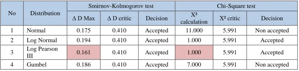
Based on the statistical analysis result as above which includes the Normal distribution, the Log Normal

distribution, the Log Pearson Type III distribution, and the Gumbel distribution, it can be concluded that the rainfall

data from 2007 until 2016 due to the four distributions can be accepted regarding to the Smirnov-Kolmogorof test.

However, based on the chi square test, the Normal distribution and the Gumbel distribution are not accepted. Table

18 presents the recapitulation of test results.

Table 18. The recapitulation of test results for every distribution

No Distribution

Smirnov-Kolmogorov test Chi-Square test

∆ D Max ∆ D critic Decision X²

calculation X² critic Decision

1 Normal 0.175 0.410 Accepted 11.000 5.991 Non accepted

2 Log Normal 0.194 0.410 Accepted 1.000 5.991 Accepted

3 Log Pearson

III 0.161 0.410 Accepted 1.000 5.991 Accepted

4 Gumbel 0.186 0.410 Accepted 7.000 5.991 Non accepted

Source: own study

Based on the result as above, it can be selected the Log Pearson Type III distribution as the suitable distribution for

the Lesti sub-watershed. It is due to the result which indicates that the Log Pearson Type III is accepted for the two

testing of goodness of fit and has the minimum deviation.

REFERENCES

[1] Radevski, I; Gorin, S; Dimitrovska, O; Milevski, I, Apostolovska, B; Taleska, M; and Zlatanoski, V. 2016.

Estimation of maximum annual discharges by frequency analysis with four probability distribution in case of

non-homogeneous time series (Kazani Karst Spring in Republic of Macedonia). Acta Carsalogica, 45(3): 253-262,

Postoina.

[2] Selaman, O.S.; Said, S; and F.J. Putuhena. 2007. Flood frequency analysis for Sarawak using Weibull,

Gringorten and L-Moments formula. Journal-The Institution of Engineers, 68(1): 43-52.

[3] Guru, N. and R. Jha. 2015. Flood frequency analysis for Tel sub-basin of Mahanadi River, India using Weibull,

Gringorten and L-moments formula. International Journal of Innovative Research and Creative Technology, 1(2):

220-223.

[4] US Water Resources Council (USWRC). 1981. Guidennes for determining flood flow frequency. Bulletin No.

(15)

[5] Ahmad, I; Z., Ahmad.; and S.A.,Ahmad. 2012. Flood frequencies to Soan Valley. Pakistan Journal of

Sciences, 64(1): 1-6.

[6] Chow, V.T.; D.R., Maidment; and W. Larry. 1988. Applied hydrology. Mc. Graw Hill Book Company, New

York, USA, pp 380-405.

[7] Kpttegoda, N.T. 1980. Stochastic water resources technology. The Macmillan Press Ltd, pp. 38-46.

[8] Hyun-Han Kwon; Young-Il Moon; and Abedalraszq, F. Khalil. 2007. Nonparametric Monte Carlo simulation

for flood frequency curve derivation: an application to a Korean watershed. Journal of the Amaericam Water

Resources Association, 43(5): Biological Sciences Database, 1316-1328.

[9] Hosking, J.R,M. 1990. L-Moment – analysis and estimation of distribution using linear-combination of

order-statistics. Journal of the Royal Statistical Society SeriesB-Methodological, 52(1): 271-281.

[10]Hosking, J.R.M. and J.R. Wallis. 1993. Some statistics useful in regional frequency analysis. Water Resources

Research, 29(2); 271-0181.

[11]Moon, Y.I. and U. Lall. 1994. Kernel quantile function estimator for flood frequency analysis. Water

Resources research, 30(110; 3096-3100.

[12]Soewarno 1995. Hidrologi aplikasi metode statistik untuk analisa data [Statistical method of hydrological