Abstract— Wind farm collector network design consists primarily in finding a radial configuration to connect a set of wind generators to a substation. Depending on the size of the wind farm, the design of the project, considering the economic criterion, consists of a large combinatorial optimization problem, given the large number of possible configurations to be deployed. Thus, this article proposes a methodology based on a genetic algorithm (GA). The wording adopted in the GA considers the sizing of the collector network in which the investment in the construction and the present value of energy losses are adopted as the objective function in the optimization process. First, the mathematical model to define the objective function is presented, then the encoding of the chromosome is defined and the aptitude encoding function is described, and finally, the results and the more economically viable configuration are presented.
Index Term— wind farm infrastructure; collector network; network configuration; genetic algorithm; network optimization.
1. INTRODUCTION
The strong acceleration in energy consumption observed in recent decades brings the challenge to continue to develop and promote the reduction of environmental impact with an energy matrix still heavily based on fossil fuels. It is in this challenging environment and great difficulty that the opportunity arises for the use of renewable energy, especially including wind power.
The use of wind power to generate electricity on a large scale is achieved by installing several wind turbines on a site, forming a wind power plant, now called a wind farm. This solution proved to be technically and economically feasible [1] and is applied worldwide with the implementation of wind farms connected to the grid driving the growth of this form of energy.
The development of wind power in Brazil in recent years is quite significant, from 237 GWh in 2006 to 5050 GWh in 2012 [2].
Because of this considerable progress, a significant increase in demand is expected for projects of the electric collectors of wind farm systems. The use of optimization techniques in
these projects, helping to increase efficiency and align the sustainability actions, necessitates a new development model.
The wind farm project involves complex studies related to definitions of geographical locations of the wind generators and their specifications, depending on the wind profiles in the region; systemic electrical studies; structural calculations for the construction of bases of the wind turbines; electrical and civil design of the substation and design of the medium-voltage network internal to the wind farm, called the collector network, including its configuration and the interconnection dimensioning; and other factors.
The objective of this paper is to present a methodology for wind farm collector network optimization to obtain the best solution based on deployment and operational costs.
The design of a wind farm collector network primarily defines the best topology of the collector network and its sizing. The definition of the topology of the collector networks is necessarily a large combinatorial optimization problem, given the large number of candidate network configurations. The problem is not simply to be treated; it should resort to iterative methods where the result converges on the best feasible solution.
The collector network design analysis of a wind farm resembles the expansion planning done for power distribution systems. The basic difference is the direction of power flow. This similarity has advantages because designers can use the experiences and solutions already established for use in wind farm collector networks [3].
In this regard, in [4], a conductor optimization algorithm is proposed in radial distribution systems. In [5], genetic algorithms (GAs) to solve large distribution systems are used, to search for the optimum design of electrical cables and the ideal location of substations based on nonlinear mixed integer programming.
Meanwhile, in [6], an evolutionary algorithm for optimal selection of conductor losses based on the reduction of radial distribution systems is proposed. The development of new techniques that enable GAs to set up large networks in a feasible time is shown in [7]. In [8], a comparative study using a conventional optimization method and a method based on a
Duailibe, Paulo R. Monteiro
1;
Soares, Carlos Alberto P.
2; Borges, Thiago T.
3; Schiochet, André F.
41 2 Civil Engineering Graduate Program, Fluminense Federal University, Rua Passo da Pátria, Niterói, Brasil, CEP
24210-240. 3 Department of Electrical Engineering, Fluminense Federal University, Rua Passo da Pátria, 156, Niterói, Brasil, CEP 24210-240. 4 Petróleo Brasileiro S.A., Rua Henrique Valadares, 28, Rio de Janeiro, Brasil, CEP
20231-030.
Methodology for Sizing Wind Farm Collector
Network Infrastructure using a Genetic
Legend
wind generators substation GA in order to minimize losses is presented, maintaining
tension within acceptable limits. The GA showed better results than the conventional method in the tested cases. In [9], a method is proposed for reconfiguring the distribution network to reduce losses and improve reliability. An advanced genetic optimization algorithm is used to deal with the problem of reconfiguration to determine the operating regimes of the keys.
In the wind farm collector network proposed in [3], a GA optimizes the resources for the internal network planning phase of a wind farm, and in [10], a search approach for the best grid project for offshore wind farms uses an improved GA that considers different sections of drivers when designing the radial arrays.
In this paper, we propose a methodology based on the GA to optimize the topology and economic design of wind farm conductors.
2 MATHEMATICALMODELING
The problem for the calculation of a wind farm collector system is mainly to find an ideal radial configuration that connects a set of wind turbines, such that investments in construction and operating costs are minimal, given the pre-defined technical requirements.
While GAs perform a blind search, there is a need for a guide so as to guide them toward the optimum solution. Thus, it is necessary to find a function that guides the GA in pursuit of the objective of the problem. Thus, mathematical modeling is needed to define a function that should reflect the objectives to be achieved in solving the problem.
According to [11], the problems can be treated by considering the optimization of one or more objective functions. In addition, according to the author, the problems can be modeled considering technical and economic constraints, or other factors. According to [12], such a function is the method used by the GA to determine the quality of an individual, thus solving the problem.
According to [13], the objective function of an optimization problem is built from the parameters involved in the problem. It provides a measure of the closeness of the solution in relation to a set of parameters. The goal is to find the optimum point, which is the minimization of this function.
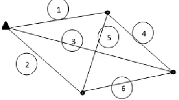
For this treatment, the problem will consider wind turbines and the substation with their geographic locations in order to enable the calculation of distances, where each point is composed of a coordinate (x, y). Thus, a hypothetical situation of a wind farm is shown in Figure 1 with a way to interconnect the turbines among several possible modes.
Fig. 1. Position of wind generators and substation of a fictitious wind farm with a feasible configuration of the collector network.
To find the best radial topology that connects all the wind turbines to the substation so as to minimize the implementation costs of the sum of the present value of energy losses in a planning horizon, the following formulation is employed:
Min f(r), such that rCr (1)
where r is a collector network configuration park and Cr is the set of all feasible related radial configurations. Feasible configurations are considered to be those in which the current flow in the paths is compatible with the maximum current carrying capacity of the conductors and meet the criteria of established voltage drop and the economic sizing of the cable.
To meet the proposed objective function f(r), formulation (1) is defined as:
f(r) = f(implementation) + f(losses) (2)
where
f(implementation) = nc $cg+ nc $cs+
(3) and
f(losses) = KpPe$MWh (4)
Then, according to expression (2),
f(r) = nc $cg+ nc $cs + + KpPe$MWh
(5)
where:
nc number of circuits
$cg cost per output cubicle of each generator
$cs cost per cubicle of each circuit connection substation li length of stretch i (km)
0
2
3 $ci cost per km of the cable to be installed on stretch i
nt number of stretches in the collector network
$Ici cost per km of the cable installation to be cable in stretch i
kp loss factor in wind of the daily and seasonal variations
function
Pe energy losses in the collector network (MWh/year)
$MWhcost of energy (R$/MWh)
i correction rate per year
A number of years in the planning horizon of the project
The f(r) function reveals the collector network deployment costs and their respective circuit receiving panels in the substation and the panels of each generator, as well as the operating costs.
Thus, minimizing the function f(r) means finding the most economical solution to the collector network of the wind farm, not only for the implementation costs but also the associated operating costs of the reduction of energy losses over the project horizon.
It is relevant to note that in calculating the implementation of the collector network, there are two fixed costs per circuit: the cost of the cubicles at both ends of the circuit and the cost related to the deployment of each portion of the collector network. The first cost for each section of the network, referred to the conductor cost itself, is selected from a family of candidate conductors eligible by supportability, impedances, and cost per kilometer. The second refers to the construction cost per kilometer depending on the type of installation from possible facilities established.
The present value of the loss is calculated from the total first-year energy losses by applying the annual rate of correction to the loss of the following years to the horizon of the project. This calculation assumes the wind turbines operate within their limits. It is available in the formula by the factor kp, losses representing the daily and seasonal variations of wind in the project area.
3 PROPOSEDSOLUTION
To solve the problem, a methodology is proposed based on the GA, with a chromosome coding edge using binary numbers.
Genetic crossover and mutation special operators are used, and the stop is given when the maximum generation number is reached or when a population does not improve in successive generations. To preserve the characteristics of the best individual solution in the next generation, the proposed GA also uses elitism. In the end, the algorithm provides the topology to be built and the costs.
This section is divided into four parts: the first two show the encoding and decoding proposal, followed by the approach that makes up the special functions of the GA; finally, the fitness function is described.
3.1 Coding Scheme
Modeling by graphs of the topology of a collector network
uses the example of a small dummy wind farm containing a substation and three wind turbines, arranged as shown in Figure 2. The substation is represented by solid triangle, the windmills are solid black circles, and edges are numbered 1 to 6. Figure 3 shows a feasible configuration collector network for this example.
Fig. 2. Largest possible number of edges of a fictitious wind farm.
To establish a coding edge with binary numbers for the genetic model example of the fictitious wind farm, where there is only a single substation node and three generator nodes, the individual encoding of the network to the topology of Figure 3 will have the chromosome presented in Figure 4.
Fig. 3. Feasible topology for the system example.
2 2 2 2 2 2 Maximum
1 1 0 0 0 1 Chromosome
1 2 3 4 5 6 Edge
Fig. 4. Codification of the collector network topology in Figure 3.
In Figure 4, the chromosome that encodes the collector system is highlighted by a gray background and has a length equal to the maximum possible number of edges. Above each gene are their maximum limits, and in the bottom line are the identifiers of the edges associated with each gene. The ceiling of each chromosome gene corresponds to the binary numbers (0 and 1), where 0 means off-edge and 1 means edge-connected.
By adopting this definition, the GA considers that the edge encoded with 0 “does not exist” in this topology and the edge with 1 “exists,” and the network topology is drawn accordingly.
showing the adhesion of chromosome encoding for the topology of Figure 3. It is important to note that in this example the chromosome size is 6, equal to the number of possible edges for this example as seen in Figure 2.
3.2 Decoding
Decoding adopts the premise that all the edges are turned off or are not (code 0). Taking as an example the decoding of the individual Figure 4, the procedure is to go to each chromosome, in any order, and where the gene number 1 is found, a new edge is created. Thus, taking the second element of Figure 4, A (2) = 1, associated with edge 2 as the gene is encoded with the number 1, this edge is created connecting the substation node 0 to generator node 2. Thus, all edges with gene number 1 are created, and edges with gene number 0 are disregarded.
As can be seen, decoding is direct. The procedure is repeated for each gene, resulting in the creation of the three edges represented in Figure 3.
3.3 Special features of the proposed GA
In the proposed algorithm, special features were created in the generation of the initial population, crossover operators, and mutation, modifying them to create only radial and connected individuals. For the generation of the initial population, a heuristic was implemented to create only radial and related individuals. Similarly, when there is crossover and mutation, new individuals are tested for connectivity and radial configuration, thus ensuring that all individuals of the new population are radial and connected.
3.4 Methodology for calculating the fitness function
The fitness function determines the value of each individual in the population. This function measures how close a particular solution (individual) is to the desired solution. The algorithm performs a blind search, guided exclusively by this function.
The objective function defined in equation (5) covers the objectives set out in this work. Fitness includes the objective function and sizes and calculates the components and network parameters necessary for the evaluation of the population.
Initially it makes an economic calculation of the cable to set the current ranges of the family of competitor cables outside the GA. The upper and lower limits of current in amperes for the economic range of a given conductor section are calculated by the following equations [14]:
√
(6)
√
(7)
where:
CI is the cost of cable length installation, whose section is being considered, expressed as a unit of currency ($)
R It is the a.c. resistance per unit length of the cable section being considered, expressed in ohms per meter (Ω/m)
Cl1 is the cost of installing the next lower cable nominal section, expressed in currency unit ($)
R1 It is the a.c. resistance per unit length of the next lower cable nominal section, expressed in ohms per meter (Ω/m) CI2 is the cost of installing the next larger cable of nominal section, expressed in currency unit ($)
R2 It is the a.c. resistance per unit length of the next larger nominal cable section, expressed in ohms per meter (Ω/m)
Thus, with the knowledge of the currents in the paths, the GA sets the optimum cable for each section on the basis of the current ranges established in the economic calculation of the driver. Table 1 shows the fitness calculation methodology that evaluates individuals.
TABLEI
METHODOLOGYOFFITNESSCALCULATION
STEP DESCRIPTION OBJECTIVE
1 Decoding the individual --- 2 Adopt all branches with
the largest cable
---
3 Turning load flow Calculate current
in the branches 4 Size cables for the criteria
of current conduction capacity, optimized cable, and voltage drop
Set the optimum cable in each branch
5 Turning load flow Calculate the loss
of active power 6 Apply the objective
function
Calculate the investment cost and further operational costs. Ranked by population
4 SYSTEM TEST
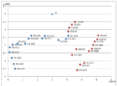
In order to validate the proposed model, an already tested and solved collector network was chosen as an example for comparison with the proposed model. This example was presented in [3]; the system comprises two wind farms, each consisting of 15 wind generators of 2 MW rated power.
The wind farm characteristics used for testing are as follows:
• Voltage of the collector network: 34.5 kV • Substation capacity: 80 MVA
• Cost per cubicle feeder output: R$ 100,000.00 • Typical loss factor for the studied region: 0.21 • Energy cost: R$200.00/MWh
• Annual correction rate: 11% • Planning horizon: 20 years
TABLEII
INPUTDATAASSOCIATEDWITHFARM1
Identification x (km) y (km)
SE 3.0 4.0
01-G01 1.578 2.621
01-G02 0.315 2.037
01-G03 0.477 0.498
01-G04 1.165 2.098
01-G05 2.311 2.431
01-G06 1.401 2.426
01-G07 3.937 2.404
01-G08 3.413 2.337
01-G09 0.387 0.809
01-G10 0.254 1.195
01-G11 0.11 1.863
01-G12 0.099 1.56
01-G13 0.648 2.12
01-G14 4.086 2.608
01-G15 2.497 2.599
TABLEIII
INPUTDATAASSOCIATEDWITHFARM2
Identification x (km) y (km)
02-G01 5.171 0.866
02-G02 6.113 2.626
02-G03 4.348 1.381
02-G04 5.777 2.011
02-G05 5.879 2.242
02-G06 4.533 3.496
02-G07 4.33 3.322
02-G08 5.485 1.629
02-G09 5.688 1.782
02-G10 4.634 1.748
02-G11 4.085 2.89
02-G12 4.151 3.131
02-G13 6.054 2.376
02-G14 4.689 0.412
02-G15 4.887 0.759
Fig. 5. Spatial arrangement of farms 1 and 2 used for validation.
TABLEIV
INPUTDATAASSOCIATEDWITHCABLES/STRUCTURES
The results of the example that will be used to test the proposed model were obtained from [3] and are presented in Table V and in Figure 6.
TABLEV
COSTSOFTHEBESTFEASIBLESOLUTIONFORWINDFARMS1AND
2
Cable R
(/km) X (/km)
R$/km Capacity
(A)
C095 0.4301 0.142 78,090.00 177
C120 0.3403 0.136 83,310.00 194
C150 0.2773 0.134 89,340.00 216
C185 0.2212 0.129 94,200.00 244
C240 0.1693 0.122 100,710.00 283
C300 0.1362 0.119 113,310.00 319
C400 0.1071 0.115 130,110.00 364
Wind Farm
Loss (R$)
Investment (R$)
Total (R$) 1 449,418.44 1,095,415.73 1,544,834.17
Fig. 6. Spatial arrangement with the best feasible solution for wind farms 1 and 2.
4.1 Proposed model validation
In order to validate the proposed model, it was applied to the same wind farm presented in this section. For method comparison, the same input data were used.
4.1.1 Results for the proposed model for wind farm 1
The application of the proposed model to wind farm 1 resulted in the following alternative for the collector network. The costs are presented in Table VI.
TABLEVI.
RESULTSFORWINDFARM1
Loss (R$)
Investment (R$)
Total (R$)
449,418.44 1,095,415.73 1,544,834.17
Comparing costs of wind farm 1 in Table 5 obtained from [3] with the costs of Table VI reveals that the same results were obtained for wind farm 1, validating then proposed model. Similarly, the topology obtained for wind farm 1 is also the same of the one presented in Figure 6.
4.1.2 Results for the proposed model for wind farm 2
The same comparison was carried out for wind farm 2. The result is presented in Table VII.
TABLEVII.
RESULTSFORWINDFARM2
Loss (R$)
Investment (R$)
Total (R$)
430,930.46 1,189,146.46 1,620,076.92
The best alternative for wind farm 2 came to a total cost of R$ 1,620,076.92, lower than the one presented in Table 5 for wind farm 2 obtained from [3]. It can also be observed that this solution has lower costs when the losses and investment
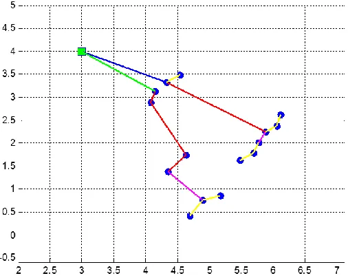
reductions are separately evaluated. The topology of this alternative is presented in Figure 7 and is different from the one found in the example.
Fig. 7. Arrangement of the best feasible solution for wind farm 2 per the proposed model.
In Figure 7, the substation is represented by the square, whereas the wind generators are represented by circles. The edges in yellow represent the 95 mm² cable, in magenta the 120 mm² cable, in cyan the 185 mm² cable, in red the 240 mm² cable, in green the 300 m² cable, and in blue the 400 mm² cable. The coordinates are in km.
When comparing the solutions presented by the two models, it is observed that the solution of the model proposed shows a topology more balanced in the distribution of aerogenerators per circuit. While the topology of the test example shows a circuit with six aerogenerators and other circuit with nine; in the topology of the proposed method, a circuit has seven aerogenerators and the other circuit has eight, better dividing the loads in the circuits. Furthermore, the GA implementation of proposed method reduces the search space of solutions, since the cables are selected within the fitness function The result achieved is due to the attributes of the proposed method and demonstrates its effectiveness.
5 CONCLUSION
This study proposes and validates a methodology based on wind generators with the optimal cable calculation for application in wind farm collectors networks, using as an optimization criterion the investment and operational costs. There was no violation of the supportability of the cables, and the voltage drop requirements were met for the elected solutions.
REFERENCES
[1] MORA, J. C. Optimización global de parques eólicos mediante
algoritmos evolutivos. Tesis Doctoral, Universidad de Sevilla, 2008.
[2] EMPRESA DE PESQUISA ENERGÉTICA. Balanço energético
nacional 2013: Ano base 2012. Rio de Janeiro: EPE, 2013.
[3] BRAZ, Helon D.M. et al. Planejamento da rede coletora de um parque
de geração eólica usando algoritmos genéticos. Simpósio Brasileiro de Sistemas Elétricos, UFCG, Brasil, Julho, 17-19, pp. 1-6, 2006.
[4] TRAM, H. N.; WALL, D. L. Optimal conductor selection in planning
radial distribution systems. Power Systems, IEEE Transactions on, v. 3, n. 1, p. 200-206, 1988.
[5] RAMIREZ-ROSADO, Ignacio J.; BERNAL-AGUSTIN, Jose L.
Genetic algorithms applied to the design of large power distribution systems. Power Systems, IEEE Transactions on, v. 13, n. 2, p. 696-703, 1998.
[6] RAO, R. Srinivasa. Optimal conductor selection for loss reduction in radial distribution systems using differential evolution. International Journal of Engineering Science and Technology, v. 2, n. 7, p. 2829-2838, 2010.
[7] BRAZ, H. D. de M. Configuração de Sistemas de Distribuição usando
um Algoritmo Genético Sequencial. Tese de Doutorado: Universidade Federal de Campina Grande, 2010.
[8] THENEPALLE, Muralimohan. A comparative study on optimal
conductor selection for radial distribution network using conventional and genetic algorithm approach. International Journal of Computer Applications (IJCA), v. 17, n. 2, p. 6-13, 2011.
[9] DUAN, Dong-Li et al. Reconfiguration of distribution network for loss
reduction and reliability improvement based on an enhanced genetic algorithm. International Journal of Electrical Power & Energy Systems, v. 64, p. 88-95, 2015.
[10] GONZÁLEZ-LONGATT, Francisco M. et al. Optimal electric network
design for a large offshore wind farm based on a modified genetic algorithm approach. Systems Journal, IEEE, v. 6, n. 1, p. 164-172, 2012.
[11] KAGAN, N.; BARIONI DE OLIVEIRA, C. C.; SCHMIDT H. P.; KAGAN H. Métodos de otimização aplicados a sistemas elétricos de potência. Blucher, 2009.
[12] LINDEN, Ricardo. Algoritmos Genéticos: Uma Importante Ferramenta
da Inteligencia Computacional. Editora Brasport. Rio de Janeiro, 2006.
[13] MIRANDA, Marcio Nunes de. Algoritmos Genéticos: Fundamentos e
Aplicações. 2007
[14] ASSOCIAÇÃO BRASILEIRA DE NORMAS TÉCNICAS - ABNT
NBR-15920, Cabos elétricos — Cálculo da corrente nominal —