O R I G I N A L A R T I C L E
Open Access
Evaluating search and matching models
using experimental data
Jeremy Lise
1,2, Shannon Seitz
3and Jeffrey Smith
4,5,6**Correspondence: [email protected] 4Department of Economics, University of Michigan, 611 Tappan Street, Ann Arbor, MI 48109-1220, USA
5NBER, Cambridge, USA Full list of author information is available at the end of the article
Abstract
This paper introduces an innovative test of search and matching models using the exogenous variation available in experimental data. We take an off-the-shelf search model and calibrate it to data on thecontrolgroup from a randomized social
experiment. We then simulate aprogramgroup from a randomized experiment within the model. As a measure of the performance of the model, we compare the outcomes of the program groups from the model and from the randomized experiment. We illustrate our methodology using the Canadian Self-Sufficiency Project (SSP), a social experiment providing a time-limited earnings supplement for Income Assistance recipients who obtain full-time employment within a 12-month period. We find two features of the model are consistent with the experimental results: endogenous search intensity andexogenousjob destruction. We find mixed evidence in support of the assumption of fixed hours of labor supply. Finally, we find aconstantjob destruction rate is not consistent with the experimental data in this context.
JEL Classification: J2; I38; J6
Keywords: Policy experiments; Search and matching; Self-sufficiency project; Social experiments
1 Introduction
Search and matching models in the spirit of McCall (1970) or Diamond (1982), Mortensen (1982) and Pissarides (1985) (DMP) are an important tool for the evaluation of new or existing labor market policies.1The policy experiments conducted within such models allow consideration of the potential effects of policy reforms that have yet to be imple-mented in reality as well as the general equilibrium effects of large-scale reforms or of small-scale reforms that may be implemented on a large-scale in the future. They also allow what one might call theoretically structured mediation (or decomposition) analy-sis, wherein the model aids in empirically sorting out the causal channels underlying the “black box” impact estimates that emerge from design-based studies. Despite the impor-tance of this policy evaluation tool, it is difficult to put a high degree of confidence in the quantitative results of such exercises, as it is often difficult to judge how well the model captures the responses of individuals to changes in government policy.2
In general, the literature evaluates the performance of structural economic models, such as those in the search and matching literature, in two ways. The most common way con-siders the in-sample fit of the model relative to the moments used in the calibration or
estimation. In many cases, the ability of the model to match moments not included in the calibration or estimation process, but drawn from the same empirical context, is also used as a test of the model.3This sort of test represents an important starting point to ensure the benchmark model can replicate behavior observed in the data used to calibrate or estimate it. However, such tests provide no direct evidence on how reliable the model pre-dictions are under changes to the policy environment. The second way to gauge a model’s performance is out-of-sample tests, where the fit to other time periods (or other empirical contexts more generally) is used as a test of the model. This is a more demanding mea-sure of performance, as the model’s predictions are compared to an environment outside of the calibration or estimation process. However, because many features of the economy vary over time, it is difficult to gauge the extent to which the comparison between out-of-sample statistics and the model predictions are contaminated by changes in factors not captured by the model.4
The contribution of our paper is twofold. First, we introduce a new and convincing test of the quantitative performance of search and matching models. The new test that we consider exploits the wealth of information available through social experiments (and readily generalizes to the broader set of compelling non-experimental impact analyses). In social experiments, small subsets of the population are randomly assigned to program and control groups; the program group is subjected to a potential policy reform, and the difference in outcomes between the groups provides an estimate of the mean impact of the policy.5Social experiments provide compelling causal estimates of how individuals within the experiment respond to the incentives introduced by the policy reform. It is in this sense that social experiments provide an excellent opportunity to determine whether a particular model, once calibrated or estimated, can accurately predict the effects of policy changes.6
The basic idea behind our approach is the following: First, we calibrate our model of interest to match the behavior of the control group from a randomized experiment. Sec-ond, we introduce the policy of interest in the model and use the calibrated model to simulate a program group. Third, we compare the outcomes of the model program group with the outcomes of the experimental program group. The model is asked to match the outcomes of the program group without relying on the exogenous variation introduced within the experiment. Further, as in the model, the only change in the economic envi-ronment that is introduced in the experiment is the policy change of interest. Therefore, we obtain a test of the model uncontaminated by changes in other factors that could blur the comparison between the model and the data. In this respect, the social experiment provides a very rigorous test of the model.7
model is augmented to incorporate the main features of the SSP. In particular, the model allows for time limits in determining eligibility for receipt of the supplement, consistent with the one-year time limit in the experiment, allows individuals to receive the earnings supplement for up to three years while employed, and allows the earnings supplement to depend on the earnings received by eligible recipients. The time limitations for entry to and exit from the Canadian unemployment insurance program (called Employment Insurance or EI) and the interactions between IA, the unemployment program, and the labor market are also incorporated in the model.
The main margin through which the SSP is designed to affect behavior is via increased job search effort by welfare recipients resulting from the time limitations and the financial incentives introduced by the program. Therefore, as in Pissarides (2000, Ch.5), we also introduce endogenous search intensity in the model. Because of the policy focus on search effort we do not include a reservation wage channel in the model. Our paper focuses on testing the partial equilibrium implications of the model, as the SSP is a small-scale experiment that is unlikely to have general equilibrium implications for the labor market. After constructing the model, we calibrate the model in the absence of the program using publicly available, non-experimental data on single mothers and data on the exper-imental control group. The SSP was implemented separately in two provinces, New Brunswick and British Columbia, and we calibrate and test the model separately for each province. The parameters calibrated in the first stage include the discount fac-tor, search friction parameters, and exogenous job separation rates: parameters that are, in theory, invariant to changes in the Income Assistance program. We then simu-late the SSP experiment within our calibrated model and compare the model outcomes for the simulated control group, the simulated program group, and the difference between them (i.e., the simulated experimental impact) to those in the experimental data.
Our tests focus on three features of the model: search intensity, job destruction, and earnings. First, we consider how well the model specification for search intensity matches the experimental data. The parameters governing the choice of search intensity cannot be directly identified in the data and are therefore the margin that we have the least confidence in. We test the search intensity features of the model by comparing the exit rates from IA for the control and program groups in the model to those in the data. In British Columbia, we find that the impacts of the SSP on the IA-to-work transition rates during the 53 months following random assignment in the model are not statistically dif-ferent from those in the experimental data. We are also able to match the delayed-exit effects of a second randomized experiment in British Columbia that offered SSP to new Income Assistance recipients. Along these dimensions, our model test provides strong support for the framework. In contrast, the model predicts a significantly (and substan-tially) higher transition rate from IA to employment with the introduction of the SSP in New Brunswick. The elasticity of search costs with respect to search effort in New Brunswick must be much higher than that in British Columbia to match the experimental impact of the SSP.
program and control groups, even when individuals in the program group stop receiving supplement payments. However, the assumption of a constant job destruction rate is not consistent with the experimental data, as the employment exit hazard rate clearly falls with tenure.
We also assess the effects of the policy change on earnings. In partial equilibrium, we expect no change in earnings, conditional on tenure, due to the small number of individ-uals affected by the policy change in the experiment. For British Columbia, this appears consistent with the data as the earnings-tenure profiles for the employed in the program group do not statistically differ from those for the employed in the control group.9 How-ever, although the earnings-tenure profiles for the employed in the program and control groups are the same, a closer examination of the data indicates that hours are higher in both provinces for those individuals eligible for the SSP, consistent with the program’s focus on full-time work.
In the final component of our analysis, we switch from using the experimental pro-gram group data to test the model to using it to help calibrate the model. This switch embodies in our context the very general tradeoff between using additional restrictions for testing versus using them for calibration or estimation. For example, in a common effects linear instrumental variables context, a researcher with two candidate instrumen-tal variables must choose between using both for estimation, or using one to test the exogeneity of the other. A natural approach within our framework starts with using the experimental variation to test the model and then switches to using it for estimation or calibration once a satisfactory model is found. In the SSP context, using the experimental program group in the calibration changes the results in New Brunswick but not in British Columbia.
We organize the remainder of the paper as follows: Section 2 presents a prototypical matching model with endogenous search intensity. Section 3 outlines our methodol-ogy for testing the model and presents data on the social experiment used to test the model. A comparison of the model experiment and social experiment, including formal model tests, is presented in Section 4, along with sensitivity analysis and the analysis that uses the experimental variation for calibration rather than for testing. Section 5 concludes.
2 The model
social experiment we use to test the model affects only a small number of individu-als and as such is not expected to have any effects on the distribution of wages in the economy.
Key features of typical unemployment insurance and Income Assistance programs are incorporated in the model as follows. First, individuals face time limitations regarding entry to and exit from the unemployment system. Individuals who enter employment from Income Assistance or who have exhausted their unemployment benefits become eligible to receive unemployment benefits afterI months of employment. The number of benefit months subsequently increases by one month for each additional month of employment, from a minimum ofumonths up to a maximum ofu¯months. Workers who enter employment with unused benefits retain their unused benefit months and accu-mulate additional months with each month worked. Second, individuals who exhaust their unemployment benefits and do not secure a job are assumed to transit directly to Income Assistance. Finally, it is assumed that individuals can remain on Income Assis-tance indefinitely or transit to employment if they contact a firm with a vacancy; Income Assistance recipients cannot transit directly from IA to unemployment. In the following sections, we describe the problems faced by individuals in each labor force state in the model.
2.1 IA Recipients
IA recipients receive benefits (ba) and pay search costsca[p(0)z] every month they remain on IA, wherezis the elasticity of search costs with respect to search effort,cais a parame-ter capturing the disutility of search effort, andp(i)is optimal search effort for individuals withimonths of unemployment benefits remaining. The cost of search depends directly on the intensity with which individuals search within the model. In particular, for values ofz>1, the marginal cost of search increases as search effort increases. If IA recipients contact a firm with a vacancy, they transit to employment. Otherwise, they remain on IA in the next period. The value function for an IA recipient is
VA=max p(0)
ba−ca[p(0)z]+β
m(0)VE(1, 0)+(1−m(0))VA
,
where m(0) is the match rate for IA recipients, β is the discount factor, VE(1, 0) is the value of the first period of employment, andVA is the value of being on Income Assistance. The only reason IA recipients are not employed is because an employment opportunity is not available and the only way an IA recipient can increase the likelihood of finding a job is through increased search effort. As we will see below the match rate m(0)is determined in part by search effortp(0).12
2.2 Unemployed individuals
indi-viduals can either transit to employment, if a job opportunity is available, or transit to IA. The value function for unemployed individuals withimonths of benefits remaining is
VU(i)= ⎧ ⎪ ⎪ ⎪ ⎨ ⎪ ⎪ ⎪ ⎩
maxp(i)bu−cu[p(i)z]
+βm(i)VE(1,i−1)+(1−m(i))VU(i−1) 1<i≤ ¯u, maxp(i)bu−cu[p(i)z]
+βm(1)VE(1, 0)+(1−m(1))VA i=1.
2.3 Workers
The value of employment for a worker depends on her job tenure t and unemploy-ment eligibility status i, wherei ∈ {0, 1,. . .,u,. . .,u¯}. As noted above, the number of months an individual with no benefits must work to qualify for unemployment is I. For every period an individual works beyond the qualifying period I, months of eli-gibility i increases by 1. The maximum number of benefit months an individual can accumulate is denotedu¯. If the individual were not working she would therefore be unem-ployed with i periods of benefits remaining. With probabilityδ, jobs are exogenously destroyed in the subsequent month, in which case workers transit to Income Assistance if they have not yet qualified for unemployment benefits (i = 0) and transit to unem-ployment otherwise. With probability (1 − δ) workers remain employed in the next month.
It is assumed that individuals who return to work before their unemployment benefits expire retain their remaining unemployment benefit eligibility. Finally, workers experi-ence on-the-job wage growth for a maximum ofTmonths, after which the wage remains constant, where it is assumedT >u¯. The value function for a worker with outside option iand with job tenuretis:
VE(t,i)= ⎧ ⎪ ⎪ ⎪ ⎪ ⎪ ⎪ ⎪ ⎪ ⎪ ⎪ ⎪ ⎪ ⎪ ⎪ ⎪ ⎨ ⎪ ⎪ ⎪ ⎪ ⎪ ⎪ ⎪ ⎪ ⎪ ⎪ ⎪ ⎪ ⎪ ⎪ ⎪ ⎩
w(t, 0)+β(1−δ)VE(t+1, 0)+δVA ift<Iandi=0, w(t, 0)+β(1−δ)VEt+1,u+δVUu ift=Iandi=0, w(t,i)+β(1−δ)VE(t+1,i)+δVU(i) if 0<i<u¯
andt<I, w(t,i)+β(1−δ)VE(t+1,i+1)+δVU(i+1) if 0<i<u¯
andI≤t<T, w(t,u¯)+β(1−δ)VE(t+1,u¯)+δVU(u¯) ifi= ¯u
andI≤t<T, w(T,u¯)+β(1−δ)VE(T,u¯)+δVU(u¯) ift≥T,
wherew(t,i)is the wage for a person with tenuretwho has unemployment eligibilityi.
2.4 Search technology
We assume there is no on-the-job search in the economy. The probability that a jobless individual receives a job offer depends on the probability the worker contacts a firm and the probability a firm has a vacancy. It is assumed that every firm employs at most one worker.
2.4.1 Workers
assumed that firms randomly draw workers from the applicant pool if there is more than one applicant.13The probability a worker is offered a job is:
1−e−λ λ .
The conditional re-employment probabilities for unemployed workers and workers on Income Assistance can then be expressed as the product of the above components, multiplied by the worker’s search effort
m(i)= p(i)V λF
1−e−λ,
where
λ= 1 F
u¯
i=1
p(i)U(i)+p(0)A
,
U(i)is the number of unemployed workers withimonths of unemployment insurance benefits remaining,Ais the number of workers on IA, andp(0)andp(i)denote the con-tact probabilities for IA recipients and unemployed individuals withiperiods of UI receipt remaining, respectively.14The contact probabilities are choice variables for the workers within the model and can be interpreted as search effort. Workers determine the optimal level of search effort by equating the marginal benefit from an increase in search effort with its marginal cost.15The optimal level of search effort, for each labor market state and program eligibility combination, is the solution to the following:
p(0) = β
m(0) caz
VE(1, 0)−VA 1
z ,
p(1) = β
m(1) cuz
VE(1, 0)−VA 1
z ,i=1,
p(i) = β
m(i) cuz
VE(1,i−1)−VU(i−1) 1
z
, 1<i≤ ¯u.
The model presented above is a well-known model of the labor market. It contains features common to many unemployment and welfare programs and is a model that is straightforward to extend to study many policy reforms. In the next section, we evaluate the performance of the above aspects of the model using experimental data from the SSP.
3 Testing the model with experimental data
In this section, we describe a way to use social experiments as a test of the predictive power of the model. The social experiment we consider here is the Canadian Self-Sufficiency Project. The Self-Self-Sufficiency Project provides an ideal application for this paper, as the policy implemented in the experiment is relatively straightforward to intro-duce in the model and no additional parameters need to be calibrated. We start by providing some details on the SSP and then outline our approach for conducting a partial equilibrium policy evaluation of the Self-Sufficiency Project.16
and control groups by random assignment.19Individuals assigned to the program group were informed that they were to receive an earnings supplement if they found a full-time (30 hours per week) job within one year and left Income Assistance. The supplement received by members of the program group depends on their labor market earnings.20In particular, the supplement payment equals one-half of the difference between the earn-ings of the recipient and a benchmark earnearn-ings level, set at $37,000 in British Columbia and at $30,000 in New Brunswick for those earning less than the benchmark earnings level. Once individuals start receiving the supplement, they continue to do so for up to three years, as long as they remain employed full-time. Individuals in the program group who were not able to secure full-time employment within the twelve months following random assignment were not eligible to receive the supplement. Individuals in the control group were never eligible for the supplement.
The data contain information on 5,685 recipients in the main study: 2,827 control group members and 2,858 program group members.21From the full sample, 4,371 single moth-ers provided information for the 18, 36, and 54 month follow-up surveys. We eliminate a further 1,025 observations for those individuals already employed at random assignment. The remaining sample contains 3,346 respondents, of whom 1,671 are members of the control group and 1,675 are members of the program group.22 This final sample is the one we use for our analysis.
The process we undertake to evaluate the model (and our calibration of it) involves the following three stages:
1. Calibrate the model to the populations targeted by the SSP social experiment and to the control group in the social experiment in each province. This represents the model control groups.
2. Introduce the Self-Sufficiency Project in the model as an experiment. Simulate the behavioral effects of the program in partial equilibrium for each province. This represents ourmodel program groups.
3. Compare the levels and impacts predicted by the model to those observed in the data. This exercise provides evidence on how well our model and simulated experiment are able to replicate the impacts generated by the actual experiment. It is important to emphasize that the partial equilibrium version of the model is the appropriate comparison to the experiment because the experiment only affected a small subset of the economy and as such is not expected to have equilibrium impacts, as compared to a change in policy affecting all IA recipients.
Each step will be discussed in detail below.
3.1 Calibration of the model control group
directly to this literature. Second, some of the key parameters that were calibrated would not have been identified non-parametrically given the data available in the SSP context.24 More broadly, for the most part we are using the same information to calibrate the model that we would have used had we estimated the model. So the parameter values from an estimation exercise would likely not differ substantially from those reported here.
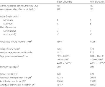
The parameters for the partial equilibrium version of the model include monthly Income Assistance and unemployment benefits (baandbu, respectively), the wage pro-file, the size of the labor force (L), the vacancy rate (V/F), the job separation rate (δ), the discount factor (β), and the search friction parameters (ca, cu,z). The values used for these parameters are all reported in Table 1. Monthly Income Assistance benefits (ba) for single mothers are based on the average IA benefits for a single parent with one child during the 1990s, as reported in the National Council of Welfare Reports (2002). Over this period the average monthly Income Assistance benefit in British Columbia was $927 and in New Brunswick was $737. Unemployment insurance benefits (bu) are set at 55 percent of average earnings. In both provinces, the earnings sample is limited to single mothers without completed post-secondary education, as we are attempting to isolate that segment of the labor market most similar to individuals receiving Income Assistance.25The earnings data are based on the usual hourly wage, as reported in the monthly Labour Force Survey (1997-2000), assuming a 37.5 hour work week.26,27 We
Table 1Moments and parameters for single mothers without completed postsecondary education
British Columbia New Brunswick
Income Assistance benefits, monthly(ba)1 927 737
Unemployment benefits, monthly(bu)2 952 695
UI qualifying months3
Minimum 4 3
Maximum 9 8
UI benefit months
Minimum (u) 5 7
Maximum (u¯) 10 12
Average job tenure, months(1/δ)4 46.68 47.28
Average hourly wage4 10.65 7.78
Average wage, tenure>48 months 11.12 8.22
Wage growth equationw(t)= 7.89+0.0891t 6.04+0.0418t −0.000378t2 −0.0000736t2
+6.10×10⁻⁷t3 +5.51×10⁻⁸t3
Minimum wage(w)5 5.50 5.00
Vacancy rate(V/F)6 3.20 3.20
Exogenous job separation rate(δ)7 0.0214 0.0211
Monthly discount factor(β)8 0.9835 0.9835
Elasticity of search costs w.r.t effort(z)9 1.8457 1.8457
use data from the Labour Force Survey, as opposed to experimental data, as there is not enough wage data (in particular at jobs of long durations) available in the SSP to esti-mate the full wage distribution by tenure. We estiesti-mate a regression with the wage as the dependent variable and a cubic in tenure as the independent variables. We gener-ate predicted values from the regression, for tenures of 1 to 48 months, and multiply the predicted values by 37.5 to obtain a full-time earnings value for each level of tenure. Full-time earnings for those with tenure greater than 48 months are set equal to full-time earnings for workers with tenure equal to 48 months. Earnings, IA benefits and unemployment benefits are all converted to 1992 dollars using the all-goods CPI.28The resulting monthly unemployment benefits level is $952 in British Columbia and $695 in New Brunswick.
The model is homogeneous of degree zero inLandF; we can therefore normalize the size of the labor force to 100 without loss of generality. The number of firms in the econ-omy will be estimated in the baseline model and is identified using the observed vacancy rate in the economy. The following relation determinesVendogenously as a function of FandE:
F=E+V.
In order to estimateF,we use the additional relationship betweenFandV given by the vacancy rate (v)
V F =v.
The vacancy rate of 3.20 % is taken from Galarneau et al. (2001) and is based on the aver-age for the retail trade and consumer services and labor-intensive tertiary manufacturing sectors, both of which have average incomes similar to our sample. Therefore, using the above equations, and for a given value ofE,
F= E
(1−0.032).
The job separation rate in the model (δ) is constant and can be directly estimated by the average job tenure for single mothers with no completed post-secondary education in the monthly Labour Force Survey (1990-2000). Job tenure is only reported for individuals cur-rently employed in the data: we do not have direct information on separations. However, average job tenure is observed and in the model is equal to
∞
t=1tE(t)
E =
E(1)∞t=1t(1−δ)t−1 E(1)∞t=1(1−δ)t−1 =
1 δ.
Average job tenure in the Labour Force Survey (LFS 1990–2000) implies a separation rate of 0.0214 in British Columbia and of 0.0121 in New Brunswick.29
that searching may be less costly while unemployed. For example, unemployed individu-als may have access to better search technologies through unemployment offices than do IA recipients, which would be consistent withca>cu.
To identify the search friction parameter ca, we use the Income Assistance-to-work transition rate,m(0), directly observed from the SSP control group. Our model assumes that neither individual search effort nor the probability of a match vary with tenure on IA; put differently, it assumes a constant exit hazard from IA to employment. We show later on that this assumption matches the control group data well. The data on the control group do not provide information on the transition from unemployment to work neces-sary to identify the search friction for this group (cu). Instead we use the search friction implied by the unemployment-to-work transition rate of the low skilled labor force.30
Next we must specify the length of time a worker is eligible for unemployment ben-efits. The length of the unemployment eligibility period depends on the unemployment rate in each province and on the worker’s previous job tenure. We set the eligibility periods in the model according to the eligibility rules during the 1990s. This implies that a worker is entitled to 5 (7) months of benefits after working 4 (3) months and 10 (12) months of benefits after working 9 (8) months or more in British Columbia (New Brunswick).31
3.2 Constructing the model treatment group
The following additions are made to the model to incorporate the Self-Sufficiency Project.32 First, individuals on IA face several time constraints. IA recipients become eligible for SSP after they have been on Income Assistance a minimum of 12 months. Once eligible for SSP, individuals have 12 months to find employment in order to receive supplement payments. If an individual secures a job before the eligibility period ends, she can receive the supplement while employed for a maximum of 36 calendar months. Consistent with the SSP treatment implemented in the experiment, individuals have one eligibility period for the treatment. Once the eligibility period for the supplement pay-ments expires, individuals return to the regular IA system. Second, eligible individuals who find work receive supplement payments that are a function of their earnings upon obtaining employment. As in the baseline version of the model, earnings increase with job tenure. One goal of the SSP is to provide workers with enough time to experience sufficient earnings growth so that employment remains an attractive alternative once the earnings supplement expires. On-the-job earnings growth, which results from increases in the surplus created in worker-firm matches in our model, captures this particular fea-ture of the program. In the following section, we assess the ability of the calibrated model to match the main features of the experimental data.
4 Comparing the moments of the model experiment with the moments of the social experiment
strengthen the inferences we draw from the test results by making the tests more con-servative. It is important to emphasize that we do not useanyinformation on the SSP program group in the calibration of our model; we are interested in determining whether the model can predict the behavior of the program group without exploiting the varia-tion introduced by the experiment. Later, in Secvaria-tion 4.5, we show that using the extra variation introduced by the experiment affects the predictive performance of the model in New Brunswick but not British Columbia, further illustrating the usefulness of our model test.
In order to mimic the experimental design of the SSP, we solve the partial equilibrium model, using a fixed earnings profile, to obtain the conditional re-employment probabili-ties. After calibrating and simulating the model, we select those individuals who received Income Assistance benefits for 12 months. The re-employment probabilities from this simulated sample represent the simulated control group. We then use the calibrated parameters and solve for the re-employment probabilities for an individual on IA who is offered the SSP supplement. Again, this is done in partial equilibrium, implying any change in behavior will not have an impact on any other individuals, or on the earnings distribution.33The re-employment probabilities in this instance represent the program group in our simulation.
4.1 Search intensity
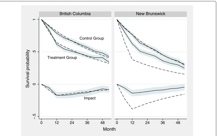
As a test of the importance of endogenous search intensity, we compare the Income Assis-tance survival probabilities, at six month intervals, for the control and program groups in the social experiment and in the model simulation graphically in Fig. 1 and with formal tests in Table 2. If search intensity were fixed, then the transition rate from IA to work should remain unchanged once the SSP is introduced in the partial equilibrium version of the model (i.e., holding the wage distribution, hours, job destruction and vacancies
Control Group
Treatment Group
Impact
−.5
0
.5
1
0 12 24 36 48 0 12 24 36 48
British Columbia New Brunswick
Survival probability
Month
Table 2Income assistance survival probabilities
British Columbia
Month Simulated Actual Simulated Actual
Control Control Program Program Simulated Actual
Group Group p-value Group Group p-value Impact Impact p-value
6 0.904 0.895 0.384 0.809 0.836 0.030 −0.095 −0.058 0.026 12 0.817 0.787 0.033 0.643 0.616 0.110 −0.175 −0.171 0.881 18 0.739 0.714 0.107 0.581 0.543 0.026 −0.158 −0.171 0.572 24 0.668 0.669 0.922 0.525 0.507 0.287 −0.143 −0.162 0.400 30 0.604 0.618 0.390 0.475 0.476 0.956 −0.129 −0.142 0.561
36 0.546 0.569 0.171 0.429 0.436 0.675 −0.117 −0.133 0.501 42 0.493 0.511 0.316 0.388 0.410 0.198 −0.105 −0.101 0.853 48 0.446 0.482 0.033 0.351 0.410 0.062 −0.095 −0.073 0.817 53 0.410 0.428 0.299 0.322 0.343 0.195 −0.088 −0.084 0.883
1–53 0.364 0.333
New Brunswick
Month Simulated Actual Simulated Actual
Control Control Program Program Simulated Actual
Group Group p-value Group Group p-value Impact Impact p-value
6 0.876 0.866 0.417 0.650 0.806 0.001 −0.226 −0.060 0.001
12 0.767 0.766 0.942 0.381 0.626 0.001 −0.386 −0.140 0.001 18 0.672 0.639 0.048 0.333 0.510 0.001 −0.338 −0.129 0.001 24 0.588 0.584 0.798 0.292 0.470 0.001 −0.296 −0.114 0.001 30 0.515 0.530 0.399 0.256 0.433 0.001 −0.260 −0.097 0.001 36 0.451 0.451 0.984 0.224 0.361 0.001 −0.227 −0.090 0.001
42 0.395 0.394 0.940 0.196 0.323 0.001 −0.199 −0.071 0.001 48 0.346 0.359 0.455 0.172 0.298 0.001 −0.174 −0.062 0.001 53 0.310 0.294 0.332 0.154 0.248 0.001 −0.156 −0.046 0.001
1–53 0.576 0.001
Note: p-values for single months are based on t-tests that the actual fraction still on IA minus the model prediction is equal to zero. For the all months test, we use a log-rank test that the actual (pooled) exits from IA are equal to the predicted (pooled) exits for the model and the data. The statistical tests treat the model predictions as constants
months after random assignment. For each month, we test the hypotheses that the model matches the experiment for the control group and for the program group, and the hypoth-esis that the simulated impact of the experiment matches the actual impact. The p-values for the joint hypothesis tests provide support for the model in this instance as the model is not significantly, or substantively, different from the experimental data at conventional significance levels.
As an additional test of how well the model predicts behavior, we reproduce a sec-ond experiment designed to estimate the delayed exit from Income Assistance that may result from the 12 month qualification period. The delayed-exit experiment was a sep-arate experiment conducted on a sample of 3,315 single parents in their first month of Income Assistance receipt in the metropolitan area of Vancouver, British Columbia. This sample was randomly assigned to program and control groups, where the program group was told that they would become eligible for the SSP program if they remained on Income Assistance for 12 months. The difference between the fraction remaining on Income Assistance in the program and control groups 12 months after random assignment is esti-mated by Ford et al. (2003) to be 3.9 percentage points with a standard error of 1.4. We conduct the same experiment in our model in partial equilibrium. The model predicts a delayed-exit effect of 4.3 percentage points in British Columbia, which is within one-third of one standard error of the effect estimated by Ford et al. (2003). The model is thus able to predict the magnitude of the experimental delayed-exit effect quite well. Comparing the model predictions with the experimental impacts, we can see that the model correctly predicts both the degree of delayed exit associated with the expectation of receiving the SSP benefit in the future (the entry effect) as well as the increased transition rate into employment that becoming eligible for the SSP program induces.
We come to a different conclusion upon examining the results for New Brunswick. As expected, the model provides a close fit to the control group. However, the simulated impact of the program on income assistance survival probabilities is significantly greater than that in the data. This is a substantial difference; the simulated impacts for months 12, 24, 36 and 48 are 2.76, 2.6, 2.52 and 2.8 times as large as the actual impacts. Our cur-rent parameterization of search intensity is not able to accurately predict the behavioral response to the introduction of the SSP in New Brunswick. We provide a more detailed explanation for this finding below.
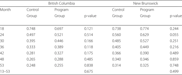
4.2 Job destruction
Table 3Employment survival probabilities, conditional on being employed in month 12 following random assignment
British Columbia New Brunswick
Month Control Program Control Program
Group Group p-value Group Group p-value
18 0.748 0.697 0.121 0.738 0.774 0.244
24 0.497 0.521 0.514 0.560 0.629 0.055
30 0.395 0.446 0.166 0.485 0.527 0.251
36 0.333 0.389 0.118 0.405 0.449 0.216
42 0.281 0.327 0.175 0.366 0.390 0.489
48 0.265 0.288 0.485 0.340 0.346 0.859
53 0.248 0.255 0.838 0.314 0.325 0.748
13–53 0.675 0.499
Note: p-values are for a t-test of equality of fraction still employed between the control and treatment group in the selected months. The test for months 13–53 is a log-rank test of equality of the survival functions, conditional on being employed in month 12
However, the data in Table 3 on both the program and control groups do not support the assumption of a constant job destruction rate. For both the program and control groups, the employment exit hazard rate is decreasing with the duration of employment in both provinces. There are several possible explanations behind this pattern. One possibility is that there is heterogeneity in job destruction rates across jobs; over time, the sample of remaining matches contains a disproportionate number of jobs with low destruction rates. Another possibility is that workers and firms learn about the true match value over time, so that low quality matches separate at a faster rate, as in Jovanovic (1979) and Jovanovic (1984).
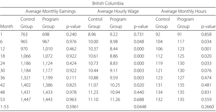
4.3 Earnings
One question of interest is whether earnings adjust in response to the introduction of an earnings supplement. In the partial equilibrium version of the model we consider, it is assumed earnings do not adjust to the policy change in the experiment because the number of individuals who receive the supplement is small. This assumption appears to be supported by the data, as there are no statistically significant differences between the (conditional on employment) earnings of the program and control groups in the exper-imental data in British Columbia and a significant difference only in month 6 for New Brunswick, as illustrated in Table 4.
Table 4Average earnings, wages and hours
British Columbia
Average Monthly Earnings Average Hourly Wage Average Monthly Hours
Control Program Control Program Control Program
Month Group Group p-value Group Group p-value Group Group p-value
1 763 698 0.240 8.96 9.22 0.731 92 91 0.858
6 965 967 0.976 10.00 8.98 0.048 104 117 0.034
12 970 1,010 0.462 10.37 8.44 0.000 106 123 0.001
18 1,066 1,072 0.922 10.61 8.86 0.000 112 125 0.020
24 1,186 1,124 0.424 10.73 8.83 0.000 119 130 0.033
30 1,184 1,177 0.922 10.44 9.11 0.003 121 130 0.076
36 1,321 1,199 0.111 10.88 9.59 0.003 123 127 0.474
42 1,402 1,386 0.825 11.07 10.25 0.020 131 135 0.481
48 1,431 1,433 0.978 11.23 10.94 0.440 134 135 0.831
53 1,447 1,443 0.963 11.10 11.26 0.688 132 135 0.559
1-53 0.5961 0.0448 0.2660
New Brunswick
Average Monthly Earnings Average Hourly Wage Average Monthly Hours
Control Program Control Program Control Program
Month Group Group p-value Group Group p-value Group Group p-value
1 547 491 0.240 5.98 6.07 0.770 94 87 0.171
6 613 732 0.002 6.40 6.33 0.799 100 116 0.001
12 726 759 0.476 6.50 6.29 0.374 111 121 0.027
18 775 798 0.553 6.80 6.19 0.008 113 129 0.000
24 797 845 0.281 7.10 6.47 0.012 113 128 0.000
30 839 862 0.617 6.99 6.62 0.094 117 128 0.017
36 839 853 0.749 7.13 6.72 0.067 113 126 0.002
42 902 929 0.526 7.13 6.95 0.381 123 131 0.063
48 932 971 0.346 7.31 7.23 0.680 125 134 0.021
53 923 990 0.134 7.45 7.60 0.492 122 130 0.061
1-53 0.1507 0.5801 0.0341
Note: p-values are for a t-test of equality of means between the control and treatment groups in the selected months. The joint test for months 1-53 is conducted by regressing the dependent variable on time and program status dummies. Observations with zero hours or wages are excluded
New Brunswick they work an extra 10 hours per month. By the time supplement pay-ments expire, there are no significant differences in wages or hours across the program and control groups. In addition, the joint tests suggest there are no significant differences in hours for British Columbia and wages in New Brunswick.36
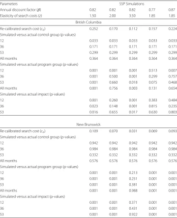
4.4 Sensitivity analysis
We next consider the sensitivity of our results to changes in the two parameters that are not calibrated to match data on the control group or Canadian labor force statistics:β andz. Both parameters were taken from the search literature, the former from a US study (Davidson and Woodbury, 1993) and the latter from estimates obtained using Danish data (Christensen et al., 2005). It is these two parameters that we therefore have the least confidence in. Table 5 presents evidence on the extent to which our results are sensitive to the choice of the discount factor (β) and the elasticity of search costs with respect to search effort (z). It is worth emphasizing that the search friction parametercais re-calibrated in the baseline model for each combination ofβandz. Lower values forβserve to reduce the incentives of individuals on unemployment and those on IA to search as the
Table 5Sensitivity to the choice ofβandz: IA survival probabilities
Parameters SSP Simulations
Annual discount factor (β) 0.82 0.82 0.82 0.77 0.87
Elasticity of search costs (z) 1.50 2.00 3.50 1.85 1.85
British Columbia
Re-calibrated search cost (ca) 0.252 0.170 0.112 0.157 0.224
Simulated versus actual control group (p-values)
12 0.033 0.033 0.033 0.033 0.033
36 0.171 0.171 0.171 0.171 0.171
53 0.299 0.299 0.299 0.299 0.299
All months 0.364 0.364 0.364 0.364 0.364
Simulated versus actual program group (p-values)
12 0.001 0.001 0.001 0.513 0.007
36 0.001 0.500 0.001 0.299 0.757
53 0.001 0.660 0.018 0.075 0.468
All months 0.001 0.756 0.003 0.131 0.654
Simulated versus actual impact (p-values)
12 0.001 0.260 0.001 0.383 0.484
36 0.023 0.148 0.001 0.815 0.235
53 0.016 0.655 0.017 0.630 0.803
New Brunswick
Re-calibrated search cost (ca) 0.109 0.070 0.031 0.069 0.093
Simulated versus actual control group (p-values)
12 0.942 0.942 0.942 0.942 0.942
36 0.984 0.984 0.984 0.984 0.984
53 0.332 0.332 0.332 0.332 0.332
All months 0.576 0.576 0.576 0.576 0.576
Simulated versus actual program group (p-values)
12 0.001 0.001 0.213 0.001 0.001
36 0.001 0.001 0.251 0.001 0.001
53 0.001 0.001 0.381 0.001 0.001
All months 0.001 0.001 0.988 0.001 0.001
Simulated versus actual impact (p-values)
12 0.001 0.001 0.371 0.001 0.001
36 0.001 0.001 0.431 0.001 0.001
53 0.001 0.001 0.922 0.001 0.001
value of employment falls. Lower values ofcaare then required to match the transitions into employment from Income Assistance. A similar argument holds forz. If search costs become more elastic (a higher value forz), then lower search costs are necessary to match the transitions into employment. The re-calibrated values forcaare presented in the top row of each panel in Table 5.
The remaining rows in Table 5 contain p-values for the following three hypothesis tests. First, we test whether the simulated survival rate for the control group in the model is equal to the survival rate for the control group in the data. Note that the p-values are the same for each parameterization. We recalibrate search costs whenβ andzchange to match the control group data and, as a result, can achieve the same fit in each case. Second, we conduct the same set of hypothesis tests for the program group. Finally, we test whether the simulated impact is equal to the experimental impact. Each test is conducted at 12, 36, and 53 months. We also test the hypothesis that the total number of exits up to month 53 is the same in the data and in the model.
In the case of British Columbia, the results indicate that the simulated control group does not match the experimental control group at the 12 month mark. Thus, the in-sample tests are able to rule out some aspects of all the parameterizations considered here. However, assessing whether the model fits the data based only on in-sample fit can be quite misleading. Two examples of this point are readily observed. First, in several cases the model fits the control group but cannot replicate the impact of the program. The set of results for the case wherez= 1.500 andβ= 0.820 for British Columbia is illustrative of this point. The model is able to match the control group at 36 and 53 months; how-ever, the model is not able to match the program group nor the experimental impacts in the data. In the absence of experimental data, we would be ignorant of the failure of the model to generate accurate predictions in this instance. This result highlights the fact that in-sample fit would not reject some parameterizations that our test would reject.
Second, in some cases, the simulated control group does not consistently match the data despite the fact that the model accurately predicts the impact of the SSP, as in the final column for British Columbia. It appears we are missing some features of the data that do not vary across the program and control groups and thus cancel out when computing the program impact. In this case, we may reject the model because of its inability to match the control group when in fact it is able to produce a good estimate of the program impact.
For New Brunswick, the sensitivity analysis indicates that the choice of a high elasticity of search costs with respect to effort provides a much better fit to the program group, with no change in fit to the control group. This result suggests that a combination of low search costs and a high value ofzis necessary to fit the data for New Brunswick. It is again clear that the experimental data provides us with useful information on the performance of the model under various parameterizations.
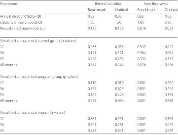
4.5 Using the extra variation introduced by the experiment
to use this additional variation in the calibration process. To this end, we conduct a grid search over zto determine what parameter values best fit the experimental impact in the data.37A comparison between the performance of our benchmark model and that of the ‘optimal’ calibration is presented in Table 6. For British Columbia, we find the ‘opti-mal’ parameter values are very close to the benchmark values and that we only make a small improvement in model fit by taking advantage of the experimental variation. In the case of New Brunswick, the optimal parameter values are quite different from the benchmark values. The results from the former province suggest that ignoring the exper-imental variation in the calibration process does not affect the predictive performance of the model; the results from the latter suggest the opposite. The fact that the conclusions across provinces are mixed, despite the fact that identical experiments were implemented in both provinces, is further evidence of the usefulness of our model test.
5 Conclusion
In this paper, we use social experiments as an innovative and rigorous test of a model’s ability to replicate observed behavior. In particular, we consider the ability of a standard search model, fit to an experimentalcontrol group, to match theprogram groupas a for-mal test of the model. Our results provide strong support for the model in this instance along some dimensions but not others. First, we use evidence on the impacts of the SSP on the IA-to-work transition rates during the 53 months following random assignment as a test of the specification for search intensity in the model. We find that the model pro-gram and control groups are not significantly, nor substantively, different from those in
Table 6Comparison of benchmark and optimal calibration: IA survival probabilities
Parameters British Columbia New Brunswick
Benchmark Optimal Benchmark Optimal
Annual discount factor (β) 0.82 0.82 0.82 0.82
Elasticity of search costs (z) 1.85 1.93 1.85 3.36
Re-calibrated search cost (ca) 0.185 0.176 0.079 0.033
Simulated versus actual control group (p-values)
12 0.033 0.033 0.942 0.942
36 0.171 0.171 0.984 0.984
53 0.298 0.298 0.332 0.332
All months 0.364 0.364 0.576 0.576
Simulated versus actual program group (p-values)
12 0.110 0.010 0.001 0.202
36 0.675 0.825 0.001 0.244
53 0.195 0.426 0.001 0.394
All months 0.333 0.994 0.001 0.998
Simulated versus actual impact (p-values)
12 0.881 0.551 0.001 0.359
36 0.501 0.261 0.001 0.424
53 0.883 0.841 0.001 0.929
the experimental data for British Columbia but are different for New Brunswick under our benchmark calibration. The model is also able to match the delayed-exit effects of a second randomized experiment that offered SSP to new Income Assistance recipients. Secondly, we find that the employment survival rates in the experimental data are consis-tent with an exogenous, but not a constant, job destruction rate. Our analysis also points to several extensions that may help in explaining other features of the data, including the joint determination of hours and wages.
It is important to emphasize two points. First, we could not draw this conclusion without the availability of experimental data. Our analysis highlights a second use of experimental data that has not been widely exploited in the literature. Second, the exper-imental data provide strong support for the search framework in this instance along certain dimensions, most notably the IA-to-work transition in British Columbia, the main margin over which the SSP is likely to influence behavior. Our model test indicates that the model captures the fundamental dynamics introduced by the SSP supplement. The data also support the use of the model in the case of New Brunswick, but under a much dif-ferent set of parameter values. Considering the widespread use of this model, the results provide support for the use of this framework to study policy changes that impact the labor market. It is very important, however, that future work considers the robustness of this result by exploiting other sources of variation.
It is also worth emphasizing that our model test involves a direct test of a partial equilibrium version of the model. The reason for this is simple: the social experiment is conducted on a small sample of individuals and therefore does not have spillover effects on the rest of the economy. As such, we do not have a direct test of the equilibrium implications of the potential policy change. That said, we take the fact that the partial equilibrium version of the model passes our more rigorous test as very convincing evi-dence in favor of using the model for British Columbia (but not for New Brunswick), as the model can replicate many of the outcomes produced by a social experiment with-out the use of the variation introduced by the social experiment. This finding increases our confidence in equilibrium policy evaluations and the evaluation of potential policies that can be conducted within the model but were not conducted within the experiment. In a companion paper (Lise et al. 2004) we use the model presented here to evaluate the potential spillover effects that may arise should the SSP be implemented as a policy on a wide scale for British Columbia. Lise et al. (2004) find that several important feedback effects, including displacement and changes in the equilibrium wage distribution, reverse the cost-benefit conclusions implied by the partial equilibrium experimental evaluation. Taken together, both papers illustrate that combining social experiments and models of the labor market and government assistance programs represents a powerful tool for policy evaluation.
Endnotes
1For example, see the evaluation of the Reemployment Bonus by Davidson and
DMP model. Others, such as Ljungqvist and Sargent (1998) and Alvarez and Veracierto (2000), have considered a variety of labor market policies using a modification of the McCall (1970) search framework. Hopenhayn and Rogerson (1993) consider policy evaluation in a calibrated equilibrium model using firm-level data.
2A very useful discussion of this and related issues can be found in Hansen and
Heckman (1996).
3See Kydland and Prescott (1996) for a detailed discussion.
4It is also possible to estimate a structural model on a subset of the data, for example a
subset of states, and use the remainder of the data to conduct a validation exercise. See Keane and Wolpin (2007).
5Crépon et al. (2013) provide experimental estimates of the equilibrium effects of
active labor market programs in France using a unique design that randomizes the fraction treated at the level of the labor market and individual treatment assignment within labor markets.
6The ability of the canonical DMP model to fit to the data has recently attracted much
attention. A large literature has now developed, starting from Shimer (2005) and summarized nicely in Mortensen and Nagypal (2007), on what model features are necessary for the DMP model to replicate aggregate fluctuations in productivity, unemployment and vacancies. The simplest version of the DMP model with Nash bargaining and homogeneous workers and firms does not produce much volatility in unemployment and vacancies in response to fluctuations in labor productivity. This can be overcome with, for example, alternative assumptions on wage determination (Hall 2005; Gertler and Trigari 2009) or worker and firm heterogeneity (Lise and Robin 2014). Recently Hornstein et al. (2011) illustrate quite clearly that without on-the-job search, this class of models produces very little in the way of wage dispersion.
7In parallel work, Todd and Wolpin (2006) use data from the experimental evaluation
of Mexico’s PROGRESA program to test a structural, dynamic model of fertility and child schooling using a similar approach. Bajari and Hortaçsu (2005) test a structural auction model using data from a laboratory experiment. Earlier work by Wise (1985) uses experimental data on housing subsidies to test a model of housing demand. More recently, Attanasio et al. (2012) use experimental data in the estimation of their
equilibrium model of PROGRESA, and Gautier et al. (2012) combine experimental data with data on non-participants from labor markets affected and not affected by the experiment to estimate the general equilibrium effects of a job search treatment using a differences-in-differences design.
8A large literature considers various aspects of the Self-Sufficiency Project, including
Bitler et al. (2008), Card and Hyslop (2005), Connolly and Gottschalk (2009), Ferrall (2012), Foley and Schwartz (2003), Kamionka and Lacroix (2008), Michalopoulos et al. (2005), Riddell and Riddell (2014), and Zabel et al. (2013). Similar, but less generous, income supplement programs have been studied in the United States; see Auspos et al. (2000) on the Minnesota Family Investment Program and Bos et al. (1999) on the Wisconsin New Hope program. Bloom and Michalopoulos (2001) provide an overview of the experimental literature and compare these programs to other approaches.
9We do not consider distributional effects of the policy change on earnings, as the
simple model is not well suited to doing so.
10Throughout this paper we use the term unemployed to mean collecting
unemployment benefits. In the model, all jobless individuals are actively seeking employment; they are distinguished by whether they are receiving unemployment benefits or Income Assistance benefits.
11The firm’s problem and the equilibrium conditions are outlined in detail in the
exceeds the value of being on IA or unemployed so that a match forms whenever a worker successfully contacts a firm.
12It is worth noting that we assume all Income Assistance recipients enter
employment with tenure zero. This assumption could be relaxed by assuming workers retain their experience when they enter Income Assistance and allowing experience to depreciate over time. One implication of this extension would be that the hazard of leaving IA would decline as the length of the IA spell increased. The drawback of this extension is that it involves a large increase in the size of the state space.
13Alternatively, we can consider the length of a period tending to zero and work in
continuous time, where there is zero probability of more than one application arriving simultaneously.
14Note that our matching function, as in Davidson and Woodbury (1993), exhibits
increasing rather than constant returns to scale. While this is a somewhat nonstandard assumption, it has no effect on our results since our tests are done in partial equilibrium. We could have equivalently assumed that the job contact probability is simply
proportional to search effort.
15In determining the marginal cost and benefit of search effortλis held constant under the assumption that each worker believes her impact is small relative to total labor supply.
16For comprehensive details on the Self-Sufficiency Project, see Michalopoulos et al.
(2002).
17In particular, individuals had to receive IA in the current month and in at least 11
out of 12 of the prior months to be included in the experiment.
18The selected areas were the lower mainland in British Columbia and the lower third
of New Brunswick.
19As noted in Lin et al. (1998), about 90 percent of the target population agreed to be
randomly assigned as part of the main (“recipient”) component of the SSP
demonstration that constitutes our primary focus in this paper. This leaves only modest scope for biases in the experimental impact estimates when interpreted as applying to the entire target population rather than just the study population of those who agree to random assignment. Kamionka and Lacroix (2008) consider the smaller “early entry” experiment, which we briefly consider in Section 4.1. It attracted only about 80 percent of its target population into random assignment. Their analysis suggests that this leads to a substantively meaningful understatement of the effects of the SSP treatment. Sianesi (2014) provides further useful discussion of these issues, an application to a more recent experiment, as well as pointers to the broader literature.
20No other sources of income affect the calculation of the earnings supplement.
21Out of the full sample of 6,208 individuals participating in the baseline interview,
2,849 individuals were assigned to the control group, 2,880 were assigned to the program group, and the remaining 299 were assigned to a third experimental group, the SSP Plus group. Thus, we are missing information on 464 respondents. A total of 40 respondents did not meet the criteria for inclusion in the experiment, and 3 control group members withdrew. An additional 398 individuals could not be contacted or refused to be interviewed. Lin, Robins, Card, Harknett, and Lui-Gurr (1998) consider the possible nonresponse biases that may arise and conclude the biases are likely to be small.
22The control group contains 815 recipients from New Brunswick and 856 from
British Columbia, while the program group consists of samples of 813 and 862 respondents from New Brunswick and British Columbia, respectively.
23“Without completed post-secondary education” refers to respondents reporting up
to some post-secondary education but no post-secondary certificate or higher. 24For example, the search intensity parameter (z) would only be identified off the
25Approximately 14 % of the control group in the Self-Sufficiency Project has at least
some post-secondary education: 11.3 % of the sample reports having some
post-secondary education and 2.2 % of the sample reports having a degree or certificate from a university.
26The standard full-time weekly hours in Canada is 37.5 hours.
27The Canadian Labour Force Survey is the analogue of the U.S. Current Population
Survey.
28All figures are reported in Canadian dollars, where $1Cdn was approximately equal
to $0.63US at the time of the experiment.
29This measure of job tenure does not take quits into account. As a result, we may
overestimate the job separation rate as individuals moving between jobs because of quits report holding jobs of shorter durations.
30See Lise et al. (2004) for further details.
31See Lin et al. (1998).
32The model changes required to introduce the SSP are minor. Full details on the
augmented model are presented in the Appendix.
33For example, this means thatλdoes not change when we introduce the program in partial equilibrium. We also assume that the introduction of the SSP is not anticipated by individuals in the simulated program group.
34See Mortensen and Pissarides (1994) for a model with endogenous job destruction.
35See the notes at the bottom of Table 3 for full details.
36As noted by Card and Hyslop (2005) and Zabel et al. (2013), the fact that wages can
only be compared for those members of the program and control groups that work may be problematic. In the spirit of most relatively simple search and matching models in the DMP tradition, we ignore issues surrounding unobserved heterogeneity in this paper.
37The grid is overz∈ {1.50, 3.50}with an interval size of 0.005. We do not search over
bothβandz, as the discount factor is not separately identified from search costs. For each value ofzwe consider, the search costs parametercais recalibrated to match the IA survival function for the control group. Our measure of best fit is the maximum p-value for the joint test (all months) of simulated versus actual impacts for IA survival
probabilities.
38We assume for simplicity that individuals entering employment from unemployment
with remaining benefit months available start accumulating benefit months immediately. 39If the individual’s earnings are above the ceiling, they do not receive a supplement.
For simplicity, we abstract from this case within the model as few individuals had earnings above the supplement ceiling in the data. In the model no individuals have earnings above the supplement ceiling.
40In the actual SSP experiment, once individuals qualified for the earnings supplement
they could transit between employment and IA and collect the supplement payments in any month they were employed full-time during the 36 months after qualifying. We abstract from this in the model as it would add an unmanageable number of states. Instead, we allow those who lose their job prior to qualifying for unemployment benefits to transit back to the first period of SSP eligibility.
41It is assumed thatI<T
end, which is consistent with the actual EI and IA programs. 42Production takes place when there is a match between one firm and one worker; the
number of firms can alternatively be interpreted as the number of jobs in the economy. 43Alternatively, we can consider the length of a period tending to zero and work in
continuous time, where there is zero probability of more than one application arriving simultaneously.
44In determining the marginal cost and benefit of search effortλis held constant under the assumption that each worker believes her impact is small relative to total labor supply.
Appendix A: The basic model
A.1 Firms
Production takes place when there is a match between one firm and one worker; the number of firms can alternatively be interpreted as the number of jobs in the economy. There is free entry in the economy. In every period, each firm has the option of filling a vacancy, if one exists, by hiring a worker or keeping the vacancy open. If matched with a worker, firms earn profits that depend on the surplus generated by the match and pay wages, determined in equilibrium, that depend on the worker’s outside options and the minimum wage. Profits depend on the worker’s tenure to allow match-specific capital to increase the productivity of the match over time. Denote the surplus generated by a worker-firm pair of tenuretbyS(t). With probabilityδthe match separates and the firm is left with a vacancy in the following month. Denote the profits of a firm matched with a worker with outside optioni,i∈ {0, 1,. . .,u,. . .,u¯}and match tenuretas(t,i).
The expected discounted present value of profits for matches of job tenure t and workers with outside optioniare
E(t,i)=S(t)−w(t,i)+ ⎧ ⎪ ⎪ ⎪ ⎪ ⎪ ⎪ ⎪ ⎪ ⎨ ⎪ ⎪ ⎪ ⎪ ⎪ ⎪ ⎪ ⎪ ⎩
β[δV +(1−δ)E(t+1, 0)] ifi=0 andt<I, β[δV +(1−δ)E(t+1,u)] ifi=0 andt=I, β[δV +(1−δ)E(t+1,i+1)] if 0<i<u¯andt<T, β[δV +(1−δ)E(t+1,u¯)] ifi= ¯uandt<T, β[δV +(1−δ)E(T,u¯)] ift≥T,
where match tenure beyondTno longer increases profits.
If a firm has a vacancy, the value of the vacancy is determined by the probability of meeting an unmatched worker, by the profits the firm expects to make from the match, and by the costs of posting a vacancy (ξ)
V = −ξ+β u¯
i=0
q(i)E(1,i)+
1−
¯
u
i=0 q(i)
V
,
whereq(i)is the probability a firm matches with a worker with outside optioni.
A.1.1 Matching probabilities
From the firm’s perspective, the probabilities of meeting potential workers from unem-ployment and IA equal the fraction of workers from unemunem-ployment and IA who transit to employment, divided by the total number of vacancies
q(i)= m(i)U(i)
V and q(0)=
m(0)A V , respectively.
A.2 Equilibrium wage determination
outside option, which depends on their current labor market state and program eligibil-ity. The surplus from the perspective of the firm is the difference between the profits the firm receives at the equilibrium wage and the value of leaving the vacancy open. It is fur-ther assumed that the bargaining process is constrained such that the wage can not fall below the minimum wagew. The equilibrium wage is max{w(t,i),w}, wherew(t,i)solves
VE(t,i)−Vi=E(t,i)−V,
whereVi ∈ {VA,VU(i)}is the value of the outside optioni. In the following section, we define the steady state conditions for employment, unemployment, and IA.
A.3 Steady state conditions
LetEdenote the steady state number of jobs occupied by workers andV the number of vacancies. By definition, the total number of jobs in the labor market is equal to the total number of occupied jobs and the total number of vacancies
F=E+V.
Denote the total number of individuals in the labor market byL. The total number of indi-viduals can be decomposed into three groups. First the employed, who are distinguished both by their current job tenure and their current outside option
E= T
t=1
¯
u
i=0
E(t,i)+ ¯E,
whereE¯ is the group of workers no longer experiencing on-the-job wage growth. The second group, denotedA, consists of individuals on Income Assistance. The final group are unemployed individuals (U)
U=
¯
u
i=1 U(i),
where U(i) indicates the number of unemployed persons with i periods of benefits remaining.
The total number of individuals in the labor market can therefore be expressed as the sum of the above components
L=E+A+U.
Using the above definitions, we can describe the conditions governing the steady state, where the flows in and out of every employment state must be equal over time. The steady state conditions for each state and eligibility combination are discussed in turn below.
A.3.1 Employment