DOI 10.1007/s13174-012-0073-z O R I G I NA L PA P E R
Computing multicast trees in dynamic networks
and the complexity of connected components in evolving
graphs
Sandeep Bhadra · Afonso Ferreira
Received: 30 August 2011 / Accepted: 8 October 2012 / Published online: 6 November 2012 © The Brazilian Computer Society 2012
Abstract Future Internet technologies and the deployment of mobile and nomadic services enable complex commu-nications networks, that have a highly dynamic behavior. This naturally engenders route-discovery problems under changing conditions over these networks, but the tempo-ral variations in the topology of dynamic networks are not effectively captured in a classical graph model. In this paper, we use evolving graphs, which help capture the dynamic characteristics of such networks, in order to compute mul-ticast trees with minimum overall transmission time for a class of wireless mobile dynamic networks. We first show that computing different types of strongly connected com-ponents in evolving digraphs is NP-Hard, and then propose a polynomial-time algorithm to build all rooted directed Minimum Spanning Trees in strongly connected dynamic networks. These results open new avenues for the implemen-tation of Internet spanning-tree based protocols over highly dynamic network infrastructures.
Keywords Future internet· Graph theoretic models· Dynamic networks·Wireless networks·Routing·Evolving graphs·Minimum spanning trees
Sandeep Bhadra
Department of Electrical Engineering, Indian Institute of Technology, Madras, Chennai, India
e-mail: [email protected] Afonso Ferreira (
B
)CNRS, I3S, INRIA-Sophia Antipolis, Projet MASCOTTE, BP93, 2004 Rt. des Lucioles, 06902 Sophia Antipolis, France
e-mail: [email protected]
1 Introduction
With the advent of the Internet of Things, it is clear that a glob-ally mobile Internet induces key new challenges related to existing communication and routing solutions [2]. As stated in [15], a major challenge for the Future Internet, where most connected entities will be mobile, is the explicit design of protocols for a mobile wireless world.
Indeed, infrastructure-less mobile communication envi-ronments, such as mobile ad hoc networks (MANETs), present a paradigm shift from back-boned networks in that data are transferred from node to node via peer-to-peer inter-actions and not over an underlying backbone of routers. Naturally, this engenders new problems regarding optimal routing of data under various conditions over these dynamic networks [18].
In this setting, the generalized case of mobile network routing using shortest paths or least cost methods are com-plicated by the arbitrary movement of the mobile agents thereby leading to random variations in link costs and con-nectivity [18]. This variable nature of the topology can be apprehended only by network updates of the link state between moving nodes, thus creating substantial commu-nication overhead along the link. This naturally motivates studying the modeling of such dynamics, and designing algo-rithms that take it into account [19].
Literature related to route discovery issues in dynamic networks started more than four decades ago, with papers dealing with operations of transport networks (e.g., [7,11– 13]). Work on time-dependent networks deals with flow algo-rithms in static networks, with edge traversal times that may depend on the number of flow units traversing it at a given moment. If traversal times are discrete, then the approach pro-posed in [11], namely of expanding the original graph into
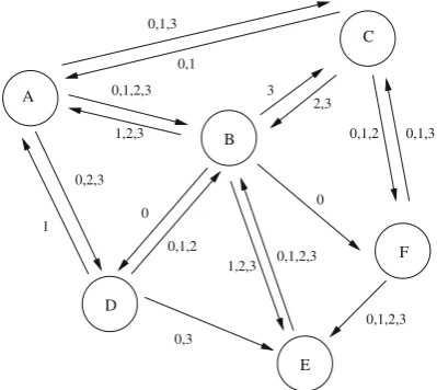
Fig. 1 An FSDN represented as an indexed set of networks.The indices correspond to successive time-steps comp00comp01comp02 comp03
approach), may work for computing several path-related problems (see [16,17] and references therein). Unfortunately, this approach leads to non-tractable algorithms, sinceT may be of exponential size.
1.1 Predictable dynamics
Note, however, that for the case of low earth orbiting (LEO) satellite systems, unmanned aerial vehicles (UAV), and other mobile networks with predestined trajectories of the mobile agents, the network dynamics are somewhat deterministic. Therefore, since the trajectories of the network agents are known in advance, it is possible to exploit this determinism in optimizing routing strategies [8,10,20].
Another setting where the evolution of the network is known was studied in [9]. The authors used the notion of com-petitive analysis [3] on a dynamic setting in order to analyze the quality of a protocol and its online choices made, forced by the evolution of the network. At the end of the process, the
historyof the network is formalized as a sequence of graph topologies on which the application can be solved off-line. Themeritof the protocol is then the ratio of the solution cost found online over the optimal off-line cost.
Such networks, where the topology dynamics is known or can be predicted beforehand, are henceforth referred to as
fixed schedule dynamic networks(FSDNs) (see Fig.1).
1.2 Evolving graphs
Evolving graphs are a formal abstraction for dynamic net-works, and can be suited easily to the case of FSDNs [4]. Concisely, an evolving graph is an indexed sequence ofT subgraphs of a given graph, where the subgraph at a given index point corresponds to the network connectivity at the time interval indicated by the index number. The time domain
0,1,2,3 3
0,1,2,3
1,2,3
1 0,2,3
0,3 0
1,2,3 0,1,2
0,1,3 0,1,2 0,1,3
0,1
0,1,2,3 A
B
C
D
E
F 0
2,3
Fig. 2 Evolving digraph corresponding to the FSDN in Fig.1. Edges are labeled with corresponding time-steps. Observe thatC B Fis not a valid journey sinceB Fexists only in the past with respect toC B
is further incorporated into the model by restrictingjourneys
(i.e., the equivalent of paths in usual graphs) tonevermove into edges which existed only in past subgraphs (cf. Fig.2 below, and Sect.2). We refer to evolving digraphs to indi-cate the fact that the edges are directed, implying the same distinction that exists between graphs and digraphs.
Notice that this model allows for arbitrary changes between two consecutive time steps, with the possible cre-ation and/or deletion of any number of vertices and edges. Evolving graph edges can also be associated with traversal times. In [4], algorithms were proposed for findingforemost, shortest, andfastestjourneys in dynamic mobile networks modeled by evolving graphs. Other path problems in evolv-ing graphs can be found under themeritapproach [9]. Results proven include finding a sequence of paths that connect a given pair of nodes throughout the system, such that the global routing plus re-routing costs are minimized.
1.3 Our work
our approach differs from these, in that our algorithm builds DMSTs over dynamic mobile networks modeled by evolv-ing digraphs, which can be seen as dynamically changevolv-ing digraphs.
In this paper, we start by providing, in the next section, basic definitions for various common graph theory terms in the context of evolving digraphs. Following Humblet [14], we define rooted DMSTs over strongly connected evolv-ing digraphs. This naturally leads to the question of how to determine if an evolving digraph is strongly connected. In Sect.3, we define strongly connected components (SCCs) in evolving digraphs and discover that the unique properties of evolving digraphs yield two types of strongly connected components: standard SCCs and the more loosely defined open strongly connected components (o-SCCs), as it will become clear later. One of our results is that unlike in stan-dard digraphs, finding the strongly connected components in evolving digraphs is not possible in deterministic polynomial time, unless P=NP. In case the evolving digraph is already identified as a strongly connected component, we give in Sect. 4 a polynomial-time algorithm to compute DMST, which uses a variation of Prim’s algorithm [6] for computing minimum spanning trees. For an evolving digraph with N
nodes and maximum outdegreeD, our algorithm builds the rooted DMST over a strongly connected component in an evolving digraph inO(NDlogT)time. Section5contains concluding remarks and scope for further research.
2 Graph theoretic model
Since we use evolving digraphs as a model for FSDNs throughout this paper, we start with a revision of the basic definitions of terms in the theory of evolving digraphs.
2.1 Evolving digraphs
Evolving digraphs are defined as follows.
Definition 1 (Evolving Digraphs) Let a digraph G(V,E)
be given, along with an ordered sequence of its subdigraphs, SG = G0,G1, . . . ,GT,T ∈ IN. Then, the system G =
(G,SG)is called an evolving digraph.
We now define some of the main parameters of an evolving digraph. Let EG = Ei, andVG =
Vi. It is clear that
M= |EG| ≤ |E| = M and thatN = |VG| ≤ |V| = N.
The central notion in evolving graph theory is the restriction imposed upon paths to traverse arcs strictly in non-decreasing order of arc schedule times, implying that there are no paths inGgoing to the “past”.
Definition 2 (Journeys) Let P be a path inGi, under the usual definition. Let F(P)be its first vertex, L(P)be its
last vertex, and|P|be its length. We define ajourney inG
between two verticesuandvofVGas a sequenceJ(u, v)= Pt1,Pt2, . . . ,Ptk, witht1<t2<· · ·<tk, such that Pti is a
(usually defined) path inGti withF(Pt1)=u,L(Ptk)=v,
and for alli <kit holds thatL(Pti)=F(Pti+1).
Corresponding to each arc in EG we may define anarc scheduleas a set of indices indicating the presence of the arc in the respective subdigraphs inSG. Thus, we may alternately define an evolving digraph as a tupleG=(VG,EG), where each arc inEGhas an arc schedule defined for it.
Two vertices are said to beadjacent inG if and only if they are adjacent in someGi. The degree of a vertex inGis defined as its degree inEG.
As usual, a tree in G could be defined as a connected induced subdigraph ofVGwith no circuits inG(V,E). How-ever, such a tree would not be very helpful when studying connectivity issues, since it does not take into account the total order of the subdigraphs in G, and the restrictions it imposes on journeys inG. Therefore, we define avalid rooted tree inGas a rooted directed tree inG, where all paths from the root to the leaves are journeys inG.
2.2 Strongly connected components and arborescences
We define an evolving digraphGto be astrongly connected
digraph if there exists a journey J inG between any two vertices inVG.
Definition 3 (Strongly Connected Component) Analogous to standard digraphs [6], we define astrongly connected
com-ponent(SCC) in an evolving digraph as a maximal set of
verticesUG ⊆ VG such that for any pairu, v ∈ UG, there exists a journey fromutovand fromvtouusing only arcs in the Cartesian productUG⊗UG.
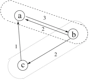
Thus, the subdigraphGinduced by considering vertices in the SCCUGis a strongly connected digraph. For example, in Fig.3,{b,a}forms a SCC since there are journeys fromato
a
b
c
12 3 2
Fig. 3 Open strongly connected components. Arcs are labeled with their respective arc schedule times
A journey between two nodesu, v ∈UG, might need to use nodeshi ∈VG,hi ∈/UGto maintain strong connectivity. The set of such nodes{hi} =H(u, v)are the helping nodes (h-nodes) for the verticesu, v.
Consequently, an SCCUGis an o-SCC with the additional requirement that H(u, v) = ∅ ∀u, v ∈ UG. Hence, the set
{b,c}in Fig.3forms a o-SCC withH(b,c)= {a}since ver-texais required to form the only journey frombtoc, thereby maintaining strong connectivity. Also, since H(b,c) = ∅,
{b,c}is not an SCC.
For the case of static networks, Humblet [14] defines the concept of rooted spanning trees over strongly connected directed networks. We extend this definition to the case of evolving digraphs as follows. We define arooted directed spanning treeor anarborescenceover a o-SCCUG ∈Gas a valid rooted directed tree inGrooted atr which spans all the vertices inUG; thus, all the nodes except the root has one and only one incoming arc. Note that the arborescence might need to includeh-nodes to reach some vertices in the o-SCC.
3 Complexity of strongly connected components
In this section we will first use the foremost journey algo-rithm to verify strong connectivity for an FSDN. Then we will prove that the decomposition of a FSDN into (o-) SCC components is NP-Hard.
3.1 The network model
A FSDN can be seen as a series of networks R =
. . . ,Rt−1,Rt,Rt+1, . . .over time. We model a FSDN as a
dynamic network which has apresencematrixPE[(u, v),i], indicating whether(u, v)is present at time stepti, for each link(u, v)ofR, and anotherpresencematrixPV[u,i], indi-cating whether u is present at time step ti, for each node
u of R. The network at timeti is then represented by the subnetworkRt ofR, which is obtained by taking the nodes
and links ofRfor which their corresponding P[i]s indicate they are to be present.
In order to model a fixed-schedule dynamic network by an evolving digraph, it suffices to be given a time windowW of sizeT, and to work withG=(Ri|i ∈W,FSDN|W). Throughout this text, we assume packet-based networks—so transmitting one piece of data equals transmitting one packet over an arc. Link transmission time between nodes in the net-work may allow for the transmission of a packet over several links before a change in the network topology. Correspond-ingly in the model, considering time between two succes-sive subdigraphs in an evolving digraph as unity, the time taken to cross an arc(u, v)is expressed as a positive delay
w(u, v) ≤ 1. The case where the traversal time is larger than the frequency of topology change would then yield a delayw(u, v) >1. We also implicitly assume conservation of information, i.e., in case a node in the network disappears for any reason, then upon rejoining the network, it will still have all the information that it had received before its disap-pearance.
3.2 Verification of strong connectivity in FSDNs
Given an FSDN network, we must determine if it is strongly connected. It is equivalent to the following proposition over the corresponding evolving digraph.
Proposition 1 Given an evolving digraphGwithN nodes
and M links over a sequence of length T, it is
pos-sible to determine if it is strongly connected or not in O(N M(logT +logN))time steps.
Proof Thetransitive closureofGis defined as the digraph
RG=(V,ER),whereER={(vi, vj): ∃a journeyJ(vi, vj)}. Hence,G is strongly connected if the underlying graph of
RGis a complete graph1. The verification is executed simply and efficiently by forming the foremost journeys tree for each node in the network using the algorithm for a single node pro-posed in [4], whose complexity isO(M(logT+logN)). For N nodes, the algorithm is repeatedN times, for an overall time ofO(N M(logT +logN)).
3.3 Decomposition into SCCs
Tarjan’s algorithm [6], based on the concept offorefathersin a depth-first search tree over a digraph, is used to decompose standard digraphs into SCCs. However, SCCs in evolving digraphs have the following unique properties, which pre-clude the use of Tarjan’s algorithm.
1 The underlying graph ofR
Grefers to the undirected graph that has an edge betweenviandvjif and only ifERhas both arcs(vi, vj)and
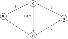
a
b c
d
1
2 3
4
5 6
7 , ,
Fig. 4 Overlapping SCCs. Arcs are labeled with their respective arc schedule times
Property 1 Two different SCCs can have common vertices.
For example, consider the digraph given in Fig.4. From the definition of SCCs we see that there are two SCCsa,c,d
andb,c,d which have the verticesc,din common. Property 2 For any two vertices in an SCC (respectively, o-SCC), there may be journeys connecting them which use vertices outside the SCC (respectively, o-SCC).
This stands directly from Property 1. As an example, con-sider in Fig.4the journey fromd toc, which uses vertexa
that lies outside the SCC{b,c,d}.
The main problem calls for decomposing the evolving digraph into all possible SCCs. Consider a subproblem
COM-PONENTdefined as follows.
COMPONENT: Given an evolving digraphG=(VG,EG)
and an integerk, is there a SCC of sizek?
We shall subsequently demonstrate thatCOMPONENTis NP-Complete, thereby precluding a polynomial time algo-rithm for the decomposition problem, unless P=NP.
Theorem 1 COMPONENT is in NP.
Proof Given a subsetVG ofVGand an integerk, we must verify in polynomial time ifVG is indeed a SCC of sizek. First, verifying that|VG| = kis easy. Then, verifying that the subdigraphGinduced byVGonGis strongly connected is possible in polynomial time from Proposition1.
We now define astrong reachability digraphfor an evolv-ing digraphGas an undirected graphSG=(VG,ES), where
ES = {(vi, vj)}if and only if(vi, vj)∪(vj, vi)⊆RG, the transitive closure digraph ofG.
To prove the NP-Completeness of COMPONENT we reduce the CLIQUEproblem to COMPONENT. CLIQUE
is formally defined as follows: Given a digraphG=(V,E), and an integerk, is there a clique of sizekinG?
Lemma 1 Finding an SCC inG is equivalent to finding a maximal clique in SG, the strong connectivity graph ofG. Proof Directly from the definitions of strong reachability, SCC and maximal clique, we see that the SCC inGis equiv-alent to finding the maximal clique inSG. Theorem 2 CLIQUE can be reduced to COMPONENT in polynomial time.
Proof Given an undirected graphG=(V,E)and the integer
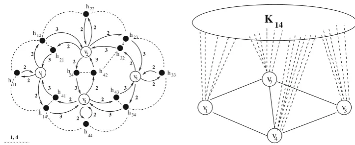
k, we construct an evolving digraphG=(VG,EG)as follows (cf. Fig.5):
1. For each nodeui ∈ V create a nodevi ∈ VG, a node
hii ∈ VG, and arcs(vi,hii), (hii, vi)with arc schedule time 2;
2. For each edge{ui,uj} ∈ E, do
(a) create nodeshi j,hj i ∈VG,
(b) create arcs(vi,hi j)and arcs(vj,hj i), with arc sched-ule time 2,
(c) create arcs(hi j, vj)and arcs(hj i, vi), with arc sched-ule time 3.
3. Create an SCC connecting allh-nodes. Label these arcs with schedule times 1 and 4.
By construction ofG, its corresponding strong reachability digraph SG contains a clique of size formed by all the
h-nodes. Letndenote its size. We can then prove that find-ing an SCC inGis the same as finding a clique inG, since a clique of sizekinGwill correspond to a clique of sizen+k
inSG, corresponding, in turn, to an SCC of sizen+kinG
(via Lemma 1).
Theorem 3 COMPONENT is NP-complete.
Proof We know that CLIQUE is NP-Complete. So from
Theorems 1and2,COMPONENTis NP-Complete.
3.4 Decomposition into o-SCCs
Here, we address the more general result for the case of o-SCC which has a less strict definition than SCC. We define the decision problem as follows.
o-COMPONENT: Given an evolving digraph G and an
integerk, is there a o-SCC of sizek?
Although SCCs are a special case of o-SCCs, the NP-Completeness ofCOMPONENTdoes not directly imply that
o-COMPONENTis NP-Complete as well. This is because
a possible polynomial time algorithm foro-COMPONENT
need only answer the above decision problem and not iden-tify the o-SCCs of sizek, thus making it difficult to verify if at least one o-SCC of sizekis an SCC as well (in other words if the set of h-nodes is empty or not for a particu-lar o-SCC of sizek). Also, the same digraphGmay contain both an SCC (of indeterminate size) and an o-SCC of sizek,
so o-COMPONENT would always return “yes”, ignoring
the presence or absence of a SCC of sizek, thereby
leav-ing COMPONENT unsolved. Conversely, since SCCs are
a special case of o-SCCs, proving o-COMPONENT to be NP-Complete does not directly imply thatCOMPONENTis NP-Complete as well.
how-Fig. 5 Construction for Theorem2. Arcs are labeled with their respective arc schedule times.
v
v
v
v
h12
h
h
h
h
h h h
22
33 21
34 43
23
32
h
h 11
14 41 h 1
h
h h
3
4
44 2
24 42
2 2
2 2
2 2
2 2 2
2
2
2 2 2
2 2 3
3
3
3 3
3 3
3
1, 4
2
3 2
3
K
14v
v
v v
1
2
4
3
ever, the same widget utilized for the previous reduction can be applied in the current case, yielding the following results.
Theorem 4 o-COMPONENT is in NP.
Proof The proof of this result is analogous to the one of Theorem 1. It can be derived step by step from the pre-vious proof, but showing it here would be quite fastidious and would not add new insights to this paper. Consequently, we leave the full development of this proof to the interested
reader.
Theorem 5 CLIQUE can be reduced to o-COMPONENT in polynomial time.
Proof Given an undirected graphG=(V,E)and the integer
k>3, the same arguments used in the proof of Theorem2 apply here. Indeed, the same widget can be used to reduce
CLIQUEto o-SCC, since a SCC is a o-SCC where H = ∅,
and in that widget, a max o-SCC is a max SCC, which by Theorem2implies the reduction fromCLIQUE.
Theorem 6 o-COMPONENT is NP-complete.
Proof We know that CLIQUE is NP-Complete. So from
Theorem 4 and Theorem 5, o-COMPONENT is
NP-Complete.
4 Computing directed Minimum Spanning Trees
Considering a strongly connected evolving digraphG, the object is to findN = |VG|rooted directed Minimum Span-ning Trees rooted at each of the nodesr∈VG. Our algorithm is a modification of the Prim–Dijkstra algorithm [6] for find-ing MSTs in undirected graphs. The algorithm proceeds by building a fragment which is a subset of the DMST starting from the rootr. The property of the fragment f(r)is that it consists of those edges by which information transmitted at the beginning of the time interval from the rootrwill travel in the shortest time to the vertices already included in the frag-ment. Having defined a fragment as such, it is easy to see how the algorithm for the DMST proceeds. In the following algo-rithm we choose from among the set of arcs outgoing from
the fragment f(r), the arc with the smallest arc schedule time such that it can form a valid journey starting from the root. A numbertv is associated with each vertexv ∈ VG denot-ing the minimum time required for that vertex to receive the information given that the rootroriginates the information. Since each node can transmit information only after it has received it, the information cannot pass simultaneously through two edges. Recall that the time required for trans-mission over one arc is denoted as an arbitrary weight,
w(u, v) <1.
In Algorithm 1, an arc schedule timeiindicates the pres-ence of the link from timei−1 toi.
Note that two cases might arise depending on whether
fa(uj, vj) = tuj + w(uj, vj) or fa(uj, vj) > tuj +
w(uj, vj). For the first case, the information reaches the node exactly at the time fa(uj, vj). For the other case, if the arc is present both at times fa(uj, vj)−1 and fa(uj, vj), since
w(uj, vj) <1, the packet will reachvj intuj +w(uj, vj).
If, however, the arc is not present at time fa(uj, vj)−1, then the transmission process itself starts at the fa(uj, vj)t h step (i.e., from time fa(uj, vj)−1 to time fa(uj, vj)), thus reachingvjby time fa(uj, vj)−1+w(uj, vj).
VGmust be replaced byVG and correspondingly, Step 3 of Algorithm 1 should be modified toVG ⊂Vf since the frag-ment can also contain the h-nodes for the vertices inVGand the loop can stop once all the vertices are covered.
Algorithm 1 is a greedy algorithm that always chooses the arc that transmits in minimum time. The proof of its cor-rectness is the same as the proof of the Prim–Dijkstra algo-rithm [6]. If the maximum outdegree of each vertex isD, then each step of increasing the fragment will takeO(N DlogT) time and the fragment will increaseN times adding up to a total execution time ofO(N2DlogT)steps.
5 Conclusion
The two important results in this paper are the intractability of the decomposition into (open) strongly connected com-ponents in FSDNs and the construction of DMSTs over an already existing strongly connected components. Note also that the very concept of Open Connected Components is completely new, and somewhat surprising, arising because of the dynamics of the networks, and may find important applications.
The former result implies that it is possible to lead a non-strongly connected network towards strong connectedness by adding intermediary agents to serve as hops between two nodes that are out of range from each other. An interest-ing problem would be to find a way to add such links so as to minimize the number of intermediary (helping) nodes. Another way for further research is to design approxima-tion algorithms for (open) strongly connected components in evolving digraphs.
Finally, the construction of minimum spanning trees in networks is part of the solution of many networking prob-lems, like that of finding a low-cost sub-network connecting a set of nodes. We are confident that the foundations laid by this paper will help understand the impact of mobility in networks of the future. The algorithms shown in this paper provide an efficient basis for the deployment of the Future Internet on highly dynamic network environments.
As possible avenues for future work, we know that in order to be more representative of reality, restrictions on network topology changes between consecutive time-slots may be introduced. In the case of mobility, such restrictions could be of geometric nature, e.g., dependent on expected speed and location of nodes. Such modeling of network dynamics could lead to the development of further algorithms, in addi-tion to the general-case and centralized algorithm presented in this paper. Distributed algorithms for this problem also need to be designed.
Acknowledgments The authors are grateful to Aubin Jarry and Stephane Perennes for very fruitful discussions. The authors would also like to thank the reviewers, in particular Reviewers 2 and 3, for the very
careful reading of the document. Their comments helped to increase the quality of this paper.
References
1. Ambuehl C (2005) An optimal bound for the MST algorithm to compute energy efficient broadcast trees in wireless networks. In: Proceedings of 32th ICALP, pp 1139–1150
2. Andersen FU, Berndt H, Abramowicz H, Tafazolli R (2007) Future internet from mobile and wireless requirements perspective.http:// www.emobility.eu.org/
3. Borodin A, El-Yaniv R (1998) Online computation and competitive analysis. Cambridge University Press
4. Bui-Xuan B, Ferreira A, Jarry A (April 2003) Computing shortest, fastest, and foremost journeys in dynamic networks. Int J Found Comput Sci 14(2):267–285
5. Chu YJ, Liu TH (1965) On the shortest arborescence of a directed graph. Sci Sin 14:1396–1400
6. Cormen T, Leiserson C, Rivest R (1990) Introduction to algorithms. The MIT Press, Boston
7. Dreyfus SE (1969) An appraisal of Some Shortest-Path Algorithms. Oper Res 17:269–271
8. Ekici E, Akyildiz IF, Bender MD (2000) Datagram routing algo-rithm for LEO satellite networks. In: IEEE Infocom, pp 500–508 9. Faragó A, Syrotiuk VR (2001) MERIT: a unified framework for
routing protocol assessment in mobile ad hoc networks. In: Pro-ceedings of ACM Mobicom 01, pp 53–60, ACM
10. Ferreira A, Galtier J, Penna P (2002) Topological design, routing and handover in satellite networks. In: Stojmenovic I (ed) Hand-book of wireless networks and mobile computing, pp 473–493. Wiley, New York
11. Ford LR, Fulkerson DR (1958) Constructing maximal dynamic flows from static flows. Oper Res 6:419–433
12. Halpern J (1977) Shortest route with time dependent length of edges and limited delay possibilities in nodes. Zeitschrift für Oper Res 21:117–124
13. Halpern J, Priess I (1974) Shortest path with time constraints on movement and parking. Networks 4:241–253
14. Humblet PA (1983) A distributed algorithm for minimum weight directed spanning trees. IEEE Trans Commun COM-31(6):756– 762
15. Issarny V, Georgantas N, Hachem S, Zarras A, Vassiliadis P, Autili M, Gerosa MA, Ben Hamida A (2011) Service-oriented middle-ware for the future Internet: state of the art and research directions. J Internet Serv Appl 2(1):23–45
16. Köhler E, Langkau K, Skutella M (2002) Time-expanded graphs for flow-dependent transit times. In: Proceedings of ESA’02 17. Köhler E, Skutella M (2002) Flows over time with load-dependent
transit times. In: Proceedings of the 13th annual ACM-SIAM sym-posium on discrete algorithms, pp 174–183
18. Scheideler C (2002) Models and techniques for communication in dynamic networks. In: Alt H, Ferreira A (eds) Proceedings of the 19th international symposium on theoretical aspects of computer science, vol 2285. Springer, pp 27–49, March 2002
19. Stojmenovic I (ed) (2002) Handbook of wireless networks and mobile computing. Wiley, New York
20. Syrotiuk V, Colbourn CJ (2003) Routing in mobile aerial net-works. In: Proceedings of WiOpt’03—modeling and optimization in mobile, ad-hoc and wireless networks, pp 293–302, INRIA, Sophia Antipolis, March 2003