Impact Of Innovative Environment On
Economic Growth: An Examination Of
State Per Capita GDP And Personal Income
Oi Lin Cheung, Indiana University East, USA
ABSTRACT
This study investigates how the overall innovative environment will affect the economic growth of a place, in particular, a state. Using the Innovation Index and its component indexes as a measure of the innovative environment prevailing in the states, it is found that the more innovative a state is, the higher its per capita real GDP and per capita personal income are. These relations are statistically significant. The higher per capita personal income is associated with both the availability of human capital for innovative activities and the presence of the economic dynamics that facilitate those activities. At the same time, the higher per capita real GDP has been brought about by the availability of such human capital only.
Keywords: Innovation; GDP; Personal Income; Economic Growth
1. INTRODUCTION
here is no doubt that innovation is fundamental to economic development and growth. Innovation enables not only firms, but also industries and even countries, to compete with each other. In so doing, they reach a higher level of production and distribution of goods and services in several ways. These might include (i) bringing new or better products to the market, (ii) restructuring the production process with the adoption of new technologies to increase productivity and lower production costs and/or, (iii) modifying the organizational practices with the adoption of new business models to better meet the consumer needs and the like. Any of these changes can definitely add to the competitive advantages of the firms, industries, and countries and result in their economic growth. However, in order to reach the highest economic growth possible, the firms, industries, and countries will need to think about what is the best way to organize their resources. Their objectives should be focused on how to achieve innovation and leverage their investments in these resources so as to create the most wealth and raise the living standard of the residents to the highest level possible (Feldman, 2005; Slaper & Justis, 2010).
This study investigates how the overall innovative environment will affect the economic growth of a place, in particular, a state. Using the Innovation Index and its component indexes as a measure of the innovative environment prevailing in the states, it is found that the more innovative a state is, the higher its per capita real GDP and per capita personal income are. These relations are statistically significant. The higher per capita personal income is associated with both the availability of human capital for innovative activities and the presence of the economic dynamics that facilitate those activities. At the same time, the higher per capita real GDP has been brought about by the availability of such human capital only. The contribution of this paper is two-fold. This study is the first to operationalize the Innovation Index and its component indexes in gauging the innovative environment of the states to study the impact of such on economic growth. I also hope to offer some insights to the state policymakers on how they might be able to raise the living standard of the residents of their states.
innovative environment on economic development and growth. Section 5 describes the data and sample used in this study. Section 6 discusses the findings, followed by the conclusions in Section 7.
2. LITERATURE REVIEW
Entrepreneurs, thought to be innovators in general, provide the key driving force to economic growth. Being typically associated with new firm start-ups, entrepreneurs cause constant disturbances, followed by creating opportunities for economic rent, in an economic system that is already in equilibrium. In due course, some (less successful) entrepreneurs are spun-off from the system while the others (potentially successful ones) get on so as to establish a new equilibrium. If the latter out-number the former and if the firms created by these latter entrepreneurs can achieve the competitive advantages in their industries using their appropriate resources and capabilities, they can add to the growth of the economy (Schumpeter, 1911; Porter, 1996). In sum, entrepreneurs introduce innovations, create competition and enhance rivalry, and subsequently lead to economic growth (Wennekers & Thurik, 1999; Carree & Thurik, 2003).
The theoretical link between innovation and economic growth can actually be traced back to Smith (1776). Smith was the first to associate, at an intuitive level, the productivity gains from both (i) the specialization via division of labor and (ii) the technological improvement to capital equipment and process with economic growth (Torun & Çiçekci, 2007). By having carefully measured the increase in capital, Solow (1957) demonstrated that about 87% of the US economic growth from 1909 to 1949 was derived from technological change (attributed by the “residual” in his study). Denison (1962) and Jorgenson and Griliches (1967), after adjusting their studies for the changes in labor quality and for various measurement errors, reduced the “residual” to around one third of the economic growth.
On the other hand, Lucas (1988) and Romer (1986, 1990) shifted the focus to human capital and knowledge spillover respectively. Lucas modeled the involved human capital with constant rather than diminishing returns. In that way, he successfully offered some useful insights into the critical role of a highly skilled workforce for long-term economic growth. Romer treated innovation as an endogenous factor by introducing knowledge spillover into his growth model. Like Lucas, Romer provided deep implications for how scholars should think about growth (Torun & Çiçekci, 2007). Romer’s model mainly implies that investment in human capital and R&D will bring increasing returns to growth through knowledge spillover. When more human capital exists in an economy, the economy can derive more value from its stock of public knowledge through the R&D efforts. This should generate more incentives for the economy to conduct more and further R&D (Torun & Çiçekci, 2007). Similar ideas can be seen in Schumpeter (1934, 1939, 1942).
Also, building on the Schumpeter’s theory (Schumpeter, 1911), enormous empirical research have provided evidence that innovation is a source of economic growth (Lichtenbery, 1993; Coe & Helpman, 1995; Engelbrecht, 1997; Guellec & van Pottelsberghe de la Potterie, 2001). As an essential element in the innovation process, rather than just relying on the ability to increase input factors to raise outputs, it is more beneficial to cultivate the ability to achieve economic growth from the use of advanced knowledge (Feldman, 2005).
Various measures have been used for innovation, notably the input factors such as R&D expenditure (Mansfield, 1972) and output results such as patents (Griliches, 1990). Technological innovation in the form of enhancements to capital and labor inputs has also been considered to significantly add to the economic performance (Solow, 1956). Linking innovation to output and productivity growth using a Cobb-Douglas production function, it can be seen that permanent long-run growth is a function of the invention growth rate (Nadiri, 1993; Verspagen, 1992; Ruttan, 1997; Romer, 1986; Grossman & Helpman, 1991; Aghion & Howitt, 1992). A drawback of these studies is that the researchers failed to incorporate entrepreneurship into their models.
authors constructed an error-correction model, with the stage of economic development as the driving force of the equilibrium. Although a U-shape equilibrium relation between the entrepreneurship rate and per capita income was hypothesized, the findings provided evidence to confirm an L-shape instead. In addition, it was also found that an error correction mechanism exists between the actual and equilibrium rate of entrepreneurship. The deviation of the actual from the equilibrium rate can bring about a change in the economic growth as well. In particular, Carree et al. found that a 5% deviation can lead to a negative economic growth of 3% over a 4-year period.
Using an augmented Cobb-Douglas production function and the cross-sectional data on 37 Global Entrepreneurship Monitor (GEM) country participants in 2002, Wong, Ho, and Autio (2005) found that high growth potential entrepreneurs have a significant impact on economic growth. In particular, these entrepreneurs had some sort of specific innovation applied to their firms. This is consistent with both the earlier and the more recent findings that fast growth new firms contribute most to the new job creation in advanced countries (Birch, 1987; Neumark, Zhang, & Wall, 2006; Neumark, Wall, & Zhang, 2008; Malchow-møller, Schjerning, & Sørensen, 2011).
Although the endogenous innovation growth models focus on how purposeful R&D affects economic growth, they lack unique testable empirical predictions (Grossman & Helpman, 1994; Pack, 1994, Aghion & Howitt, 1998, Chap 12; Sedgley, 2006). Relying on the scale effect, Kremer (1993) and Jones (2002) predicted that larger economies grow faster than smaller ones because they have a more relaxed resource constraint (Sedgley, 2006). Following Aghion and Howitt (1998, Chap 12), Acs and Audretsch (1989), and Crosby (2000) and using data on patents issued since 1951, Sedgley (2006) successfully provided a test for the endogenous innovation growth models. This test is not only independent of the scale effects but also takes into consideration the possibility that the US economy was not in a steady state. In addition, Sedgley examined several factors on whether they could explain the growth in per worker GDP in a time series cointegration framework. The factors include knowledge growth, per worker capital growth, and change in the human capital of the average worker. His aim was to verify the suggestion made by the endogenous innovation approach on whether there were scale effects or not of these variables. His results suggest that per worker capital growth and change in the human capital of the average worker are at least of the same importance as knowledge growth.
3. THE INNOVATION INDEX
According to the Indiana Business Research Center (IBRC) of Indiana University’s Kelly School of Business, the objective of the Innovation Index is to help places (counties, states, regions, and the US as a whole) determine how capable they are for innovation. By quantifying the innovation strengths of the places and providing the actionable data related to them, the IBRC is hoping to enable economic developers, regional planners, government officials, and businesses to assess the competitive advantages and weaknesses of their places. The input factor component indexes of the Innovation Index provide some indication of the degree of readiness of a place to participate in the overall knowledge economy. As a result, this place will be able to make the most use of its innovative resources to take advantage of the new and merging industries in order to prosper in the global competition.
The overall Innovation Index is composed of four categories of variables as stated below; the first two are related to input factors, and the remaining two are associated with output results. Each category includes variables that constitute a standalone component index. Definitions of the variables for the computation of each component index can be found in the appendix (Table A1).
Input Factors
Economic Dynamics: This component index is composed of variables related to R&D investment, venture capital investment, broadband density, churn, and business sizes. These variables jointly reflect the local business conditions and the availability of resources of a place (county, state, region, or the US) to its entrepreneurs and businesses. In order to be successful, a place needs to engage in ample R&D, have resources such as a substantial amount of venture capital funds available or close to home to promote innovative activities. Places with a high score on this component index are expected to have high R&D expenditures, easy access to venture capital funds, high broadband density, high churns, and/or small firm sizes.
Output Results
Productivity & Employment: This component index is composed of variables related to increase in high-tech employment share, job growth relative to population growth, patent, and GDP. These variables jointly measure the economic growth, regional desirability, or direct outcomes resulted from the innovative activities of a place (county, state, region, or the US). Places with a high score on this component index are expected to be high in the value chain and can attract workers for jobs of certain types, particularly those jobs that are innovation oriented.
Economic Well-Being:This component index is composed of variables related to poverty, unemployment, migration, compensation, and personal income. These variables jointly assess the economic well-being associated with pay raise, followed by higher living standard and the like of a place (county, state, region, or the US) resulted from its innovative activities. Places with a high score on this component index are expected to have low poverty rates, low unemployment rates, negative net migration, high compensation, and/or high growth in per capita personal income.
The component indexes Human Capital, Economic Dynamics, and Productivity & Employment each carries a 30% weight in the Innovation Index whereas the component index Economic Well-Being carries only 10%. For the input factors, in addition to the component indexes Human Capital and Economic Dynamics, there is another index named State Context which is composed of variables that are theoretically important to the economic development and growth. However, these data are available only at the state level and are not used for the calculation of the Innovation Index. State Context is composed of variables including “science and engineering graduates from state institutions per 1,000 residents of the state,” “private R&D by state relative to worker compensation,” and “total R&D expenditures as a percent of state GDP” (Indiana Business Research Center, n.d.).
4. HYPOTHESIS FORMATION AND TESTING
For economic development and growth to occur, it is necessary that a place has enough investment in its proper physical capital resources. Although these investments will not directly lead to the economic development and growth, they enable the development and/or growth to occur upon the satisfaction of all other required conditions. The same would likely not happen absent the proper human capital resources (Hall, 2007).
The central research question in this study is whether the innovative environment of a place will lead to the economic growth of that place. The innovative environment is measured in terms of the availability of human capital for the innovative activities and the presence of economic dynamics promoting those activities. I test the following broad hypothesis in particular.
Null Hypothesis: More innovative environment will lead to higher economic growth.
H1: States with better/more Human Capital for innovative activities will result in significantly higher per capita real GDP (and/or per capita personal income).
H2: States with better/more Economic Dynamics that facilitate innovative activities will result in significantly higher per capita real GDP (and/or per capita personal income).
Yi = βI0 + βIXi + βIPPi + εIi (I)
Yi = βII0 + βII1X1i + βII2X2i + βII3X3i + βIIPPi + εIIi (II)
Yi = βIII0 + βIII1X1i + βIII2X2i + βIII3X3i + βIII4X4i + βIII5X5i + βIIIPPi + εIIIi (III)
where:
Yi is the average per capita real GDP of State i from 1997 through 2011 (or the average per capita personal income
of State i from 1997 through 2011),
Pi is the average population of State i from 1997 through 2011,
Xi is the value of the overall Innovation Index for State i,
X1i is the value of the component index Human Capital of the Innovation Index for State i,
X2i is the value of the component index Economic Dynamics of the Innovation Index for State i,
X3i is the value of the index State Context associated with, but not within, the Innovation Index for State i,
X4i is the value of the component index Production & Employment of the Innovation Index for State i,
X5i is the value of the component index Economic Well-Being of the Innovation Index for State i,
εIi,, εIIi andεIIIi are the error terms for Models I, II and III respectively, and
Pi, X4i, and X5i are used as the control variables in the above models.
5. DATA AND SAMPLE
For this study, instead of using the related individual variables as proxies for innovation or create the composite index for innovation myself, I use the Innovation Index and its component indexes. They were created by the IBRC to gauge the prevailing innovative environment of the states in the US. These indexes are now published and maintained by the IBRC on its STATS America website. The values of the Innovation Index and its component indexes for each of the fifty states plus Washington D.C. in the US were thus downloaded from STATS America (http://www.statsamerica.org/innovation/innovation_index/region-select.html). The state per capita real GDP and per capita personal income as well as population, all from 1997 through 2011, were downloaded from the Bureau of Economic Analysis (http://www.bea.gov/regional/bearfacts/statebf.cfm). Since the Innovation Index has not been published in a time series and it is a measure of the aggregate result over time, to be consistent with the data context, the average per capita real GDP, average per capita personal income, and average population of each state are calculated over 1997 through 2011.
The mean Innovation Index value of the 50 states and Washington D.C. (shown in the tables as District of Columbia) in the US is 89.1 with a standard deviation of 7.8, ranging from 76.2 to 107.8. Over the fifteen years from 1997 through 2011, the average per capita real GDP (average per capita personal income) of the states and Washington D.C. is $41,553.06 ($33,497.95) with a standard deviation of $15,413.75 ($5,431.82), ranging from $27,758.67 ($25,600.93) to $137,190.10 ($53,858.40). The mean population of the states and Washington D.C. is 5,741,342 people, with the highest (lowest) state average of 35,322,336 (518,924) people. (Table 1)
Table 1: Some Descriptive Statistics on the Innovation Index, Its Component Indexes, and Other Variables
Variable Obs Mean Std. Dev. Min Max
Innovation Index 51 89.1 7.8 76.2 107.8
Human Capital 51 97.3 13.4 70.2 125.3
Economic Dynamics 51 85.8 11.0 73.9 113.8
State Context 51 85.2 37.9 28.3 187.2
Productivity and Employment 51 79.6 7.8 71.1 117.5
Economic Well-Being 51 102.7 4.6 89.8 118.2
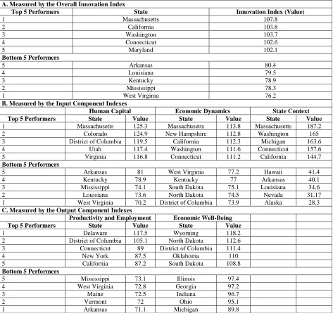
With respect to the Innovation Index as a whole, California, Connecticut, Massachusetts, Maryland, and Washington are the top 5 performers having Innovation Index values from 102.1 to 107.8. On the other hand, Arkansas, Kentucky, Louisiana, Mississippi, and West Virginia are the bottom 5 performers with Innovation Index values between 76.2 and 80.4 inclusive. A slightly different ranking can be seen with the component indexes (Appendix Table A2).
6. RESULTS AND DISCUSSION
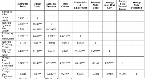
Table 2 shows the pairwise correlation among the variables used in this study. The average state per capita real GDP (from 1997 through 2011) is moderately correlated with Human Capital, highly correlated with Productivity & Employment, and minimally correlated with Economic Well-Being. These correlations are all statistically significant. On the other hand, the average state per capita personal income (from 1997 through 2011) is also moderately correlated with Human Capital, Economic Dynamics, State Context, and Productivity & Employment. These correlations are also statistically significant.
Table 2: Correlation among the Different Variables used in Regression Models
Innovation Index
Human Capital
Economic Dynamics
State Context
Productivity & Employment
Economic Well-Being
Average State Real
GDP
Average State Personal
Income
Average State Population
Innovation
Index 1
Human
Capital 0.9097*** 1
Economic
Dynamics 0.8069*** 0.6248*** 1
State
Context 0.7418*** 0.6809*** 0.6380*** 1
Productivity & Employment
0.6028*** 0.4058*** 0.2089 0.4425*** 1
Economic
Well-Being 0.1585 0.1519 -0.0084 -0.1953 0.0840 1
Average State Real GDP (per capita)
0.4769*** 0.4101*** 0.0718 0.2209 0.7246*** 0.2990** 1
Average State Personal Income (per capita)
0.7428*** 0.6345*** 0.5197*** 0.5022*** 0.6107*** 0.2168 0.7822*** 1
Average State Population
0.2216 0.1799 0.2913** 0.2407* 0.0786 -0.3055 -0.0438 0.1299 1
Asterisks *, **, and *** indicate significance at 10%, 5%, and 1% respectively.
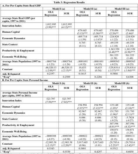
Table 3 shows the OLS and SUR regression results. They give identical regression coefficients, with only a very slight difference in the statistical significance of each coefficient between the two methods. Both average state per capita real GDP and per capita personal income are significantly positively associated with the overall Innovation Index (Model I (a) and Model I (b)) after controlling for the average state population (over 1997 through 2011). Consistent with the previous research (Wennekers & Thurik, 1999; Carree & Thurik, 2003), broadly speaking, the more innovative a state is (as measured by the value of the Innovation Index), the more productive it will be (measured in terms of the average state per capita real GDP) and the more income it can earn (measured in terms of the average state per capita personal income).
(Model III (b)). The coefficient of Human Capital in Model III (a) in Part A of Table 3 is 378.496 and significant across the OLS Regression and SUR. On the other hand, both the coefficients of Human Capital and Economic Dynamics in Model III (b) in Part B of Table 3 are significant and are 119.148 and 131.793 respectively. Hypothesis H1 (related to theimpact of Human Capital on per capita real GDP and/or per capita personal income) is thus fully supported whereas Hypothesis H2 (related to theimpact of Economic Dynamics on per capita real GDP and/or per capita personal income) is not as much. These results suggest that the more the population and labor of a state can engage in the state's innovative activities, the higher per capita real GDP can be generated by the state and the higher per capita personal income can be earned by its residents. At the same time, the better the local business conditions and the more resources available to its entrepreneurs and businesses of a state, the higher per capita personal income can be earned.
These findings imply that, in order to raise the overall living standard of the residents of a state, state policymakers should consider making more effort in and allocating more resources to several different areas. These should include, but are not limited to: (i) enhancing the state’s education system to offer more chances for the residents to receive higher education of greater variety so as to cultivate and expand their creativity and capability of forming innovative ideas, (ii) attracting and assisting more young people to move into (and/or to stay in) the state to work for the local existing businesses or establish, if possible, their own businesses, (iii) helping build and/or continue improve those innovative industries that can drive economic growth, and (iv) boosting employment by the high-tech firms. In addition, policymakers should also consider having some new incentives and/or enhancing those already in place to encourage more business R&D activities and venture capital investment in their state. One way to encourage R&D is to raise the tax credit businesses can receive on them. Perhaps the most effective way to bring in more (and/or retain the existing) venture capital is to lower or eliminate the existing, if any, capital gains tax rate. Capital gains tax here is in fact a tax on entrepreneurship. Furthermore, the state policymakers might consider enabling the state to commit funds in the out-of-state venture capital firms but requiring them to set up an establishment in the state. These should promote the flow of venture capital funds into the state and/or the stay of the funds within the state. At the same time, policymakers will also have to help strengthen the state’s infrastructure (for example, broadband density and transportation system). This should enable better connections between (i) businesses and their employees as well as (ii) businesses and their customers. Replacing firms in the outdated industries with firms in the new, emerging and innovative industries as well as encouraging and helping young people start their businesses (usually small for start-ups) are also something policymakers need to think about if their major objective is to improve the standard of living of the residents.
Table 3: Regression Results A. For Per Capita State Real GDP
Model I (a) Model II (a) Model III (a)
OLS
Regression SUR
OLS
Regression SUR
OLS
Regression SUR
Average State Real GDP (per capita, 1997 to 2011)
Innovation Index 1,012.995
(3.99)***
1,012.995 (4.12)***
Human Capital 679.645
(3.13)*** 679.645 (3.30)*** 378.496 (2.26)** 378.496 (2.44)*
Economic Dynamics -405.714
(-1.59) -405.714 (-1.67)* -224.820 (-1.22) -224.820 (-1.31)
State Context 8.765
(0.11) 8.765 (0.12) -69.339 (-1.10) -69.339 (-1.18)
Productivity & Employment 1,363.520
(6.48)***
1,363.520 (6.98)***
Economic Well-Being 501.555
(1.38)
501.555 (1.48) Average State Population (1997 to
2011) -.0003764 (-1.23) -.0003764 (-1.26) -.0001691 (-0.52) -.0001691 (-0.55) -.0000565 (-0.23) -.0000565 (-0.25)
Constant -46,520.13
(-2.08)** -46,520.13 (-2.15)** 10,433 (0.51) 10,433 (0.54) -129,818.4 (-3.57)*** -129,818.4 (-3.84)***
Adj. R-Squared 0.2197 0.1615 0.5804
"R-sq" 0.2509 0.2286 0.6308
B. For Per Capita State Personal Income
Model I (b) Model II (b) Model III (b)
OLS
Regression SUR
OLS
Regression SUR
OLS
Regression SUR
Average State Personal Income (per capita, 1997 to 2011)
Innovation Index 523.797
(7.59)***
523.797 (7.82)***
Human Capital 194.994
(2.97)*** 194.994 (3.12)*** 119.148 (1.95)* 119.148 (2.10)**
Economic Dynamics 92.967
(1.20) 92.967 (1.27) 131.793 (1.96)* 131.793 (2.11)**
State Context 8.886
(0.38) 8.886 (0.40) -5.782 (-0.25) -5.7824 (-0.27)
Productivity & Employment 307.596
(4.01)***
307.596 (4.32)***
Economic Well-Being 158.871
(1.20)
158.871 (1.29) Average State Population (1997 to
2011) -.0000308 (-0.37) -.0000308 (-0.38) -.000022 (-0.22) -.000022 (-0.23) .0000131 (0.15) .0000131 (0.16)
Constant -12,983.38
(-2.13)** -12,983.38 (-2.20)** 5,917.603 (0.96) 5,917.603 (1.01) -29,783.6 (-2.25)** -29,783.6 (-2.42)**
Adj. R-Squared 0.5343 0.3801 0.5512
"R-sq" 0.5530 0.4297 0.6050
t-statistics (z-scores) are shown in brackets beneath the OLS regression (SUR) coefficient. Asterisks *, **, and *** indicate significance at 10%, 5%, and 1% respectively.
7. CONCLUSION
personal income is associated with both the availability of human capital for innovative activities and the presence of the economic dynamics that facilitate those activities. At the same time, the higher per capita real GDP has been brought about by the availability of such human capital only. Other variables that are claimed to be theoretically important, such as those related to science and engineering graduates from state institutions, total R&D expenditures as a percentage of state GDP, included jointly in the State Context index, are not found significantly associated with either the per capita real GDP or the per capita personal income of the states.
AUTHOR INFORMATION
Oi Lin Cheung, Ph.D., is an Assistant Professor of Finance at Indiana University East. She has given numerous presentations regarding stock volatility transfers, market timing, and regulations in Dallas (Texas), Nashville (Tennessee), and Charleston (South Carolina). In 2006-2007, she received the Outstanding Ph.D. Student Toussaint Hocevar Award from the University of New Orleans. E-mail: ocheung@iue.edu
REFERENCES
1. Acs, Z., & Audretsch, D. (1989). Patents as a measure of innovative activity. Kyklos, 42(2), 71-81. 2. Agbetsiafa, D. (2010). Regional integration, trade openness, and economic growth: Causality evidence
from UEMOA countries. The International Business & Economics Research Journal, 9(10), 55-67. 3. Aghion, P., & Howitt, P. (1992). A model of growth through creative destruction. Econometrica, 60(2),
323-351.
4. Aghion, P., & Howitt, P. (1998). Endogenous growth theory. London: MIT Press.
5. Arora, V., & Vamvakidis, G. (2006). The impact of U.S. economic growth on the rest of the world: How much does it matter? Journal of Economic Integration, 21(1), 21-39.
6. Birch, D. (1987). Job creation in America: How our smallest companies put the most people to work. New York: Free Press.
7. Carree, M., & Thurik, R. (2003). The impact of entrepreneurship on economic growth. In D. Audretsch & Z. Acs (eds.), Handbook of entrepreneurship research (pp. 437-471). Boston/Dordrecht: Kluwer-Acadmic Publishers.
8. Carree, M., van Stel, A., Thurik R., & Wennekers, S. (2002). Economic development and business ownership: An analysis using data of 23 OECD countries in the period 1976-1996. Small Business Economics, 19, 271-290.
9. Coe, D., & Helpman, E. (1995). International R&D spillovers. European Economic Review, 39, 859-887. 10. Crosby, M. (2000). Patents, innovation and growth. Economic Record, 76(234), 255-262.
11. Cebula, R., Clark, J., & Mixon, F. (2013). The impact of economic freedom on per capita real GDP: A study of OECD nations. Journal of Regional Analysis & Policy, 43(1), 34-41.
12. Dawson, J. (1998). Institutions, investment, and growth: New cross-country and panel data evidence. Economic Inquiry, 36(4), 603-619.
13. Denison, E. (1962). The sources of economic growth in the states and the alternatives before us. New York: Committee for Economic Development.
14. Engelbrecht, H. (1997). International R&D spillovers amongst OECD economies. Applied Economics Letters, 4, 315-319.
15. Feldman, M. (2005). Chapter 2: The significance of innovation. In G. Hallen & A. Osthol (ed.), The growth policy agenda. Swedish Institute for Growth Policy Studies (in English and Swedish).
16. Gani, A., & Clemes, M. (2002). Services and economic growth in ASEAN economies. ASEAN Economic Bulletin, 19(2), 155-169.
17. Griliches, Z. (1990). Patent statistics as economic indicators: A survey. Journal of Economic Literature, 28, 1661-1707.
18. Grossman, G., & Helpman, E. (1991). Innovation and growth in the global economy. Cambridge, MA: MIT Press.
20. Guellec, D., & van Pottelsberghe de la Potterie, B. (2001). R&D and productivity growth: Panel data analysis of 16 OECD countries. (STI Working Paper 2001/3). Directorate for Science, Technology and Industry, OECD, Geneva.
21. Indiana Business Research Center. (n.d.). Innovation index methodology. Retrieved from http://www.statsamerica.org/innovation/innovation_index/methodology.html
22. Indiana Business Research Center. (2009). Crossing the next regional frontier: Information and analytics linking regional competitiveness to investment in a knowledge-based economy. Retrieved from
http://www.statsamerica.org/innovation/report_next_regional_frontier_2009.html
23. Hall, B. (2007). Patents and patent policy. Oxford Review of Economic Policy, 23, 568-87.
24. Jones, C. (2002). Sources of US economic growth in a world of ideas. American Economic Review, 92(1), 220-39.
25. Jorgenson, D., & Griliches, Z. (1967). The explanation of productivity change. Review of Economic Studies, 34, 249-84.
26. Kremer, M. (1993). Population growth and technological change: One million B.C. to 1990. Quarterly Journal of Economics, 108(3), 681-716.
27. Kumah, F., & Sandy, M. (2013). In search of inclusive growth: The role of economic institutions and policy. Modern Economy, 4(11), 758-775.
28. Lichtenberg, F. (1993). R&D Investment and international productivity differences. (NBER Working Paper No. 4161).
29. Lucas, R. Jr. (1988). On the mechanics of economic development. Journal of Monetary Economics, 22, 3-42.
30. Mansfield, E. (1972). Contribution of research and development to economic growth of the United States. Papers and Proceeding of a Colloguim on Research and Development and Economic Growth Productivity. National Science Foundation, Washington DC.
31. Malchow-møller, N., Schjerning, B., & Sørensen, A. (2011). Entrepreneurship, job creation and wage growth. Small Business Economics, 36(1), 15-32.
32. Nadiri, M. (1993). Innovations and technological spillovers. (NBER Working Paper, No. 4423). 33. Neumark, D., Zhang, J., & Wall, B. (2006). Where the jobs are: Business dynamics and employment
growth. Academy of Management Perspectives, 20, 79-94.
34. Neumark, D., Wall, B., & Zhang, J. (2008). Do small businesses create more jobs? New evidence from the national establishment time series. (NBER working paper no. 13818). National Bureau of Economic Research (NBER), Cambridge.
35. Pack, H. (1994). Endogenous growth theory: Intellectual appeal and empirical shortcomings. Journal of Economic Perspectives, 8(1), 55-72.
36. Porter, M. (1996). What is strategy? Harvard Business Review, 74(6), 61.
37. Romer, P. (1986). Increasing returns and long run growth. Journal of Political Economy, 94(5), 1002-1037. 38. Romer, P. (1990). Endogenous technological change. Journal of Political Economy, 98, 71-102.
39. Ruttan, V. (1997). Induced innovation, evolutionary theory and path dependence: Sources of technical change. Economic Journal, 107, 1520-1529.
40. Schumpeter, J. (1911). The theory of economic development. Cambridge, MA: Harvard University Press. 41. Schumpeter, J. (1934). Theory of economic development (1911, in German; tr. 1934). Cambridge, MA:
Harvard University Press.
42. Schumpeter, J. (1939). Business cycles: A theoretical, historical and statistical analysis of the capitalist process, 2 volumes. New York: McGraw-Hill.
43. Schumpeter, J. (1942). Capitalism, socialism, and democracy. New York: Harper & Row 1976 edition. 44. Sedgley, N. (2006). A time series test of innovation-driven endogenous growth. Economic Inquiry, 44(2),
318-332.
45. Slaper, T., & Justis, R. (2010). Measuring regional capacity for innovation. Incontext, 11(1). Retrieved from http://www.incontext.indiana.edu/2010/jan-feb/article1.asp
46. Smith, A. (1776). An inquiry into the nature and causes of the wealth of nations. Modern Library edition, NY, NY, 1937.
48. Solow, R. (1957). Technical change and the aggregate production function. Review of Economics and Statistics, 312-320.
49. Torun, H., & Çiçekci, H. (2007). Innovation: Is the engine for the economic growth. The Faculty of Economics and Administrative Sciences, Ego University, Izmir.
50. Verspagen, B. (1992). Endogenous innovation in neo-classical growth models: A survey. Journal of Macaroeconomics, 14, 631-662.
51. Wennekers S., & Thurik, R. (1999). Linking entrepreneurship and economic growth. Small Business Economics, 13(1), 27-55.
APPENDIX
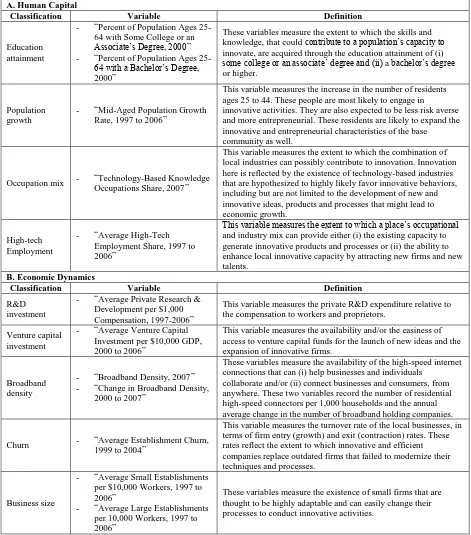
Table A1: Definitions of the Variables Used in the Computation of the Component Indexes of the Innovation Index (Indiana Business Research Center, 2009)
A. Human Capital
Classification Variable Definition
Education attainment
- “Percent of Population Ages 25-64 with Some College or an Associate’s Degree, 2000” - “Percent of Population Ages
25-64 with a Bachelor’s Degree, 2000”
These variables measure the extent to which the skills and knowledge, that could contribute to a population’s capacity to innovate, are acquired through the education attainment of (i) some college or an associate’ degree and (ii) a bachelor’s degree or higher.
Population growth
- “Mid-Aged Population Growth Rate, 1997 to 2006”
This variable measures the increase in the number of residents ages 25 to 44. These people are most likely to engage in
innovative activities. They are also expected to be less risk averse and more entrepreneurial. These residents are likely to expand the innovative and entrepreneurial characteristics of the base community as well.
Occupation mix - “Technology-Based Knowledge Occupations Share, 2007”
This variable measures the extent to which the combination of local industries can possibly contribute to innovation. Innovation here is reflected by the existence of technology-based industries that are hypothesized to highly likely favor innovative behaviors, including but are not limited to the development of new and innovative ideas, products and processes that might lead to economic growth.
High-tech Employment
- “Average High-Tech Employment Share, 1997 to 2006”
This variable measures the extent to which a place’s occupational and industry mix can provide either (i) the existing capacity to generate innovative products and processes or (ii) the ability to enhance local innovative capacity by attracting new firms and new talents.
B. Economic Dynamics
Classification Variable Definition
R&D investment
- “Average Private Research & Development per $1,000 Compensation, 1997-2006”
This variable measures the private R&D expenditure relative to the compensation to workers and proprietors.
Venture capital investment
- “Average Venture Capital Investment per $10,000 GDP, 2000 to 2006”
This variable measures the availability and/or the easiness of access to venture capital funds for the launch of new ideas and the expansion of innovative firms.
Broadband density
- “Broadband Density, 2007” - “Change in Broadband Density,
2000 to 2007”
These variables measure the availability of the high-speed internet connections that can (i) help businesses and individuals
collaborate and/or (ii) connect businesses and consumers, from anywhere. These two variables record the number of residential high-speed connectors per 1,000 households and the annual average change in the number of broadband holding companies.
Churn - “Average Establishment Churn, 1999 to 2004”
This variable measures the turnover rate of the local businesses, in terms of firm entry (growth) and exit (contraction) rates. These rates reflect the extent to which innovative and efficient companies replace outdated firms that failed to modernize their techniques and processes.
Business size
- “Average Small Establishments per $10,000 Workers, 1997 to 2006”
- “Average Large Establishments per 10,000 Workers, 1997 to 2006”
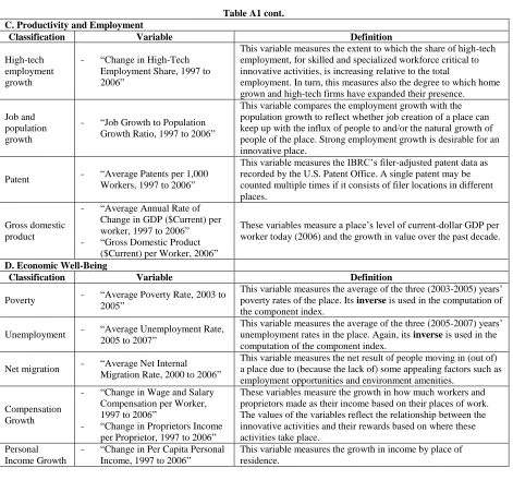
Table A1 cont. C. Productivity and Employment
Classification Variable Definition
High-tech employment growth
- “Change in High-Tech Employment Share, 1997 to 2006”
This variable measures the extent to which the share of high-tech employment, for skilled and specialized workforce critical to innovative activities, is increasing relative to the total
employment. In turn, this measures also the degree to which home grown and high-tech firms have expanded their presence.
Job and population growth
- “Job Growth to Population Growth Ratio, 1997 to 2006”
This variable compares the employment growth with the population growth to reflect whether job creation of a place can keep up with the influx of people to and/or the natural growth of people of the place. Strong employment growth is desirable for an innovative place.
Patent - “Average Patents per 1,000 Workers, 1997 to 2006”
This variable measures the IBRC’s filer-adjusted patent data as recorded by the U.S. Patent Office. A single patent may be counted multiple times if it consists of filer locations in different places.
Gross domestic product
- “Average Annual Rate of Change in GDP ($Current) per worker, 1997 to 2006” - “Gross Domestic Product
($Current) per Worker, 2006”
These variables measure a place’s level of current-dollar GDP per worker today (2006) and the growth in value over the past decade.
D. Economic Well-Being
Classification Variable Definition
Poverty - “Average Poverty Rate, 2003 to 2005”
This variable measures the average of the three (2003-2005) years’ poverty rates of the place. Its inverse is used in the computation of the component index.
Unemployment - “Average Unemployment Rate, 2005 to 2007”
This variable measures the average of the three (2005-2007) years’ unemployment rates in the place. Again, its inverse is used in the computation of the component index.
Net migration - “Average Net Internal Migration Rate, 2000 to 2006”
This variable measures the net result of people moving in (out of) a place due to (because the lack of) some appealing factors such as employment opportunities and environment amenities.
Compensation Growth
- “Change in Wage and Salary Compensation per Worker, 1997 to 2006”
- “Change in Proprietors Income per Proprietor, 1997 to 2006”
These variables measure the growth in how much workers and proprietors made as their income based on their places of work. The values of the variables reflect the relationship between the innovative activities and their rewards based on where these activities take place.
Personal Income Growth
- “Change in Per Capita Personal Income, 1997 to 2006”
Table A2: The Top and Bottom Five Innovative States A. Measured by the Overall Innovation Index
Top 5 Performers State Innovation Index (Value)
1 Massachusetts 107.8
2 California 103.8
3 Washington 103.7
4 Connecticut 102.6
5 Maryland 102.1
Bottom 5 Performers
5 Arkansas 80.4
4 Louisiana 79.5
3 Kentucky 78.9
2 Mississippi 78.3
1 West Virginia 76.2
B. Measured by the Input Component Indexes
Human Capital Economic Dynamics State Context
Top 5 Performers State Value State Value State Value
1 Massachusetts 125.3 Massachusetts 113.8 Massachusetts 187.2
2 Colorado 124.9 New Hampshire 112.8 Washington 165
3 District of Columbia 119.5 California 112.3 Michigan 163.6
4 Utah 117.4 Washington 111.6 Connecticut 157.6
5 Virginia 116.8 Connecticut 111.2 California 144.7
Bottom 5 Performers
5 Arkansas 81 West Virginia 77.2 Hawaii 41.4
4 Kentucky 78.9 Kentucky 77 Arkansas 40.1
3 Mississippi 74.1 South Dakota 75.1 Louisiana 34.6
2 Louisiana 73.6 North Dakota 74.5 Nevada 31.17
1 West Virginia 70.2 District of Columbia 73.9 Alaska 28.3
C. Measured by the Output Component Indexes
Productivity and Employment Economic Well-Being
Top 5 Performers State Value State Value
1 Delaware 117.5 Wyoming 118.2
2 District of Columbia 105.1 North Dakota 112.6
3 Connecticut 89 District of Columbia 111.4
4 New York 87.5 Oklahoma 110
5 California 87.2 South Dakota 108.8
Bottom 5 Performers
5 Mississippi 73.1 Illinois 97.4
4 West Virginia 72.8 Georgia 97.2
3 Maine 72.5 Indiana 96.7
2 Vermont 72 Ohio 95.1
1 Arkansas 71.1 Michigan 89.8