THE GLOBAL FINANCIAL CRISIS: AN ANALYSIS OF CONTAGION EFFECTS TO SELECTED MENA COUNTRIES

(1)

Licensed under Creative Common Page 142

http://ijecm.co.uk/

ISSN 2348 0386

THE GLOBAL FINANCIAL CRISIS: AN ANALYSIS OF

CONTAGION EFFECTS TO SELECTED MENA COUNTRIES

Lotfi Trabelsi

Assistant Professor of Finance,

Institute of the High Commercial Studies of Sfax-Tunisia (IHEC-Sfax), Tunisia [email protected]

Abstract

The incidence of ﬁnancial crises over the past decade has ignited research into the nature of the

spread of financial crises across borders, with the conduit of ‘contagion’ an important focus. Contagion is defined as an increase of common movements in a set of financial asset markets

in a particular period of time (a crisis period) compared to those existing in a benchmark

(non-crisis) period. The aim of this paper is to investigate the contagion effects from US to five MENA

stock markets namely, Bahrain, Kuwait, Egypt, Morocco and Tunisia before and during global

financial crisis (2007-2009). The methodology is based on the vector autoregressive regression

(VAR) model and the Granger causality test. Results show a "pure contagion" phenomenon

between some markets during the 2008 financial crisis. Furthermore, the causality effect is more

pronounced in crisis than calm period.

Keywords: Financial Crisis, MENA Countries, Contagion, Correlation, Causality

INTRODUCTION

(2)

Licensed under Creative Common Page 143 phenomenon of transmission of these crises from one country to another, and more specifically of financial market to another. This is often called "contagion." Indeed, several studies have been presented, which aims to investigate the causes and failures at the origin of this phenomenon. There is no unanimously accepted definition of financial contagion. The World Bank summarizes three layers within contagion definitions. In a broad sense, contagion is the cross-country transmission of shocks or general cross-country spillover effects. In a restrictive sense, contagion is the transmission of shocks to other countries, or cross-country correlation, beyond any fundamental link among the countries and beyond common shocks. In a very restrictive sense, contagion refers to an increase in cross-country correlations during “crisis times” relative to correlations during “tranquil times”. The very restrictive definition is commonly

used in recent empirical analysis to identify and measure financial contagion (Dungey et al., 2005; Forbes and Rigobon, 2002, among others). This paper follows this convention as defended by Kenourgios and Dimitriou (2015).

The objective in this paper is to highlight, through both co-integration within the meaning of Johansen (1988) and Granger causality (1969) tests, the changes in the causal relationship between the United States and five MENA countries, namely Bahrain, Kuwait, Egypt, Morocco and Tunisia over the period 2005 - 2009 . The presence of the "pure contagion" phenomenon is studied under the assumption of multiple equilibrium of Masson (1998), which assumes that the transmission of the crisis is through changes in investors' expectations, in that the transmission mechanisms during the crisis are different from those of the quiet period.

A multitude of empirical works used the purpose of detection of contagion, the foreign exchange markets, interest rates and sovereign debt. However, other authors have used the stock market as an indicator of expectations and behavior of international investors, to test the existence of contagion. In our study, we will proceed to the study of the behavior of co-movement between the stock markets.

The remainder of the paper is structured as follows. Section 2 reviews the literature on financial contagion; section 3 presents the dataset and introduces the methodology framework, while section 4 produces empirical estimation results and robustness tests. Finally, section 5 summarizes the findings and concludes.

LITERATURE REVIEW

(3)

Licensed under Creative Common Page 144 the multitude of advanced work was the subject of a strong controversy about the speed of its dissemination and geographic reach.

The study of the "subprime" crisis was the subject of a rather rich debate in order to reveal the causes and origins. In fact, the majority of work on this subject argue that this crisis started by the swelling of economic bubbles and losses of financial institutions caused by the securitized loans and has increased with the collapse of multiple financial leader organizations causing the start of a systemic crisis.

However, the originality of this crisis lies in a global crisis of confidence that was the major factor ensuring the deterioration of the global financial kingdom that has developed and grown with the adoption of the strategy of financial globalization and full liberalization of capital, which has put forward the concerns for the contagion, which has led researchers within the community of economists to reconcile theory with economic reality in order to provide relevant explanations to this phenomenon.

Because the world is becoming more and more economically and socially integrated and simultaneous crises becomes more intense, all these factors have led to the promotion of the concept of contagion. To understand it, we must clarify these propagation mechanisms. So the answer to the question is still very important: is the links between the countries are already intensified or become intense during the crisis? Indeed, this meaning is demonstrated in the work of Forbes and Rigobon (2000). They have two opposite theories in which they have developed mechanisms on interdependence and contagion concept, namely contingent theories crisis and non-crisis contingent theories:

 The non-contingent theories crises occur if the transmission mechanisms after the crisis are

not significantly different from those existing during the pre-crisis period. Indeed, in this case the crisis spread through trade links, financial and political ties between the countries.

 Contingent theories crisis operate on the principle that the propagation mechanisms change

significantly during crisis periods during which the behavior and anticipation of investors produce a leading role. In this context the crisis causes a structural change such that the shocks are propagated through a channel that does not exist during the period of financial stability.

(4)

Licensed under Creative Common Page 145  If the crisis spreads through not quotas channels to crises, so the monetary authorities can

not apply short term strategies as the crisis is the result of a long-term interdependent relationship.

 If the crisis spreads through quotas channels to crises, so, the monetary authorities may

mediate by applying short-term isolation strategies, for example by the application of capital controls.

The initial empirical literature on financial crisis and contagion focused on fundamentals-based mechanisms and was directed towards developing early warning systems (Eichengreen et al., 1996; Kaminsky et al., 1998; van Rijckghem and Weder, 2001), while later empirical works focused on investor behavior-based mechanisms (Bekaert et al., 2011; Dungey et al., 2005).

In a seminal paper, Forbes and Rigobon (2002) provide a breakthrough on the conventional correlation analysis approach for testing contagion. As volatility increases during a crisis, an increase in correlation may simply be a continuation of strong transmission mechanisms that exist in more stable periods. Forbes and Rigobon (2002) offer an adjusted correlation approach to test for contagion in 28 stock markets and three episodes of crisis. They conclude that the observed increase in correlation during crisis periods is due to increased interdependence among the markets, not contagion.

In slightly different fashion, Bekaert et al. (2005), Corsetti et al. (2005) and Dungey and Martin (2001), among others, follow a factor model of correlation analysis to test for contagion during different episodes of financial crisis.

We will explain in the following contagion theories presenting in the first part of the non-contingent theories crises and in second part non-contingent theories to crisis.

The "subprime" crisis was triggered in August 2007. It presents the most tragic crisis in American history since 1929. The occurrence of this crisis was in part the result of the stock market crash occurred in the United States in 2000 following the bursting of the Internet bubble. The immediate consequence of this crash was catastrophic in the sense that it has led to any US economic recession. In order to limit the damage from this situation, the US Federal Reserve decided in 2001 to provide liquidity to the market. At the same time, lower interest rates is decided not to be too slow consumer spending and investment, and therefore not to hinder growth. The impact of these decisions the Fed did not wait in the sense that economic agents and households in particular have begun to invest heavily in real estate, which resulted in the sharp increase in appropriations mortgages and house prices.

(5)

Licensed under Creative Common Page 146 and prevent the spread of these effects to other countries of the world by the massive injection of liquidity, the US crisis was transmitted in proportions variables, other countries around the world in less than two years.

After studying several works, we can conclude that this crisis affects all economic components systems, not just the mortgage sector. The intensity of the crisis and the extent of damages granted to it, have allowed researchers to raise formidable questions regarding:  The advantages and disadvantages of securitization procedures,

 The role of financial innovations in risk transfer,

 The internal risk control and the actual organization of prudential supervision systems and

banking supervision,

 The general system of banking and financial regulation.

METHODOLOGY

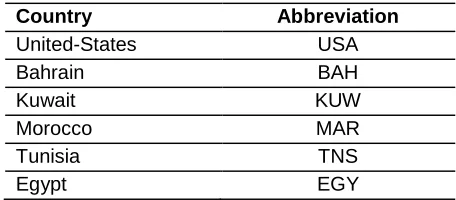
Daily closing prices of stock market index from 6 countries are examined in this study. We consider the following 6 countries: Bahrain (BAH), Kuwait (KUW), Morocco (MAR), Egypt (EGY), Tunisia (TNS) and United States (USA). Furthermore, to investigate the "pure contagion" of stock markets in the USA, we will base our analysis on the price of the US stock market index S&P500. All indexes are denominated in US dollars. This allows us to capture the behavior of international investors. Our sample period covers June 1, 2005 to September 1, 2009. The quiet period, begin June1, 2005 and end June 29, 2007. For the crisis period we chose, as several studies, the period from July 2, 2007 to September 1, 2009. We therefore consider that the date of onset of the crisis is July 2, 2007, by referring to luliana Matei (2010). All data are from the MSCI database.

Table 1: Series Abbreviations

Country Abbreviation

United-States USA

Bahrain BAH

Kuwait KUW

Morocco MAR

Tunisia TNS

Egypt EGY

Correlations Study

(6)

Licensed under Creative Common Page 147 effect of the change in the market volatility originating from a crisis, which causes heteroscedasticity. To correct this bias, an adjustment is required. Therefore, we use the one proposed by Forbes and Rigobon (2001).

t X

andYt_{are two financial series identifying the index returns in two different markets. To} examine the relationship between the returns in different markets, we make use of the simple

linear model as follows: Yt 







Xt 



t_{with, E (}



t_{)=0, E(}



t_{²) <}



_E(Xt



t_)=0, The correlation coefficient between the two series can be measured by:









t t y x t t t

t x y

y x





, cov ,

.

The adjusted correlation coefficient proposed by Forbes and Rigobon (2002) is then

*



such as:



 



2 *

1

1 









. With

 



1 

t t t c

x

V

x

V



Where "c" and "t" indicate the crisis and the quiet periods

Indeed,



represents the relative increase in the variance of x between the two periods.

After calculating the adjusted correlation coefficient for each pair of countries in the sample, we will statistically test its increase during the crisis period, to make sure that there is a pure contagion or not. Thus, to statistically test the rise of an adjusted correlation coefficient, we will use the following two alternative hypotheses:

* 2 * 1 1 * 2 * 1 0

:







H

With, * 1

 _{: The correlation coefficient of the crisis period.}

* 2



_{: The correlation coefficient of the quiet period.}

To test these hypotheses, we use a Student's test used by Collins and Biekpe (2002) whose statistics is:



_{ }

_*

_

2

2 * 1 2 1 * 2 * 1 1 4



    

 n n

t

, with, t indicates a Student to (

n

1



n

2



4

_{) degrees of freedom.}

(7)

Causality Study

To conduct a causality study, we must make the first step in testing stationarity. If we find that the series are non-stationary at the same level, we proceed to test for co-integration. Two cases can be distinguished depending on whether the series are co-integrated or not. In the absence of co-integration, we must estimate a VAR in first difference because the variables are integrated of order 1 and causality tests are applied to the series in first difference. Besides, in case of existence of co-integration relationships, an error correction term must be introduced into the VAR model of order K which becomes a VECM of order K-1, and in the latter case there are two types of causation tests: a short-term causality and a long-term causality.

In what follows, we will test the stationarity of the series of the index returns via the ADF and Phillips-Perron tests for two sub-periods (stability and crisis). Then, we will identify the number of co-integrating relationships for each of the two sub-periods, before studying the evolution of the causal links between the quiet and the crisis periods.

Stationarity Tests

To test the presence of unit root in the series, we will apply the Augmented Dickey-Fuller test (ADF test) and Phillips Perron’s test.

The ADF test considers three basic models for a single series (Xt where t = 1,… T):

 a model without constant or deterministic trend  a model with constant and without deterministic trend  a model with constant and deterministic trend.

The ADF tests the null hypothesis of the presence of unit root (the series Xt is non-stationary

i.eXt Integrated of order 1) against the alternative hypothesis of no unit root (the series Xt is

stationary i.e integrated of order 0). Regression refers to the ADF test can be written as follows:

t t i k i t

t X X

X 











 



 _₁ _₁ _₁ ₍₁₎

 The null hypothesis



= 0 implies that the series Xt is non-stationary in level.

 The alternative hypothesis



<0 implies the absence of a unit root.

It should be noted that if the series is non-stationary under the null hypothesis, the test statisticwill have a non-standard distribution and the lag order k is determined, for each series, by the method of criteria information. The latter consists in selecting among a number of models estimated for a number of lag from 0 to h (h is the maximum lag) one whose lag (p) minimizes the Akaike criteria (AIC) and Schwarz (SC) defined as follows:



N P T



(8)



T T



p N

SClogdet^  2 log /



Where,

N is the number of variables, T is the number of observations and  is an estimator of the variance-covariance matrix of residuals.

The test is applied first on the level series following a sequential strategy to identify an appropriate model. In the case where the series is non-stationary in level, we will apply the test on first difference series. The application of the Phillips-Perron test is identical to that of Dickey-Fuller, except that it requires the choice beforehand of parameter truncation (l) intervened in the calculation of the long term variance of the residuals. We will than present, for each variable, the results obtained with the value suggested by Newey and West (1987): l = int [4 (T/100) 2/9].

Johansen Co-integration Tests

Co-integration refers to the presence of long-term stable relationships between the variables Xt

and Yt. To determine the number of co-integration relationships, Johansen developed two

statistics: the trace statistics and the maximum eigen value statistics. These two statistics coincide in their null hypotheses, but differ in their alternative hypotheses:

The trace statistics tests on a co-integrated VAR:

 The null hypothesis: there are at most r co-integrating relationships between X and Y

 The alternative hypothesis: there are at least r + 1 co-integrating relations between X and Y.

The maximum eigen value test Statistics:

 The null hypothesis: there are at most r co-integrating relationships between the variables X

and Y.

 The alternative hypothesis: there are exactly r + 1 co-integrating relations between X and Y.

Proceeding with tests of ADF and PP, we demonstrated that all series are integrated of order 1. We therefore have the right to pass the tests of integration. To determine the number of co-integrated vectors, we use the trace test which is more powerful than that of the maximum eigen value (Matei 2010).

Granger Causality Tests

According to Lardic and Mignon (2002), variable X causes variable Y in the Granger sense if and only if knowledge of the past of X improves the prediction of Y. Non-Granger causality means that the past of variable Xt provides no additional information to variable Yt. Non-causality is showed using a test of significance of the Xt coefficient delays in a regression of Yt

(9)

Licensed under Creative Common Page 150 coefficients of Xt delays are significantly different from zero. In our work, both variables Xt and

Yt represent the series of the index returns of two countries. We follow the methodology of Sander and Kleimeier (2003) and consider the bivariate VAR model in levels as follows:

t x t i x t

i x x

t X Y

X 







_, ₁



_, ₁



_, _{(2) (causality of Y to X)}

t y t i y t

i y y

t Y Y

Y 







, 1



, 1



, _{(3) (causality of X to Y)}

The Granger causality therefore tests if all the coefficients



i_{are zero with a standard test (F).} Three possibilities can be identified at this level:

 If we reject H0 (



x_{= 0) in equation (2), we can say that Y causes X in the Granger sense.}

 If we reject H0 (y_{= 0) in equation (3), we can say that X causes Y in the Granger sense.}

 If we reject the null hypothesis of no causality in the two previous cases, variables X and Y

are therefore interdependent.

Before performing the tests of Granger causality, we have to estimate VECM and VAR models through which we will test causality. Two cases can be distinguished depending on whether the series are co-integrated or not: In the absence of co-integration relationships, we estimate a VAR in first differences because the variables are integrated of order 1 and the tests of Granger causality will be applied to the series in first difference. If there is a co-integration relationship between variables X and Y, an error correction term must be introduced into the VAR model in difference. The VAR model of order k becomes a VECM of order (k-1) as follows:

t x t x x t i x t

i x x

t X Y ECT

X 







, 1



, 1



, 1



,

 _ _ _

(4)

t y t y y t i y t

i y y

t Y X ECT

Y 







, 1



, 1



, 1



,

 _ _ _

(5) ECT : the term error correction

In the case of a VECM, there are two types of causality to be tested: a non-causality of short term of Y on X and a non-causality of long-term of Y on X. The order of the VAR or VECM is determined by the information criteria method and based primarily on criteria of Akaike (AIC) and Schawrtz (SIC). When these two criteria diverge, we will opt for the first test since it is considered an efficient estimator of p (Lardic and Mignon (2002)).

(10)

EMPIRICAL RESULTS

Descriptive Analysis

The preliminary study of the series, aims to study their steady states as based on the graphic representations, and to analyze the descriptive statistics, ultimately, to the study of correlations between the different variables.

Graphical Analysis

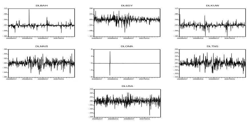
The evolution of stock index returns of each country in the sample is given by the graphs in Figure 1 and 2 in the appendices. The graphs show a significant simultaneous collapse of indexes from July 2007, the triggering date of the crisis of the subprime mortgages in the United States. This collapse became even more serious as soon as the beginning of 2008. This graphical analysis is supported further by descriptive statistics forming the subject of the next section.

Descriptive Statistics

Referring to the results given in table 2 in appendices, we can conclude that the hypothesis of normality is rejected seen the values of skewness being different from 0 and kurtosis different from 3 and in addition, the Statistic of Jarque-Bera is, in all cases, sufficiently greater than 5.99. In this case, we can assume that series are characterized by the presence of heteroscedasticity. From table 3 in appendices, we note that the average has increased by 3.5% during the crisis period, except in the case of Bahrain and the United States where it marked a fall of 25%.

Following these results, we can observe that the US, Bahrain and Kuwait are the most affected countries by the crisis to the decrease in their average (except Kuwait) and the remarkable increase their volatility, and Tunisia and Morocco are the countries affected ways to increase their average and reduced their volatility during the crisis.

Adjusted Correlation Coefficient Tests

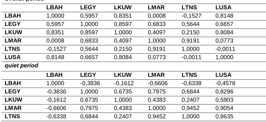
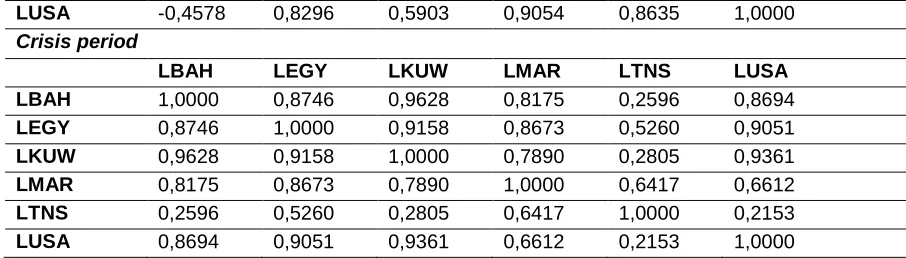
The Correlation study provides a preliminary description of the relationship between the various parities market indexes. This study based on the two sub-periods allows us to have an idea about their evolution. Table 4 in appendices shows the correlation matrices of the overall period and the two sub-periods. From table 4, correlations in overall period bring up two groups of strong correlations:

(11)

Licensed under Creative Common Page 152 between this period and the quiet period. For this latter, most of the correlation values are negative.

- The second group incorporates Tunisia and Morocco, where the brand is stronger. Correlation value equal to 0.9191. Unlike the first group these values are essentially explained during the quiet period. We can note that their correlation values with other countries are too low, except in the case of Egypt being 0.5644 and 0.6833, respectively. We also note that the correlations between Marocoo-United States and Tunisia-United States have increased significantly during the quiet period relative to the overall period of crisis.

Regarding the evolution of the correlations of the quiet and the crisis periods between the studied countries and the United States, we can conclude that all values have increased, except Tunisia and Morocco where represents a decrease in these values.

Following these results, we can confirm the findings from the survey of the mean and volatility. Indeed, we can affirm that it seems to have evidence of "subprime" contagion to Bahrain, Kuwait and Egypt but not in the case of Tunisia and Morocco.

Through this descriptive study, we could make a preliminary idea on stationary and on the evidence of correlation coefficient test, so it would be legitimate to confirm these insights by studying the Granger causality.

Stationarity Tests

The application of the Augmented dickey Fuller (ADF) test (table 5 in the appendices) reveals that all studied series are integrated in order one I(1), either for quiet period or for the crisis period, with reserve in case of Bahrain throughout the crisis period since it is I(1) only at a confidence level of 1%. Indeed, applying the ADF test on the series in first differences, we find that the series is I(0) has a confidence level of 1% and 5%, then the series of Bahrain is I(1).

To ensure more robustness to the study of stationarity, we propose to apply in addition to the ADF test, the Phillips-Perron (PP) test. Phillips and Perron(1988) suggest, in fact, a non-parametric correction Dickey-Fuller test to solve the problem of correlation and/or heteroscedasticity.

The results of PP test confirm those from the ADF test. Indeed, all the studied series are integrated in order 1 for the two study periods (table 6 in the appendices).

(12)

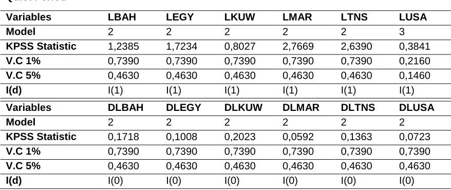
Licensed under Creative Common Page 153 The results of the KPSS test (table 7 in the appendices) confirm the results from both ADF and PP tests, with reserve in the case of Bahrain during the crisis. Indeed, the series of Bahrain is I (2). In this case, taking into account the results of the three tests, we consider this set as I (1).

Referring to the results of the three tests, we can conclude that all studied series are integrated in order 1 either during the quiet or the crisis period. These results are consistent with results from the graphic study presented above in the preliminary analysis.

Johansen Co-Integration Tests

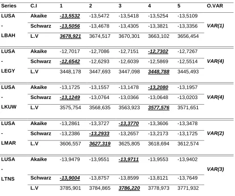
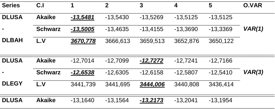
As shown in the previous sections, the study of co-integration is only possible if the two series are integrated in order 1. The procedure of Johansen is thus applied on non-stationary series level. To determine the number of co-integrated vectors, we applied the track test and the eigen value test. Before performing the co-integration test, it is essential to choose the order of the VAR (using the series level) for each pair of countries and each sub-period using information criteria (tables). The recapitulation of the two tables 8 and 9 (in the appendices) is presented in table 12

Table 12: Order of VAR for both periods

Series Order of VAR for quiet period Order of VAR for crisis period

LUSA – LBAH VAR(1) VAR(3)

LUSA – LEGY VAR(4) VAR(5)

LUSA – LKUW VAR(4) VAR(1)

LUSA – LMAR VAR(2) VAR(3)

LUSA – LTNS VAR(3) VAR(2)

Co-integration tests are conducted separately on the quiet and the crisis periods. The following tables present a summary of our results:

Table 13: Co-integration test (quiet period)

Country Eigenvalues T. prob

V.P

Trace T. prob

Trace

Co-integration

Tstat Tcrit 5% Tstat Tcrit 5%

USA - BAH

r=0 7.2027

r=1 0.2746

r=0 14.2646

r=1 3.8414

r=0 0.4654

r=1 0.6002

r=0 7.4774

r=1 0.2746

r=0 15.4947

r=1 3.8414

r=0 0.5228

r=1 0.6002

NO

USA - EGY

r=0 9.2701

r=1 0.2950

r=0 14.2646

r=1 3.8414

r=0 0.2644

r=1 0.5870

r=0 9.5652

r=1 0.2950

r=0 15.4947

r=1 3.8414

r=0 0.3157

r=1 0.5870

(13)

Licensed under Creative Common Page 154 USA - KWT r=0 2.9674 r=1 0.0107 r=0 14.2646 r=1 3.8414 r=0 0.9489 r=1 0.9173 r=0 2.9781 r=1 0.0107 r=0 15.4947 r=1 3.8414 r=0 0.9679 r=1 0.9173 NO USA - MAR r=0 7.1384 r=1 0.2766 r=0 14.2646 r=1 3.8414 r=0 0.4729 r=1 0.5989 r=0 7.4151 r=1 0.2766 r=0 15.4947 r=1 3.8414 r=0 0.5299 r=1 0.5989 NO USA - TNS r=0 2.7095 r=1 0.4054 r=0 14.2646 r=1 3.8414 r=0 0.9642 r=1 0.5243 r=0 3.1149 r=1 0.4054 r=0 15.4947 r=1 3.8414 r=0 0.9615 r=1 0.5243 NO

The decision rule for this test is to reject the null hypothesis of r co-integrating relationship: when TR statistics is greater than its critical value and the same for eigen value statistics.

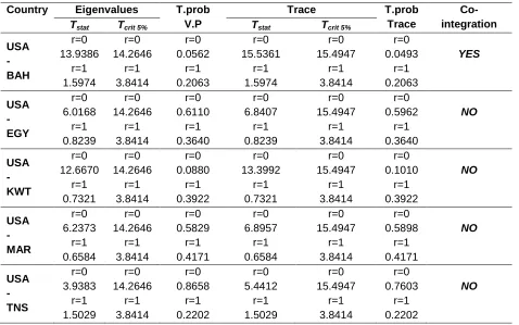
Table 14: Co-integration Test (Crisis Period)

Country Eigenvalues T.prob

V.P

Trace T.prob

Trace

Co-integration

Tstat Tcrit 5% Tstat Tcrit 5%

USA - BAH r=0 13.9386 r=1 1.5974 r=0 14.2646 r=1 3.8414 r=0 0.0562 r=1 0.2063 r=0 15.5361 r=1 1.5974 r=0 15.4947 r=1 3.8414 r=0 0.0493 r=1 0.2063 YES USA - EGY r=0 6.0168 r=1 0.8239 r=0 14.2646 r=1 3.8414 r=0 0.6110 r=1 0.3640 r=0 6.8407 r=1 0.8239 r=0 15.4947 r=1 3.8414 r=0 0.5962 r=1 0.3640 NO USA - KWT r=0 12.6670 r=1 0.7321 r=0 14.2646 r=1 3.8414 r=0 0.0880 r=1 0.3922 r=0 13.3992 r=1 0.7321 r=0 15.4947 r=1 3.8414 r=0 0.1010 r=1 0.3922 NO USA - MAR r=0 6.2373 r=1 0.6584 r=0 14.2646 r=1 3.8414 r=0 0.5829 r=1 0.4171 r=0 6.8957 r=1 0.6584 r=0 15.4947 r=1 3.8414 r=0 0.5898 r=1 0.4171 NO USA - TNS r=0 3.9383 r=1 1.5029 r=0 14.2646 r=1 3.8414 r=0 0.8658 r=1 0.2202 r=0 5.4412 r=1 1.5029 r=0 15.4947 r=1 3.8414 r=0 0.7603 r=1 0.2202 NO

Only a co-integration relationship is been identified and only during the crisis period between the pair of USA- BAH country

Granger Causality tests

This study aims to test Granger causality in a bivariate VAR model between USA (originally from the subprime crisis) and each of the selected MENA countries (Kuwait, Bahrain, Tunisia,

(14)

Licensed under Creative Common Page 155 Morocco and Egypt). Specifically, referring to several previous works carried out by specialist in the matter, we will analyze the causality evolution between two periods, namely the period before the subprime crisis, the quiet period, (June 1, 2005 to June 29, 2007), the crisis period (July 2, 2007 to September 1, 2009). Results are summarized in tables 9 and 10 in appendices.

The study of causal relationships is presented in tables 15, 16 and 17. We distinguish the results according periods (the quiet period and the crisis period) and according causality type of retained during our estimates (short-term and long term causality).

Table 15: Short-Term Causality Test (Quiet Period)

Countries Specification F.stat T.Prob Causality

USA cause BAH BAH cause USA

VAR(1) VAR(1) 1,1417 0,1447 0,3200 0,8653 No No

USA cause EGY EGY cause USA

VAR(3) VAR(3) 8,3032 0,1994 0,0002 0,8192 Yes No

USA cause KUW KUW cause USA

VAR(3) VAR(3) 0,0224 0,4103 0,9777 0,6636 No No

USA cause MAR MAR cause USA

VAR(1) VAR(1) 3,2957 2,0004 0,0378 0,1362 Yes No

USA cause TNS TNS cause USA

VAR(2) VAR(2) 4,3566 0,6137 0,0132 0,5416 Yes No Note: As the table is provided directly to the probabilities associated test, we accept causation as the

probability does not exceed the significance level of 5%.

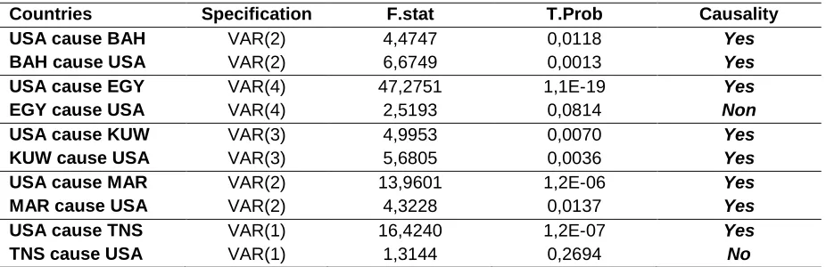
Table 16: Short-Term Causality Test (Crisis Period)

VAR(2) VAR(2) 4,4747 6,6749 0,0118 0,0013 Yes Yes

USA cause EGY EGY cause USA

VAR(4) VAR(4) 47,2751 2,5193 1,1E-19 0,0814 Yes Non

USA cause KUW KUW cause USA

VAR(3) VAR(3) 4,9953 5,6805 0,0070 0,0036 Yes Yes

USA cause MAR MAR cause USA

VAR(2) VAR(2) 13,9601 4,3228 1,2E-06 0,0137 Yes Yes

USA cause TNS TNS cause USA

VAR(1) VAR(1) 16,4240 1,3144 1,2E-07 0,2694 Yes No

Table 17: Long-Term Causality Test (Crisis Period)

VECM(2) VECM(2) 4,4747 6,6749 0,0118 0,0013 Yes Yes Note: As the table is provided directly to the probabilities associated test, we accept causation as the

(15)

Licensed under Creative Common Page 156 The emerged results following the causality test, three cases were detected "interdependence" (EGY-USA, MAR, TNS) and two cases of "pure contagion" (BAH and USA-KUW), which means the generation of new causal relationships after the outbreak of the "subprime" crisis.

This result shows evidence of the pure contagion hypothesis, which can led us to support the idea that the stock index is an aggregate indicator of the different shares issued in the domestic financial market and the decision of the investor to purchase or not depends much more on performance of the company as of the fundamental characteristics of the country.

It is wise to note that detected a single significant long-term causal relationship (USA-BAH), where it can lead to a long-term arbitration process, this result supports the idea that the Bahrain was affected by the crisis following the reputational externalities. Based on the citation from Summers (2000): "A crisis in one country can affect investors' expectations and perceptions about the structural conditions and vulnerabilities with respect to the other countries and the policy response must align many addition to these vulnerabilities." In other words and as already mentioned by Classens et al (2001), the pure contagion can be achieved if investors change their assessments of rules by which international finance is established.

SUMMERY AND CONCLUSIONS

The global financial crisis has been widely characterized as beginning with the real estate bubble burst and sub-prime crisis in the US. This was followed by a sharp decline in equity market indices in the US and subsequently in other countries. The crisis was not limited to advanced economies. Many emerging economies experienced even sharper decreases in stock indexes. Results issued by Dungey and Gajurel (2014) provide strong evidence of contagion effects from the US equity market to equity markets in both advanced and emerging markets. This paper examined the presence of "pure contagion" phenomenon during the "subprime" crisis between the United States and Bahrain. As well as US markets and those of Kuwait, we marked the presence of two cases of interdependence between the US markets and those of Egyptian partners and Moroccans. Thus, the direction of causality during the crisis period reveals an impressive dynamic between the US markets and those of the Gulf countries and shows a lesser degree with those of the other three countries of the treaty model.

(16)

Licensed under Creative Common Page 157 It should be noted that the causality study allows showing the existence of causality relationships and identifying their directions, but it does not specify the channels through which the crisis was transmitted from one country to another. It is also noteworthy that in our study we analyzed only one type of market, the stock market, of nine countries. It is much more relevant to consider a more diverse and wide sample of countries and focus on an analysis of several markets (sovereign debt market, stock market, money market, foreign exchange market) to explore the importance of interactions between these markets.

ACKNOWLEDGEMENT

Author thanks Slah Bahloul for detailed comments on an earlier version of the paper.

REFERENCES

Baig, T., Goldfajn, I., (1999), «Financial Market Contagion in the Asian Crisis», IMF Staff Papers 46, 167-195.

Bekaert, G., Ehrmann, M., Fratzscher, M., Mehl, A.J., (2011), «Global Crises and equity market contagion», NBER, Working Paper N° 17121.

Calvo, G., Mendoza E., (2000), «Rational Contagion and the Globalisation of Securities Markets», Journal of international economics, Vol.51, pp.79-113.

Corsetti, G., Pericoli, M., Sbarcia, M., (2005), «Some Contagion, some interdependence: more pitfalls in tests of financial contagion.», Journal of international Money and Finance, 24 (8), 1177-1199.

Dickey, D.A., Fuller W.A., (1981), «Likelihood Ratio Statistics for Autoregressive Time Series with a Unit Root», Econometrica, 49, 1057-1072.

Dickey, D.A., Pantula S., (1987), «Determining The Order of Differencing in Autoregressive Processes», Journal of Business and Economic Statistics, 15, 455-461.

Dungey, M., Fry, R., Gonzalez-Hermosillo, B., Martin, V., (2005), «Empirical modeling of contagion: a review of methodologies.», Quantitative Finance, 5 (1), 9-24.

Dungey, M., Martin, V., (2001), « Contagion across financial markets: an empirical assessment.», New Yok Stock Exchange Conference Paper, 16-17.

Dungey, M., Gajurel, D., (2014), «Equity market contagion during the global financial crisis: Evidence from the world’s eight largest economies.», Economic Systems, 38, 141-177.

Eichengreen, B., Rose A. K., Wyploz C., (1996), «Contagious Currency Crises», NBER,Working Paper N° 5681.

Engle, R.F., Granger C.W.J., (1987), «Cointegration and Error Correction: Representation, Estimating and testing», Econometrica, 55, 251-276.

Forbes, K., Rigobon, R., (1999), «Measuring Contagion: Conceptual and empirical issues», The Contagion Conference, World Bank.

Forbes, K., Rigobon, R., (2000), «Contagion in Latin America: Definitions, Measurement, and Policy Implications», NBER, Working Paper N°7885.

Forbes, K., Rigobon, R., (2002), «No Contagion, Only Interdependence, Measuring Stock Market Co-movement», Journal of Finance, 57(5), 2223-2261.

(17)

Licensed under Creative Common Page 158 Granger, C.W.J., (1969), «Investigating Causal Relations by Econometric Models and Cross-Spectral Methods», Econometrica, 36, 424-438.

Hamao, Y.R., R.W. Masulis and V.K. Ng., (1990),«Correlations in Price Changes and Volatility Across International Stock Markets», Review of Financial Studies, 3, 281-307.

Johansen, S., (1998), «Statistical Analysis of Cointegration Vectors», Journal of Economic dynamics and Control, 12, 231-254.

Kaminsky, G., Reinhart, C., (1998), «Leading Indicators of Currency Crises», IMF Staff Paper, 45, N° 1.

Kaminsky, G.L., Reinhart, C.M., (1998), «Financial Crisis in Asia and Latin America: Then and now», American Economic Review, 88(2), 444-448.

Kaminsky, Reinhart and Vegh,(2003), «The Unholy Trinity of Financial Contagion», NBER, Working Paper N°10061.

Kenourgios, D., Dimitriou, D., (2015), «Contagion of the Global Financial Crisis and the real economy: A regional analysis», Economic Modelling, 44, 283-293.

Masson,P., (1998), «Contagion: Monsnoonal Effects Spillovers, and Jumps Between Multiple Equilibria», IMF 142.

Masson, P., (1999,b), «Multiple Equilibria, Contagion and the Emerging Market Crises», IMF Working Paper N° 164.

Park, Y.C., Song, C.Y., (1999), «East Asian Crisis: One Year After», IDS Bulletin, 30, N°1, 93-103, Institute of Devlopment Studies, University of Sussex, Brighton, U.K.

Park, Y.C., Song, C.Y., (2001), «Institutional investors, trade linkage, macroeconomic similarities, and contagion of the Thai crisis.», Journal of Japanese International Economy, 15(2), 199-224.

Phillips, P.C.B., Perron, P., (1988), «Testing for Unit Root in a Time Series Regression»,Biometrika, 75, 335-346.

Rigobon, R., (1999), «On the Measurement of the International Propagation of Shocks», NBER, Working Paper N°7354.

Rose, A.K., Spiegel, M.M., (2009), «Cross-country causes and consequences of the 2008 crisis: early warning.»,NBER, Working Paper N°15357.

Rose, A.K., Spiegel, M.M., (2010), «Cross-country causes and consequences of the 2008 crisis: international linkages and Amercainexposure.»,Pacific Economic Revue,15 (3), 340-363.

Sander, H., Kleimeier, S., (2003), «Contagion and Causality: An Empirical Investigation of four Asian Crisis Episodes», International Financial Markets, 3, 171-186.

Van Rijckeghem, C., Weder, B., (2001), «Sources of contagion: is it finance or trade?», Journal of international Economics, 54 (2), 724-742.

(18)

APPENDICES

Figure 1: Evolution of stock index returns during quiet period (2005-2007)

Figure 2: Evolution of stock index returns during crisis period (2007-2009)

-.08 -.04 .00 .04 .08 .12

2005M07 2006M01 2006M07 2007M01

DLBA H -.12 -.08 -.04 .00 .04 .08

2005M07 2006M01 2006M07 2007M01

DLEGY -.08 -.04 .00 .04 .08 .12

2005M07 2006M01 2006M07 2007M01

DLKUW -.06 -.04 -.02 .00 .02 .04 .06

2005M07 2006M01 2006M07 2007M01

DLMA R -8 -4 0 4 8

2005M07 2006M01 2006M07 2007M01

DLOMA -.04 -.03 -.02 -.01 .00 .01 .02 .03 .04

2005M07 2006M01 2006M07 2007M01

DLTNS -.04 -.03 -.02 -.01 .00 .01 .02 .03

2005M07 2006M01 2006M07 2007M01

DLUSA -.24 -.20 -.16 -.12 -.08 -.04 .00 .04 .08