An Excel-Aided Method For Teaching
Calculus-Based Business Mathematics
Jiajuan Liang, University of New Haven, USA Linda Martin, University of New Haven, USA
ABSTRACT
Calculus-based business mathematics is a required quantitative course for undergraduate business students in most AACSB accredited schools or colleges of business. Many business students, however, have relatively weak mathematical background or even display math-phobia when presented with calculus problems. Because of the popularity of Excel, its ease of learning, and its rich computational functions, we have been teaching our calculus-based business mathematics in computer labs and accumulating feasible experience in employing Excel to assist our students’ learning in this course. In this paper we illustrate how to use Excel to enhance students’ understanding in difficult and important calculus-based mathematical principles and to find numerical solutions to difficult quantitative business problems by providing them with heuristic examples. Our experience shows that Excel can greatly simplify the interpretation of pure calculus principles and can substantially reduce students’ misunderstanding in applying calculus principles in solving quantitative business problems.
Keywords: Teaching, Excel, Calculus
1. INTRODUCTION
alculus-based business mathematics consists of two major topics: (1) derivative and its applications in business; and (2) integration and its applications in business. It is quite common that many undergraduate business students have weak prerequisite algebraic knowledge when entering this course. This creates a great challenge to both students and instructors when teaching this course by a traditional method without resorting to computer programs. For example, since many applications of calculus in business can be reduced to finding or summarizing quantitative information from various mathematical functions, an intuitive way of teaching calculus and its applications in business will be helpful for students to understand the key idea in calculus and the true meaning behind various mathematical principles. Function graphing or plotting is the easiest way to understand the theoretical properties of a mathematical function. Many computer programs provide powerful graphing or plotting options. Excel seems to be the easiest and widely available one with plotting options. Once the plot of a function is obtained, it becomes easily interpretable to summarize numerical information from the plot, and it is easily understandable to students in making numerical conclusions.
In order to provide the students with the opportunity to make use of the visual aspects of Excel, we conduct our classes in a computer lab classroom. After being presented with a problem, the students have the ability to immediately evaluate the functions and produce the graphs. This method incorporates aspects of experiential and problem based learning which have been found to enhance student knowledge (Hamer 2000 and Mykytyn 2007). The lab setting also necessitates that the student focus on the applications currently being presented because they will be expected to complete the assignment in class. When employing Excel to teach calculus-based business mathematics, it is essential to combine its graphing option with its powerful computational option. A complete version of Excel provides almost all commonly-used mathematical, financial, and statistical functions. It is sufficient to use these functions to solve many quantitative problems in undergraduate business courses (Arnold and Henry 2003 and Saibeni 2008). The purpose of this paper is to illustrate several important topics in calculus and its applications in business by examples. Section 2 will provide the details for illustration of derivatives and their applications in business. Section 3 gives the illustration of integration and its applications in business. Some concluding remarks are summarized in the last section.
12
2. EXCEL ILLUSTRATION FOR TEACHING DERIVATIVES
A. Break-Even Analysis
Break-even is a basic concept in business. It identifies the situation that a business activity will not result in a profit gain or profit loss, or simply zero profit. Identifying a production level or a sales level x with zero profit is equivalent to solving a mathematical equation like P(x)=0, where P(x) stands for the profit function associated with the production or sales level x. Therefore, mathematically, break-even analysis is equivalent to finding the zero point of a profit function. In some simple situations, there may be an easy analytical solution to an equation like P(x)=0.
In some complicated situations, no simple analytical solutions can be obtained but an approximate Excel solution can be easily obtained. See the following two examples.
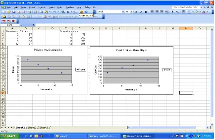
Example 1. A manufacturer of a popular automatic camera wholesales the camera to retail outlets throughout the United States. The past record shows the price-demand data as in Table 1 and the cost-quantity data in Table 2. (Data for all examples are from Barnett, et al. 2003)
Table 1 Price-Demand Data
Table 2 Cost-Quantity Data Demand x
(millions)
Price p ($) Quantity x
(millions)
Cost C(x)
(Million $)
2 87 1 175
5 68 5 260
8 53 8 305
12 37 12 395
A plot of the price-demand data and a plot of the cost-quantity data by using Excel are given in Figure 1. Plotting is accomplished by using the Chart Wizard command in Excel, chart type, XY Scatter. Both plots show a linear relationship between the two variables.
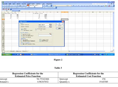
By using the regression option in Excel [Tools/Data Analysis/Regression], we can obtain the estimated linear relationship between price p and demand x, and the estimated linear relationship between the cost C(x) and demand x as given. (For an easier method to obtain the estimated linear relationships, we also use the “Add Trendline” function under the Chart command.) The Excel implementation of Regression is illustrated in Figure 2 and Excel output for is given in Table 3.
Figure 2
Table 3
Regression Coefficients for the Estimated Price Function
Regression Coefficients for the Estimated Cost Function
Intercept 94.75342466 Intercept 156
Demand x 4.96347032 Quantity x 19.65385
The demand and cost function are then as followed:
x
x
C
x
p
94
.
8
5
,
(
)
156
19
.
7
(1)The profit function P(x) is expressed as
P x
( )
R x
( )
C x
( )
, where R(x) represents revenue. Revenue is equivalent to price times quantity and is given by xp with the demand level x and the price p. So the profit function can be obtained from:156
1
.
75
5
)
7
.
19
156
(
)
5
8
.
94
(
)
(
)
(
x
xp
C
x
x
x
x
x
2
x
P
. (2)The break-even point x satisfies
0
156
1
.
75
5
)
(
x
x
2
x
P
. (3)14
15
1
x
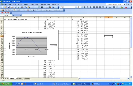
is given in Figure 3. To generate the plot, a column is created of incremental x values over its domain. Incremental x values are easily established by typing in the initial value of x in location A2, then placing the curser in location A3 and typing “=A2 + incremental value”. (In our example, we use 0.5 as the increment.) The copy function is then used to fill in the column. In a second column, type in “=-5*A2^2+75.1*A2-156” and use the copy function to fill in the remaining column. Once the values are established, Chart Wizard is employed to create the graph.
The plot of P(x) in Figure 3 shows that there are two break-even points in the two separate intervals [2, 3] and [12, 13]. By using the computational option in Excel, we can easily compute the values of P(x) for a set of discrete points in these two intervals and then search the approximate x-values such that
P
(
x
)
0
. We choose the values of x from 2 to 3 (using 0.01 as the increment) and from 12 to 13 (using 0.01 as the increment). We employ the same incremental Excel functionality as before. Then we can approximately identifyx
2
.
49
(
P
(
2
.
49
)
0
.
0015
) andx
12
.
53
(P
(
12
.
53
)
0
.
0015
) as the break-even points (see Figure 3). Theexact solution to equation (3) is
x
1
2.49002988
andx
2
12.5299701
1
. Therefore the approximate solution by Excel is quite close to the exact solution by analytical method. It is obvious that when choosing a smaller increment (say 0.001), Excel gives a fairly accurate solution to equation (3) as long as the increments are kept small.This method for searching for the zero point of a function is useful for much more complicated problems in quantitative business applications. The following example illustrates a more technical application.
Figure 3 (Continued)
Example 2. A mail-order company specializing in computer equipment has collected the data in Table 4, showing the weekly demand x for Data-Link modems at various prices p. The company purchases the modems from the manufacturer for $100 each. A simple plot of the demand equation indicates that the relationship is non-linear.
Therefore, we try to use an exponential function (
p
ab
x) to find the break-even price (to the nearest cent). After a review of basic logarithm rules, an Excel solution can be demonstrated to the students.Table 4
Demand x Price per modem p ($)
412 169.95
488 149.95
575 139.95
722 129.95
786 119.95
In order to use the regression option in Excel, we need to linearize the exponential regression
p
ab
x by taking the logarithm:)
ln(
)
ln(
)
ln(
p
a
x
b
(4)By applying the regression option to the data in Table 4 for equation (4), we can obtain the estimated regression equation
ln(
p
)
5
.
4469
0
.
0008
x
. This gives the estimated price function)
0008
.
0
4469
.
5
exp(
x
16
x
x
x
x
P
(
)
exp(
5
.
4469
0
.
0008
)
100
(5)(Alternatively, using the “Add Trendline” function on the Chart command and selecting the exponential form type, yields the following function:
x
e
p
232
.
03
0.008and the profit function becomes
x
e
x
x
P
(
)
(
232
.
03
0.008x)
100
.This method only requires a review of the concept of “e” and limits the use of logarithms. The functional values remain the same.)
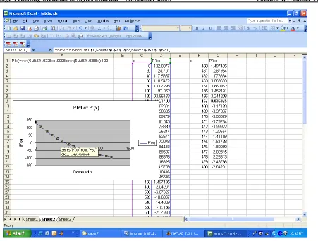
The plot of P(x) by Excel in the range
0
x
1200
is given in Figure 4. It shows that the meaningful break-even point occurs in the interval [1020, 1040]. An Excel computation from x=1020 (1) to 1040 (choosing 1 as the increment) for the profit function shows that the break-even point is located in [1052, 1053]. Since x denotes the number of modems, the approximate solution to the break-even point is x=1052. The exact solution to P(x)=0 from equation (5) is x=1052.1623. Therefore the approximate solution by Excel is still quite close to the exact solution by analytical method.B. Increasing And Decreasing Intervals
In business applications, it is important for a production manager or sales manager to know when the production or sales activity will lead to gain or loss. This is equivalent to identifying when the profit function is increasing and when it is decreasing. The calculus principle for increasing (or decreasing) is associated with positive (or negative) derivative of the profit function. Identifying the increasing (or decreasing) interval of a function is equivalent to solving a mathematical inequality associated with the derivative function. While this is not a challenge for students with good algebraic background, it may be difficult to those students without sufficient algebraic knowledge. Furthermore, an inequality may not have a simple analytical solution. Therefore, manual calculation in traditional teaching without resorting to computer programs could be no longer applicable. The following two examples illustrate a simple and a relatively complicated case, respectively.
Example 3. (Example 1 continued) Figure 3 in Example 1 shows that the profit function is increasing before it reaches the maximum and it is decreasing after the maximum. In order to identify the increasing and decreasing interval, we need to obtain the derivative function. Prior to approaching this example, students are presented with the elementary rules of differentiation and the methods of obtaining optimal points. So that the derivative of the profit function can be derived:
1
.
75
10
)'
156
1
.
75
5
(
)
(
'
x
x
2
x
x
P
and then solved for the optimal point x from
P x
'( )
0
, which gives51
.
7
0
1
.
75
10
x
x
. (6)By plotting the derivative function it is easy to see when
x
7
.
51
,
P
'
(
x
)
0
and so P(x) is increasing forx<7.51. When
x
7
.
51
,
P
'
(
x
)
0
and so P(x) is decreasing for x>7.51. This implies that there is a gain when the demand level x<7.51 (millions) and there is a loss when x>7.51 millions.Example 4. (Example 2 continued) Figure 4 in Example 2 shows that the profit function is increasing before it reaches the maximum and it is decreasing after the maximum. In order to identify the increasing and decreasing interval, we need to obtain the derivative function:
.
100
)
0008
.
0
4469
.
5
exp(
0008
.
0
)
0008
.
0
4469
.
5
exp(
]'
100
)
0008
.
0
4469
.
5
exp(
[
)
(
'
x
x
x
x
x
x
x
P
(7)It is obvious that there is no simple analytical solution to the inequality
P
'
(
x
)
0
orP
'
(
x
)
0
forP
'
(
x
)
given18
Figure 5
Figure 5 shows that the point x such that
P
'
(
x
)
0
occurs in the interval [460, 480]. Using an incrementof 1, we can approximate when
P
'
(
x
)
0
. Excel computation in Figure 5 shows that when x=467,0364
.
0
)
(
'
x
P
, which is the closest point such thatP
'
(
x
)
0
. From Figure 5, we can approximately identify0
)
(
'
x
P
for x<467 andP
'
(
x
)
0
for x>467. Therefore, the increasing interval is x<467 and the decreasing interval is x>467. This implies that there is a gain when the demand level x<467 and there is a loss when the demand level x>467.C. Optimization
Optimization is the most important topic in teaching calculus-based business mathematics. Optimization of
a function f(x) in a domain D is to identify the value, say
x
x
0, of a variable x such thatf
(
x
0)
is either the maximum value or the minimum value of the function within the domain, that is,either
f
(
x
0)
max
f
(
x
)
D x
orf
(
x
0)
min
f
(
x
)
D x
. (8)Example 5. (Example 1 continued) We want to find a suitable demand x (millions) for cameras and price in Table 1 so that the maximum profit can be obtained. A plot of the profit function P(x) is given in Figure 3. It shows that the maximum profit exists. The suitable demand x for maximum profit satisfies (see equation (6)):
0
1
.
75
10
)'
156
1
.
75
5
(
)
(
'
x
x
2
x
x
P
(9)It turns out that x=7.51 (millions) and the suitable price is obtained from the estimated price function in equation (1):
p
94
.
8
5
7
.
51
$
57.25
per camera.
Finding the zero point analytically for a simple function can be as simple as in the above Example 5. When the analytical solution cannot be readily obtained, Excel can help to obtain the almost accurate solution. See the following example.
Example 6. (Examples 2 and 4 continued) We want to find a suitable demand x (number of modems) and price from the data in Table 3 so that the maximum profit can be obtained.
A plot of the profit function P(x) is given in Figure 4. It shows that the maximum profit exists. The suitable demand x for maximum profit satisfies (see equation (7)):
.
0
100
)
0008
.
0
4469
.
5
exp(
0008
.
0
)
0008
.
0
4469
.
5
exp(
)
(
'
P
x
x
x
x
(10)It is obvious that there is no simple analytical solution to this equation. The Excel calculation in Figure 5 shows that
0
0364
.
0
)
467
(
'
P
. So the best integer solution to equation (10) is x=467 modems to obtain the maximum profit. The corresponding best price is obtained from the estimated price function70
.
159
$
)
467
0008
.
0
4469
.
5
exp(
p
per modem from equation (5).3. EXCEL ILLUSTRATION FOR TEACHING INTEGRATION
Integration consists of definite and indefinite integrals. It is the most challenging topic in teaching calculus-based business mathematics. Since indefinite integrals are mostly pure mathematical problems, we focus on definite integrals. Integration problems can only be solved for simple functions or by using existing formulas. For situations of complicated functions or no existing formulas, the Simpson formula can be employed to obtain an approximate solution. The approximation can be made as good as possible for functions with bounded second derivatives (this is true for many business functions) by using Excel. Let
b
x
x
x
x
x
a
0
1
2
n1
n
(11)be a partition of a given interval [a, b], where n is the number of partition points which are equally-spaced with a distance
x
(
b
a
)
/
n
. Definex
x
x
f
M
dx
x
f
I
n k k k n ba
1 12
sum
M idpoint
,
)
(
. (12)Simpson’s formula for computing the integral I in (12) is to compute the midpoint sum
M
n and useM
n to approximate I. The accuracy of this approximation is guaranteed by the error bound (see, e.g., Barnett, Ziegler, and Byleen, 2003, page 407):2 3 2
24
)
(
|
|
n
a
b
B
M
I
n
, where 2max |
''( ) |
a x b
B
f
x
20
It can be seen from (13) that the accuracy of approximating the integral I by
M
n in (12) can be made as good as possible by choosing the number of equally spaced partition points n as large as possible.
Use of the Simpson formula is an excellent way to demonstrate that bounded integration is equivalent to area. The Simpson formula constructs small rectangles whose individual area is given by its length times its width.
The length of the rectangle is
)
2
(
x
k 1x
kf
and the width is measured by
x
(
b
a
)
/
n
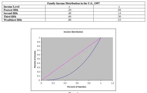
.Example 7. The distribution of income among families in individual countries is an important measurement in welfare economics. Income distribution is represented by computing the per cent share of total income held by each successive fifth of the population. For example, income distribution for the U.S. in 1997 is given in Table 5. The table shows that the lowest fifth of the population received 4% of the total income of the U.S. The graph of y = f(x)
is obtained through regression and is called the Lorenz curve. An example of a Lorenz curve for
y
x
2.6 in given in Figure 6.Table 5
Family Income Distribution in the U.S., 1997
Income Level x y
Poorest fifth .20 .04
Second fifth .40 .14
Third fifth .60 .30
Wealthiest fifth .80 .53
Incom e Distribution
0 0.1 0.2 0.3 0.4 0.5 0.6 0.7 0.8 0.9 1
0 0.2 0.4 0.6 0.8 1 1.2
Percent of Fam ilies
P
e
rc
e
n
t
o
f
In
c
o
m
e
Figure 6
The index of income concentration is the ratio of the area bounded by y = x and the Lorenz curve to the area of the triangle under the line y = x (which is equal to ½).
1
0
index
2 ,
I
I
[
x
f x dx
( )]
. (14)The area between y = x and the Lorenz curve can be found using Simpson’s formula. The Simpson formula for approximating the integral I in (14) is to compute the midpoint sum
M
n given by (12). Since theaccuracy requirement is three decimal places, we choose
10
3
0
.
001
as the equal distance between any two partition points. That is,
x
(
b
a
)
/
n
0
.
001
with a=0 and b=1. Therefore, the number of partition points1000
001
.
0
/
)
0
1
(
n
. The steps for the numerical computation of the integral I in (14) are as follows.Step 1. Create a column of x-data beginning with x=0 and ending with x=1 by using the increment 0.001. For example, in column C in Figure 7, type “0” in cell C2 (C-column, row #2) and then type “=C2+0.001” in cell C3 and enter it. Use the copy function to extend the calculation to the whole C column until the number 1 is reached;
Step 2. Create a column of “x-midpoint”. For example, in column D in Figure 7 beginning with cell D3, type “=(C2+C3)/2” and enter it. Use the copy function to extend the calculation to the whole D column until reaching the number 1;
Step 3. Create a column of “y at midpoint”, which means that the y-function is evaluated at the x-midpoint value. For example, in column E in Figure 7 beginning with cell E3, type “=D3- D3*2.6)” and enter it. Use the copy function to extend the calculation to the whole D column until reaching the number 1.
Step 4. Compute the Simpson sum, which is the midpoint sum
M
n defined in (12). On column F3, enter=F3*0.001 (since Δx =0.001). Use the Σ function to add column F. The final result
I
0
.
222
is the value of the integral (14). See Figure 6 (continued). The index of income concentration can then be computed as 2 ×.222 = .444.22
Figure 7 (Continued)
The error bound from using the Simpson sum (midpoint sum)
M
n
0
.
222
as the approximate value of integral I in (14) can be obtained by using (13). It can be computed that
2
2.6 .6
2
''( )
d
4.16
f
x
x
x
x
dx
(15)It can be obtained that .6
0 1 0 1
max |
''( ) | max | 4.16
| 4.16
x
f
x
xx
. Therefore, by using the Simpson error bound(13), the error bound by using
M
n
0
.
222
to approximate the integral (14) is3 3
7 2
2 2
(
)
4.16(1 0)
|
|
1.73 10
24
24(1000)
n
B b a
I
M
n
. (16)The approximation is almost perfect. This shows that integration problems can be well approximated by using Simpson formula and Excel. The error can be made as small as possible by choosing the equally-spaced partition points as large as possible.
4. CONCLUDING REMARKS
appropriate learning vehicle for our students. Third, students entering into more advanced quantitative analysis courses are more fluent in Excel techniques and thereby adapt more quickly to new assignments. The use of a computer lab or personal laptops in the classroom is changing the way many courses are taught and our examples show how these technologies can be combined with common business software (Excel) to enhance student learning (Bell 2008). We have found that students appreciate using Excel and feel that that have learned more in the course.
AUTHOR INFORMATION
Jiajuan Liang is an Associate Professor of Management at the University of New Haven. He has a Ph.D. in Multivariate Statistics from the Hong Kong Baptist University. He has published his research in statistics in journals such as Psychometrika and the Journal of Statistical Planning and Inference.
Linda Martin is a Professor of Management at the University of New Haven. She holds a Ph.D. in economics from the University of South Carolina. Her recent area of research has been on improving education and she has published in the Journal of Education for Business. Prior publications have been in the Monthly Labor Review and the Quarterly Journal of Business and Economics.
REFERENCES
1. Arnold, T., Henry, S. (2003). Visualizing the stochastic calculus of option pricing with Excel and VBA.
Journal of Applied Finance 13(1), 56-66.
2. Barnett, R., Ziegler, M., and Byleen, K. (2003). Applied Calculus, 8th edition. Pearson Prentice Hall, Upper Saddle River, New Jersey.
3. Bell Jr, R. and Glen, A. (2008). Experiences Teaching Probability and Statistics with Personal Laptops in the Classroom Daily. The American Statistician 62(2), 155.
4. Hamer, L. (2000). The Additive effects of Semistructured Classroom Activities on Student Learning: An Application-Based Experiential Learning Techniques. Journal of Marketing Education 22(1), 25-34. 5. Mykytyn, P. (2007). Educating Our Students in computer Application concepts: A Case for Problem-Based
Learning. Journal of Organizational and End User Computing 17(1), 51-62.