CSUSB ScholarWorks
CSUSB ScholarWorks
Electronic Theses, Projects, and Dissertations Office of Graduate Studies
6-2015
Elliptic Curves
Elliptic Curves
Trinity Mecklenburg
Follow this and additional works at: https://scholarworks.lib.csusb.edu/etd Part of the Algebra Commons
Recommended Citation Recommended Citation
Mecklenburg, Trinity, "Elliptic Curves" (2015). Electronic Theses, Projects, and Dissertations. 186. https://scholarworks.lib.csusb.edu/etd/186
A Thesis
Presented to the
Faculty of
California State University,
San Bernardino
In Partial Fulfillment
of the Requirements for the Degree
Master of Arts
in
Mathematics
by
Trinity Leaire Mecklenburg
A Thesis
Presented to the
Faculty of
California State University,
San Bernardino
by
Trinity Leaire Mecklenburg
June 2015
Approved by:
Ilseop Han, Committee Chair Date
Zahid Hasan, Committee Member
John Sarli, Committee Member
Charles Stanton, Chair, Corey Dunn
Abstract
The main focus of this paper is the study of elliptic curves, non-singular
pro-jective curves of genus 1. Under a geometric operation, the rational points E(Q) of an
elliptic curve E form a group, which is a finitely-generated abelian group by Mordell’s
theorem. Thus, this group can be expressed as the finite direct sum of copies of Z and
finite cyclic groups. The number of finite copies of Zis called the rank of E(Q).
From John Tate and Joseph Silverman [ST92], we have a formula to compute
the rank of curves of the form E :y2 =x3+ax2+bx. In this thesis, we generalize this
formula, using a purely group theoretic approach, and utilize this generalization to find
the rank of curves of the form E :y2 =x3+c. To do this, we review a few well-known
homomorphisms on the curve E :y2 =x3+ax2+bxas in Tate and Silverman’s Elliptic
Curves [ST92], and study analogous homomorphisms on E : y2 = x3 +c and relevant
Acknowledgements
I would like to thank all of the wonderful professors I have had at CSUSB. I am
grateful for all they have taught me. I would like to thank Professor Chavez for always
having an enjoyable class and making so much sense. I know he deserves to retire someday,
but part of me hopes he never does. I would also like to thank Professor Trapp for having
an enjoyable class, his personality and his one-of-a-kind laugh. He patiently gave me
countless office hours and stayed after every test to go over the problems that would have
caused me insomnia if they were left unanswered. I would like to thank Professor Ventura
for convincing me that I was competent enough to do the MA program. I would also like
to thank Professor McMurran for going above and beyond her job duties. I could not
possibly list all of the things I would like to thank her for. She is a mentor to me and has
a vested interest in her students, like no other. Thank you to my committee members,
Professor Hasan and Professor Sarli. I appreciate all the time they have given me. A
special thanks to Professor Han for introducing me to this topic and for his excitement
for it. He is an excellent teacher. I have learned so much from him, not just about elliptic
curves, but about how to write mathematics and about life. He has given me so much of
his time, unpaid. If I ever happen upon a large sum of money, I will definitely send it his
way.
I would like to thank John Tate and Joseph Siverman for writing a book that
really simplified elliptic curves. Their ability to bring an advanced topic down to an
undergraduate level really shows their mastery of the topic. Without their book, I really
wouldn’t have had an entry point to this topic.
I would like to thank all of the exceptional people I met throughout the
pro-gram, my study budies Jeff, Joe, Leonard, Matt and Stephanie. Our talks usually led to
solutions, and if they didn’t it was comforting to have someone to be lost with. I would
really like to thank Joe for pushing me to be better. I have so much admiration for him.
I would also like to thank Stephanie for teaching me so much. I went into this program
hoping to get a master’s degree, but I came out with something better, her friendship.
Finally, I would like to thank my husband. He never once harrassed me for
taking way too long to complete this program. He believed in me even when I didn’t
Table of Contents
Abstract iii
Acknowledgements iv
List of Figures vi
1 Quadratic Polynomials 1
1.1 Review of the Projective Plane . . . 1
1.2 Rational Points on Quadratic Polynomials . . . 5
1.3 Rational Points on Cubic Polynomials . . . 16
1.4 Formulas for the Group Law . . . 26
1.5 Properties of Points of Finite Order . . . 28
2 Curves of the Form y2=x3+ax2+bx+c 34 2.1 Mordell’s Theorem . . . 34
2.2 Some Useful Homomorphisms . . . 35
2.3 Modules and Exact Sequences . . . 43
2.4 The Rank ofE(Q) . . . 49
3 Curves of the Form y2=x3+c 58 3.1 Homomorphisms for the New Curve . . . 58
3.2 A New Formula for Rank . . . 72
4 Conclusion 78
List of Figures
1.1 Two Distinct Lines Intersecting at Two Points . . . 4
1.2 Theorem 1.2.1 . . . 6
1.3 Rational Points on the Unit Circle . . . 7
1.4 The Composition of Two Distinct Points on a Cubic . . . 17
1.5 The Composition of Two Non-Distinct Points on a Cubic . . . 17
1.6 Identity For a Single Point Under∗ . . . 18
1.7 The Group Operation⊕ . . . 19
1.8 Verification ofOas the Identity Element . . . 21
1.9 The Inverse ofP . . . 22
1.10 Investigating Associativity . . . 22
1.11 A Singularity For Whichf(x) Has a Double Root, Forming a Node . . . . 24
1.12 A Singularity For Whichf(x) Has a Triple Root, Forming a Cusp . . . . 24
1.13 ProjectingP Ontox= 1 . . . 25
1.14 f(x) with Three Real Roots . . . 30
1.15 f(x) with One Real Root . . . 30
1.16 Finding 2P . . . 32
Chapter 1
Quadratic Polynomials
1.1
Review of the Projective Plane
A major focus of this paper is the group of rational points on an elliptic curve.
These elliptic curves will be embedded in the projective plane. Hence a brief review of the
projective plane will be given. We will give two different descriptions of the projective
plane, one algebraic and one geometric, since it will be useful in certain situations to
think of one way over the other.
Algebraic Definition of the Projective Plane
Consider the Fermat equation
xN+yN = 1, (1.1)
with rational solutions. Let x= ac and y = db be solutions such that the fractions are in
lowest terms and the denominators are positive. If we substitute the solutions into (1.1)
and clear the denominators, we have
aNdN+bNcN =cNdN.
Now it is clear that cN |aNdN. Since ac is in lowest terms,a and c are relatively prime.
Thus cN |dN, implying c |d. By a similar argument, we can conclude that d|c. Thus
There-fore, c=d.
Any rational solution to (1.1) has the form ac,bc
and will have (a, b, c) as a
corresponding integer solution to
XN +YN =ZN. (1.2)
Notice that as long as c 6= 0, the converse is true as well. That is, any integer solution
(a, b, c) to (1.2) will also have the corresponding rational solution ac,bc to (1.1). In fact, any triple (λa, λb, λc) for λ6= 0 will satisfy (1.2) and will correspond to ac,bc as a solu-tion for (1.1).
Let’s proceed to lay the foundation of the projective plane and see how it earned
its name. Imagine that the origin inR3is an eye, and that there is a screen (or a plane) in
R3. Each point on the plane is in one-to-one correspondence with a line passing through
the point and the eye. We will use this line to describe projective points.
Definition 1.1.1. Aprojective point is a line inR3 that passes through the origin ofR3.
Notice that we only need one point inR3 besides the origin to describe a line in
R3, and this point is not unique. For example, the line in R3 passing through the origin
and (1,2,3) is the same line that passes through the origin and (2,4,6). This leads us to
the following definition.
Definition 1.1.2. The projective plane is the set of triples [a, b, c], with a, b and c not
all zero, such that two triples [a, b, c] and [a0, b0, c0] are considered to be the same point if
there is a non-zero λsuch thata=λa0,b=λb0 andc=λc0. The numbersa,band care
called homogeneous coordinates for the point [a, b, c].
We will denote the projective planeP2. Brackets will always describe a
An algebraic curve in the affine planeA2 is defined to be the set of solutions to
a polynomial equation in two variables, f(x, y) = 0. Fermat equation (1.1) is an example
of such a curve. Curves in P2 will be given by polynomials in three variables,F(X, Y, Z)
such that if F(a, b, c) = 0, then F(λa, λb, λc) = 0 for all λ.
Definition 1.1.3. A polynomial F(X, Y, Z) is a homogeneous polynomial of degree d if
it satisfies the identity
F(λX, λY, λZ) =λdF(X, Y, Z).
A projective curve C inP2 is the set of solutions to a non-constant homogeneous
polyno-mial.
Now, if we look back at the homogeneous polynomial given by Fermat equation
(1.2), we can see that there are some problematic homogeneous coordinates we need to
deal with. For example, [0,0,0] is a solution to (1.2), but it has no corresponding rational
point ac,bc
. We will consider [0,0,0] as trivial and will discard it. Notice, [0,0,0] is not
defined in Definition 1.1.2. We need a point distinct from [0,0,0] to define a projective
point. Also, if N is odd, then [1,−1,0] and [−1,1,0] are nontrivial solutions to (1.2)
that do not correspond to any rational solutions to (1.1), at least not when using the
conventional method.
Consider the sequence of solutions [ai, bi, ci] to (1.2) where [ai, bi, ci]→[1,−1,0]
asi→ ∞andai,biandciare allowed to be real numbers. The corresponding solutions to
(1.1) approach (∞,∞). Thus we will have to extend the affine planeA2to include “points
at infinity,” so that the homogeneous coordinates [1,−1,0] and [−1,1,0] correspond to
these points. This brings us to our second definition of the projective plane.
Geometric Derivation of the Projective Plane
Before we begin developing the projective plane geometrically, we must define
what a line is inP2.
Since a projective line is really a plane inR3, a line can be thought of as the set
of points [a, b, c]∈P2 whose coordinates satisfy an equation of the form
αX+βY +γZ= 0
for some constants α,β and γ not all zero.
Any beginning course in Euclidean geometry will include the following
postu-lates:
(i) Two distinct points determine a unique line.
(ii) If two distinct lines intersect, then they intersect in exactly one point.
In the projective plane, we are going to add points at infinity so that parallel
lines intersect. Then there will be no distinction between parallel and non-parallel lines.
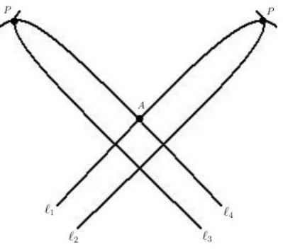
Now the question remains as to how many points at infinity we should add. What if we
add one point at infinity, say P? Consider two sets of parallel lines such that`1 k`2 and
`3 k`4, as depicted in Figure 1.1. Then `1 and `2 intersect atP, and`3 and `4 intersect
at P as well. Hence, all four lines intersect at P. This creates a problem since we are
trying to construct the projective plane so that postulates (i) and (ii) still hold. Property
(ii) does not hold since, for example,`1 and `4 intersect atA and P.
For this reason, we add points at infinity for each direction (slope), so that each
line in P2 consists of a line in A2 together with a point at infinity corresponding to the
line’s direction. Two lines have the same direction if and only if they are parallel. This
leads us to our geometric definition of the projective plane.
Definition 1.1.5. Theprojective plane
P2 =A2∪ {the set of directions inA2},
where the extra points inP2 associated to directions, that is the points inP2 that are not
in A2, are calledpoints at infinity, and the set of points at infinity is considered to be a
line L∞whose intersection with any other line Lis the point at infinity corresponding to
the direction ofL.
1.2
Rational Points on Quadratic Polynomials
Now that we have defined the projective plane, we are ready to look at some
Diophantine equations and lay the foundations for the group we are going to investigate.
In order to better study our group and its operation, let’s start by considering the
ratio-nal points that satisfy simpler polynomials that we are familiar with. We will start with
quadratic polynomials, or conics, since much is known about their behavior.
Recall that a line of the form ax+by+c = 0 is a rational line if a, b and c
are all rational, and a point (x, y) is a rational point if both its coordinates are rational
numbers. If a line is drawn through two rational points, then the line will be a rational
line. We can see this is true by using the point-slope formula to derive the equation of the
line that passes through the given points. Since Q is field, all of the operations used to
simplify the point-slope equation will result in rational coefficients. Also, if two rational
lines intersect, their intersection is a rational point. All of the operations used to solve
the system would again be closed since Qis a field.
rational? Upon solving the system, the resulting x-coordinates would be solutions to a
quadratic equation with rational coefficients. So the points of intersection of the rational
line with the rational conic will be rational if the solutions to the quadratic equation are
rational. It is important to note for future reference that if one point of intersection is
rational, then the other is as well. If one of the points of intersection is irrational, then
the other is as well since it is its conjugate.
We might question next if we could find all of the rational points on a rational
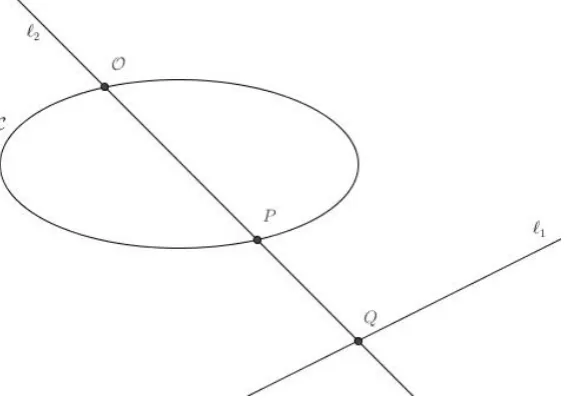
conic. To start, assume we know one rational pointOon the given conic. We can draw a
rational line `1 and project the conic onto `1 from O. Every line connecting Oto`1 will
intersect the conic at another point. We will consider the line tangent atOas intersecting
the conic at O twice. This gives a one-to-one correspondence between any point on the
conic and its corresponding point on`1.
Figure 1.2: Theorem 1.2.1
Theorem 1.2.1. Let C be a rational conic, O be a rational point and `1 be a rational
line. Let `2 be a line that connectsO with `1 and that intersects the conic again at point
P. Let the intersection of `1 and `2 be the point Q. The point P is a rational point if
Proof. IfP is rational, then there are two rational points on`2, making it a rational line.
We are given that `1 is a rational line. We showed earlier that the intersection of two
rational lines is a rational point. Therefore, Qis a rational point.
Conversely, ifQ is rational, then there are two rational points on`2, so again it
is a rational line. We saw earlier that the intersection of a rational line with a conic could
produce rational or irrational solutions to a quadratic, but if we knew that one solution
was rational, the other was as well. Since we know that O is rational, we have thatP is
rational.
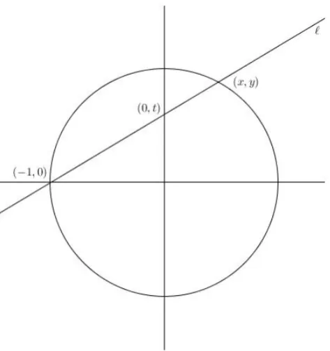
Example 1.2.1. Find all of the rational points on x2+y2= 1.
Solution. Using the logic from above, let’s find the proper choice for our rational point
and rational line. A good choice for the rational line is the y-axis. Let’s use (−1,0)
as the rational point on the circle. Then the equation of any line ` through (−1,0) is
y =t(1 +x), wheret is they-intercept.
To find all of the rational points (x, y) on the circle, we need to find the
inter-section of `and the circle. From the circle, we havey2 = 1−x2. From the line, we have
y2 =t2(1 +x)2. So 1−x2 = t2(1 +x)2. We already know (−1,0) is both on the circle
and line, so x=−1 is obvioulsy a root of this equation. Forx6=−1,
1−x2 = t2(1 +x)2
(1 +x)(1−x) = t2(1 +x)2
1−x = t2(1 +x).
Solving for x in terms oft, we have
1−t2 = t2x+x
x = 1−t
2
1 +t2.
Substituting this result into y=t(1 +x) gives us
y = t
1 +1−t
2
1 +t2
y = 2t 1 +t2.
Thus, for anyt∈Q, the map t→1−t2
1+t2,1+2tt2
will allow us to find all rational
points on the unit circle except for (−1,0), which we get if we lett→ ∞. On the other
hand, fromy=t(1 +x), we have that the map (x, y)→ 1+yx will map any rational point
(x, y) on the unit circle, aside from (−1,0), to the set of rational points Q. The point
(−1,0) would of course map to the point at infinity. To sum up, there is a one-to-one
correspondence between the set of rational points on the unit circlex2+y2= 1 and the
set Qof rational points by given by the maps above.
The formulas derived above also play an integral role in finding formulas to
de-scribe the lengths of the sides of all primitive right triangles.
Definition 1.2.1. A Pythagorean triple is a set of positive integers, a, b and c, written
If (a, b, c) is a Pythagorean triple, then so is (ka, kb, kc) for any positive integer k.
Definition 1.2.2. We say that a Pythagorean triple isprimitiveifa,bandcare coprime,
that is, gcd(a, b, c) = 1.
The following two lemmas will be useful in the derivation of formulas that
de-scribe all primitive Pythagorean triples.
Lemma 1.2.2. If (a, b, c) is a primitive Pythagorean triple, then a and b have opposite
parity.
Proof. Since (a, b, c) is a primitive Pythagorean triple,a2+b2=c2and gcd(a, b, c) = 1. If
aandbwere both even, then their squares would be even. The sum of two even numbers
is again even. Then c2 is even, from which it follows that c is even. Thus, 2 dividesa,b
and c. This contradicts the fact that gcd(a, b, c) = 1.
Ifaand b were both odd, then their squares would be odd. Perfect squares are
congruent to either 0 or 1 modulo 4 depending on if they are even or odd, respectively.
Thena2 ≡b2 ≡1 (mod 4), implying thata2+b2≡2 (mod 4). On the other hand,c2 ≡0
or 1 (mod 4). This contradicts the fact that a2+b2 =c2. Hence, aand bcannot both be
odd either. Therefore, aand b have opposite parity.
Lemma 1.2.3. A Pythagorean triple (a, b, c) is primitive if and only if any two of a, b
and c are relatively prime.
Proof. Let (a, b, c) be a primitive Pythagorean triple, that is,a2+b2=c2and gcd(a, b, c) =
1. If any two of a,b and cwere to have a common factor, then that factor would divide
the sum or difference of their squares, and consequently, the remaining number of a, b
and c. This contradicts the given that gcd(a, b, c) = 1. Thus, any two of a, b and c are
Conversely, assume that for the Pythagorean triple (a, b, c) any two ofa,b and
c are relatively prime. If any two of a, band cdo not share a common factor, then it is
clear that all three do not have a common factor. Thus, the Pythagorean triple (a, b, c)
is primitive.
Example 1.2.2. Derive formulas to describe all primitive Pythagorean triples.
Solution. Let’s find integersX,Y, andZsuch thatX2+Y2 =Z2. Assume gcd(X, Y, Z) =
1 so that we have a primitive right triangle. By Lemma 1.2.2, X and Y have opposite
parity. Suppose X is odd and Y is even and dehomogenize X2 +Y2 = Z2, so that
x2+y2 = 1 where x= XZ and y = YZ. Then (x, y) is a rational point on the unit circle.
From Example 1.1, we know that
x= 1−t
2
1 +t2 and y=
2t
1 +t2.
Letting t= mn form and nrelatively prime, the formulas above simplify to
X
Z =x=
n2−m2 n2+m2 and
Y
Z =y=
2mn n2+m2.
By Lemma 1.2.3,X andZ are relatively prime, as well asY and Z. Thus, there
exists a positive integerksuch thatkX =n2−m2,kY = 2nm, andkZ =n2+m2. Let’s
show that k = 1. Since kX =n2−m2 and kZ =n2+m2, it follows that k| n2−m2
and k | n2+m2. Thus k divides any linear combination of n2 −m2 and n2 +m2, in
particular, k|2n2 and k |2m2. So k|gcd(2n2,2m2) = 2gcd(n2, m2). Since we assumed
gcd(n, m) = 1, it follows that gcd(n2, m2) = 1. Thus k|2. So either k = 1 ork= 2. If
k = 2, then n2−m2 is even, implying that n and m have the same parity. Ifn and m
are both odd or both even, then n2−m2 ≡0 (mod 4) using the logic from the proof of
Lemma 1.2.2. However, since X is odd, 2X ≡2 (mod 4), which reaches a contradiction.
Hence, we have k = 1. Therefore, in order to find the side lengths X, Y and Z of any
primitive right triangle, you can substitute any relatively prime integersm and ninto
The findings above lead us to the theorem that follows. We used a geometric
approach to develop the formulas above. Now we will take an algebraic approach to prove
the theorem below.
Theorem 1.2.4. If (a, b, c) is a primitive Pythagorean triple (withb even), then
a=n2−m2, b= 2nm, and c=n2+m2
wherenandmare positive integers withn > m, gcd(n, m) = 1andnandmhave opposite
parity. Conversely, for n andm as above, (a, b, c) yields a primitive Pythagorean triple.
Proof. Let (a, b, c) be a primitive Pythagorean triple withb even. Then a2+b2 =c2, or
equivalently, b2=c2−a2. Since bis even, b2 is even. From which it follows thatc2−a2
is even. From Lemma 1.2, we know thataand bhave opposite parity, so amust be odd.
If a is odd, then a2 is odd. Hence, c2 must be odd as well in order for c2 −a2 to even.
So we have that bothaandcare odd. Then we can conclude thatc+aandc−aare even.
Let gcd(c+a, c−a) = d. Then d | c+a and d | c−a. Thus, d divides any
linear combination of c+a and c−a, in particular, d | 2a and d | 2c. It follows that
d | gcd(2a,2c) = 2 gcd(a, c). Given that (a, b, c) is a primitive Pythagorean triple, by
Lemma 1.2.3, a and c are relatively prime. Hence, d|2. So gcd(c+a, c−a) is either 1
or 2. We showed above that c+aand c−a are both even, so it must be the case that
gcd(c+a, c−a) = 2. Thus, gcd(c+2a,c−2a) = 1.
Since b42 = c+2a c−a
2
and c+2a and c−2a are relatively prime, c+2a and c−2a must
be perfect squares. Let c+2a =n2 and c−2a =m2. Thenn2−m2 = c+2a− c−a
2 =a. Also,
2mn= 2
q
c−a
2
q
c+a
2 = 2
q
c2−a2
4 =
√
c2−a2=√b2 =b. Finally, n2+m2= c+a
2 +
c−a
2 =
c.
Now if m, n > 0, then n > m since a= n2−m2, and a side of a triangle can
factor, any two of a,b and c would not be relatively prime, contradicting Lemma 1.2.2.
From Lemma 1.2.3, sincebis even, aand care odd. Sincen2−m2 =aandn2+m2=c,
it follows that nand m must have opposite parity if the sum and difference of the their
squares is to be odd.
Conversely, assume that m and n are positive integers such that n > m,
gcd(n, m) = 1,nandmhave opposite parity anda=n2−m2,b= 2nm, andc=n2+m2.
Then,
a2+b2 = (n2−m2)2+ (2nm)2
= n4−2n2m2+m4+ 4n2m2
= n4+ 2n2m2+ 2m4
= (n2+m2)2
= c2.
Also, we are given that gcd(n, m) = 1, which implies that gcd(n2, m2) = 1.
Then gcd(n2−m2, n2+m2) is either 1 or 2 by the same argument above. Since n and
m have opposite parity, n2 and m2 have opposite parity as well. Thus, their sum and
difference would both be odd, giving us gcd(n2−m2, n2+m2) = 1. Therefore, (a, b, c) is
primitive by Lemma 1.2.3.
Example 1.2.3. Find all primitive integral right triangles whose hypotenuse has length
less than 30.
Solution. If the hypotenuse is to have length less than 30, then we needn2 andm2 such
that n2+m2 <30. The only numbers less than 30 that are the squares of integers are
1, 4, 9, 16 and 25. The table below shows all of the possible sums of these numbers that
n2+m2 n m
1+1=2 1 1 4+1=5 2 1 4+4=8 2 2 9+1=10 3 1 9+4=13 3 2 9+9=18 3 3 16+1=17 4 1 16+4=20 4 2 16+9=25 4 3 25+1=26 5 1 25+4=29 5 2
We know from Theorem 1.2.4 that n > m, gcd(n, m) = 1, and n and m have
opposite parity. Thus we can eliminate the following (n, m): (1,1), (2,2), (3,1), (3,3),
(4,2), and (5,1). Using the formulas from Theorem 1.2.4 with the remaining (n, m), we
have the following table describing the possible side lengths.
n m n2−m2 2mn n2+m2
2 1 3 4 5
3 2 5 12 13
4 1 15 8 17
4 3 7 24 25
5 2 21 20 29
Thus, the triples (3,4,5), (5,12,13), (8,15,17), (7,24,25) and (20,21,29)
de-scribe all primitive integral right triangles whose hypotenuse has length less than 30.
Example 1.2.4. Are there any rational points on the ellipse 3x2+ 4y2 = 5?
Solution. Letx= XZ andy= YZ so that in homogenized form we have 3X2+ 4Y2= 5Z2
with X,Y and Z having no common factors. If X,Y, and Z had a common factor, we
could remove it. If this equation has solutions in the integers, then 3x2+ 4y2 = 5 would
We start by showing that 3 cannot divideY orZ. If 3|Y, then 3|3X2+ 4Y2
which implies that 3 | 5Z2. Then 3 | Z, from which it follows that 9 | 5Z2 −4Y2 or
equivalently 9 |3X2. So we have that 3|X. This contradicts that fact that X, Y and
Z have no common factors. A similar argument will hold if we assume that 3|Z. So 3
cannot divide Y orZ.
We know that 3X2 ≡0 (mod 3), but is 5Z2−4Y2≡0 (mod 3)? We have only
a finite number of cases to check since Z3 ={0,1,2}={0,±1}. Also, we showed earlier
that 3 cannot divide Y or Z, eliminating 0 from our choices. If Y or Z were ±1, then
Y2 and Z2 would be equivalent to 1 (mod 3). Since 4(1)−3(1) = 1 6≡ 0 (mod 5), we
have that 4Z2−3Y2 6≡5Y2 (mod 5). Thus, there are no integers X,Y and Z such that
3X2+ 5Y2= 4Z2, from which we can conclude that there are no rational numbers xand
y such that 3x2+ 5y2 = 4.
Example 1.2.5. Does the conic 3x2+ 4y2+ 6x+ 12y+ 7 = 0 contain any rational points?
Solution. The following simplications will take the conic from general form to
transfor-mational form:
3x2+ 4y2+ 6x+ 12y+ 7 = 0
3x2+ 6x+ 4y2+ 12y = −7
3 x2+ 2x+ 1+ 4
y2+ 3y+9 4
= 5
3 (x+ 1)2+ 4
y+3 2
2
= 5
3a2+ 4b2 = 5
wherea=x+ 1 andb=y+32. Now the problem is equivalent to Example 1.2.4. Hence,
there are no rational points on the given conic.
Note that any conic can be transformed into a quadratic of the form above. The
conic from Example 1.2.5 was missing an xy term, but recall that if there is anxy term,
tan2θ = AB−C, x = x0cosθ−y0sinθ and y = x0sinθ +y0cosθ for a conic of the form
Ax2+Bxy+Cy2+Dx+Ey+F = 0 will rotate the conic so that it is parallel to thex
-ory-axis and eliminate the xy term.
Example 1.2.6. Are there any rational points on the ellipse 3x2+ 6y2 = 4?
Solution. It might come as a surprise because this equation seems so similar to the one
presented in the previous example, but there are rational points that satisfy 3x2+6y2= 4,
such as (23,23).
Any beginning Abstract Algebra course discusses solving polynomial equations
with integer coefficients by reducing the coefficients modulop. If the polynomial equation
has no solutions in Z/pZ, then it has no solutions inZ. This is an example of looking at
a polynomial “locally” to make claims about it “globally.” We have a powerful existence
theorem that allows us to know whether any quadratic form has solutions.
Definition 1.2.3. LetK be a field. Aquadratic formoverK is a degree-two polynomial
inn variables of the form
f(x1, . . . , xn) = n
X
i,j=1
aijxixj
with eachaij ∈K.
The question as to the existence of rational points on a given quadratic form is
answered nicely by the Hasse-Minkowski Local-to-Global Principle.
Theorem 1.2.5 (Hasse-Minkowski). A homogeneous quadratic form is solvable by
inte-gers, not all zero, if and only if it is solvable in R andQp for each prime p.
Here, the field ofp-adic numbers, denotedQp, helps us determine the existence
of zeros to any given quadratic form. The reader may consult Jeffrey Hatley’s paper,
numbers, a proof of Theorem 1.2.5 and an example of how the theorem is used [Hat09].
For the intention of this paper, it is enough to note that for every quadratic form overQ,
Theorem 1.2.5 tells us that the existence of a root in Qis equivalent to the existence of a
root in eachQpand inR. If there is no root in someQpor inR, then there is no root inQ.
While the Hasse-Minkowski Local-to-Global Principle tells us all we need to
know about the existence of rational solutions for a given conic, the theorem does not
hold for cubics. Ernest Selmer showed that the equation
3x3+ 4y3+ 5z3 = 0
has a solution in each Qp and in R but not inQ.
1.3
Rational Points on Cubic Polynomials
We have looked in detail at how to find the rational points on quadratic curves,
but what methods are available to help us find rational roots for rational cubic curves?
If we know two rational points on a rational cubic, then we can find a third. If we draw
a line through the known rational points, say P andQ, then the third intersection of the
line with the cubic, which we will call P ∗Q, will also be rational. This is true because
the line will be a rational line since it has two rational points on it. We can find the
intersection of the line with the cubic by substitution, which will yield a cubic with
ra-tional coefficients. If two of the roots of the cubic are rara-tional, then the third is rara-tional,
otherwise not all of the coefficients of the cubic would be rational. Much of the work
done in this chapter is an expansion of the work of contained in John Tate and Joseph
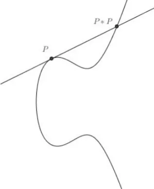
Figure 1.4: The Composition of Two Distinct Points on a Cubic
We can even obtain other rational points knowing only one rational point. IfP
is the rational point we know on the rational cubic, we can draw the tangent line atP, so
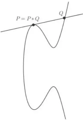
that P is a double root of the cubic equation. Then the third root must also be rational.
Figure 1.5: The Composition of Two Non-Distinct Points on a Cubic
Given any two rational pointsP and Q on a rational cubic curve, we have
de-fined a composition law yielding a third point P∗Q. Does the operation∗acting on the
does not since there is no identity element. Sure, there exists a point Qon a given cubic
curve such that P∗Q=P. Simply draw the tangent to the curve atP and consider the
line as intersecting the curve twice atP.
Figure 1.6: Identity For a Single Point Under ∗
However, in order for Q to be the identity element of the group, for all P0 on
the given cubic, it must be that P0 ∗Q = P0, which is clearly not true. Despite its
shortcomings as a group operation, the composition law∗ is going to play a large role in
the group operation we are going to define. Assume that we know one rational point on
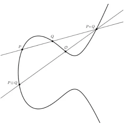
a given non-singular rational cubic curve. Call this pointO. Let⊕be defined as follows:
For two rational points P andQon a non-singular rational cubic
curve, draw a line through P ∗Qand O. The third intersection
Figure 1.7: The Group Operation⊕
Note thatP⊕Qis equivalent toO ∗(P∗Q).
We will be studying specific cubic curves in this paper. We will start by looking
at cubics of the formy2 =x3+ax2+bx+c. This form is calledWeierstrass normal form.
Using projective geometry, one can show that any cubic curve is birationally equivalent to
a Weierstrass equation. The transformations used to put any cubic curve in Weierstrass
form are a homomorphisms. That ensures that the structure of the group law described
above will be preserved. So our study of the group of rational points on a non-singular
rational cubic curve will be reduced to studying rational points on non-singular rational
cubics in Weierstrass form.
For a cubic equation of the form y2 = f(x) = x3 +ax2 +bx+c, if f(x) has
distinct roots, then the curve is called anelliptic curve. Let’s rigorously define an elliptic
curve since it is the basis for the group we will be studying in this paper.
Definition 1.3.1 (Elliptic Curve). An elliptic curve is a nonsingular projective plane
curve E over a field K of degree 3 together with a point O ∈ E(K) that serves as the
We are going to study elliptic curves in Weierstrass normal form using a little
projective geometry. Lettingx= XZ andy= YZ, the homogeneous form of the Weierstrass
curve is
Y2Z =X3+aX2Z+bXZ2+cZ3.
To find the intersection of this curve with the line at infinity, we need to
substi-tute Z = 0 into the equation above. This substitution gives the equation X3 = 0. Thus
X = 0 is a triple root and the cubic has only one point at infinity, the point at which all
vertical lines meet.
We will let the point at infinity be the identity elementO of our group, hence
O is considered rational. So the points on our elliptic curve come from A2∪ {O}. Now
every line will meet the given elliptic curve three times, which you may recall is necessary
for the group operation. The line at infinity will meet the curve three times at O. A
vertical line will intersect the curve at two points in the ordinary affinexy-plane and once
atO. Any other line will intersect the curve three times in the xy-plane, if we allow our
intersections to be complex points.
Given an elliptic curve E, we will denote the group of rational points on E
together with O under the operation ⊕asE(Q). Let’s discuss how ⊕will work for this
group.
Given two points P and Q on E in Weierstrass form, to find P ⊕Q, we start
by drawing the line through P andQ. The third point of intersection is P∗Q. Next, we
draw the vertical line throughP∗Qso that it intersectsO. The third point of intersection
will beP⊕Q. Since all elliptic curves are symmetric about thex-axis, you can also think
about finding P⊕Qby reflecting P∗Qover thex-axis.
Now let’s show that the operation ⊕ together with set of rational points on a
given elliptic curve forms a group.
Theorem 1.3.1. E(Q), where E is a non-singular curve in the projective plane, forms
Proof. Since P∗Q =Q∗P, it is clear thatP ⊕Q=Q⊕P. Thus ⊕is a commutative
operation. We showed earlier that if we have two rational points on a line, it is a rational
line. We also showed that if a rational line intersects a rational cubic curve at two rational
points, then the third intersection is rational as well. So if we start with points P andQ
both rational, then P∗Qwill be rational. SinceOis rational as well, the line through O
and P∗Qis a rational line. HenceP⊕Qis a rational point. Thus the the set of rational
points on a rational cubic is closed under ⊕.
The point at infinity O is the identity element. To verify this, recall P ⊕ O is
equivalent to O ∗(P∗ O), and P ∗ O is the third intersection point of the line through
P and O with the curve. Thus the third point of intersection of the line through P ∗ O
and O is P. So P⊕ O=P and by commutativity, O ⊕P =P as well. Hence O is the
identity element.
Figure 1.8: Verification of Oas the Identity Element
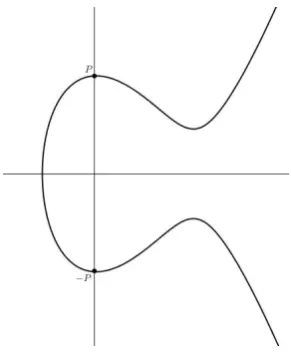
The additive inverse of any point P will be −P such that if P = (x, y), then
−P = (x,−y). To verify this, we need to check thatP⊕(−P) =O. If we connectP and
−P, the vertical line’s third point of intersection withE will be O. Next we will connect
O to O, giving us the tangent line at O which we know intersects E three times at O.
Figure 1.9: The Inverse ofP
Showing that⊕is associative will take some work. First, let’s verify it pictorally
since it is not at all obvious that associativity holds. Let P,Q and R be rational points
on a given rational cubic curve. We want to find (P ⊕Q)⊕R andP ⊕(Q⊕R).
It appears as though (P ⊕Q)∗R is the same point as P ∗(Q⊕R). If that is
true, we are done. For if we adjoin that point to O, the third intersection with the curve
will be (P ⊕Q)⊕R and P ⊕(Q⊕R). So we will prove associativity by proving that
(P⊕Q)∗R=P∗(Q⊕R). In order to do this, we will need the following theorem.
Theorem 1.3.2 (Cayley-Bacharach [ST92, p. 240]). Let C, C1 and C2 be three cubic
curves. Suppose C goes through eight of the nine intersection points ofC1 andC2. Then
C goes through the ninth intersection point.
We have nine points in the figure above–O, P, Q, R, P ∗Q, P ⊕Q, Q∗R,
Q⊕R, and the point at the intersection of `1 and `2, which we will prove lies on the
curve C. A cubic equation can be formed by multiplying three linear equations. So let’s
create the cubic curve C1 by multiplying the equations for the dashed lines and C2 by
multiplying the equations for the solid lines. Then the cubics C1 and C2 pass through
the nine points listed above. We know thatC passes through eight of those points, so by
Theorem 1.6, it must pass through the ninth. Thus (P⊕Q)∗R=P∗(Q⊕R), implying
that (P⊕Q)⊕R=P⊕(Q⊕R). So we have shown associativity. Therefore, the group of
rational points on a non-singular rational cubic curve forms a commutative group under
⊕.
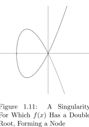
Let’s examine in detail the restriction that our cubic curves be non-singular.
There are two types of singularities that can occur for an cubic curve in normal form
de-pending on the if the point of singularity is a double or triple root off(x). The pictures
for both cases are given in Figure 1.11 and Figure 1.12. For each figure, we have translated
the point of singularity along the x-axis so that is at the origin. The Weierstrass form
Figure 1.11: A Singularity For Which f(x) Has a Double Root, Forming a Node
Figure 1.12: A Singularity For Which f(x) Has a Triple Root, Forming a Cusp
One of the reasons that we have ruled out non-singular curves from our group
is that we already know how to find rational points on them. If we project from the
point of singularity onto a rational line, the line through the point of singularity will
intersect the curve twice at the point of singularity and at one other point. So we get a
one-to-one correspondence between any rational point on the cubic and a rational point
on the rational line. Thus when we have singular points on our curve, we can mimick the
strategy used in Example 1.2.1.
Let’s start with the case for which the point of singularity is a double root of
f(x). For simplicity, let our rational line be x = 1. Since the lines of projection pass
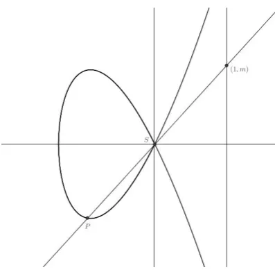
through the origin, they will have the form y = mx. Let S be the point of singularity
and P be the point we are projecting onto x= 1.
We know that P lies on both the elliptic curve and the projection line, so to
Figure 1.13: ProjectingP Onto x= 1
simplifications:
y2 = x2(x+ 1)
m2x2 = x2(x+ 1)
m2 = x+ 1
x = m2−1.
To find they-coordinate ofP, we can substitutex=m2−1 intoy2 =x2(x+ 1):
y2 = x2(x+ 1)
y2 = (m2−1)2·m2
y = m3−m.
Thus for any rational point (1, m) on our rational line, we have a corresponding
rational point (m2−1, m3−m) on our elliptic curve. The choice of the rational linex= 1
was unnecessary since the coordinates of P depends only on the slope of the projection
line, however, it was included here to mimick earlier strategies.
Similarly, for y2 =x3, the case of singularity for which f(x) has a triple root,
Thus, finding the rational points on a singular singular curve is trivial. Also, at
the point of singularity, there is not a distinct tangent line, which makes our geometric
discription of our operation ⊕ problematic. For these reasons, will only discuss elliptic
(non-singular) curves.
1.4
Formulas for the Group Law
We have shown geometrically how to add points in our group. Now we will
develop explicit formulas for adding two points. Let P1 = (x1, y1), P2 = (x2, y2) and
P ∗Q = (x3, y3). We learned above that P⊕Q must have coordinates (x3,−y3). Also,
let the line through P1 and P2 be y = mx+v where m = xy22−−yx11. To find P ∗Q, let’s
substitute y=mx+v intoy2 =x3+ax2+bx+c:
y2 = x3+ax2+bx+c
(mx+v)2 = x3+ax2+bx+c
m2x2+ 2mvx+v2 = x3+ax2+bx+c
0 = x3+ (a−m2)x2+ (b−2mv)x+ (c−v2).
We know thatP1,P2, andP1∗P2 are roots of the equation above, implying that
x3+ (a−m2)x2+ (b−2mv)x+ (c−v2)
= (x−x1)(x−x2)(x−x3)
= x3−(x1+x2+x3)x2+ (x1x2+x1x3+x2x3)x−x1x2x3.
Equating the coefficients of thex2 term givesm2−a=x1+x2+x3. Remember,
our goal was to find P1 ∗P2 = (x3, y3) given (x1, y1) and (x2, y2). We have that x3 =
m2−a−x1−x2. Also, fromy =mx+v, we havey3=mx3+v. Hence, if P1 = (x1, y1),
P2 = (x2, y2) and y=mx+v is the line between them, then
P1⊕P2 = (x3,−y3) = m2−a−x1−x2,−(mx3+v)
. (1.3)
We will have to alter our method slightly if the two given points are the same. If we want
to find P ⊕P or 2P, where P = (x, y), we will need the slope of the tangent line at P.
From implicit differentiation on y2 =f(x) =x3+ax2+bx+cwe have that
2ydy
dx = f
0 (x)
dy dx =
f0(x) 2y .
So the only changes necessary will be that m = f02(yx). By substituting m into
the formula for the x-coordinate of P1⊕P2 and letting x1 and x2 be the same value,x,
we have a formula for the x-coordinate of 2P.
m2−a−2x =
f0(x) 2y
2
−a−2x
= (3x
2+ 2ax+b)2
4x3+ 4ax2+ 4bx+ 4c −a−2x
= x
4−2bx2−8cx+b2−4ac
4x3+ 4ax2+ 4bx+ 4c .
We will denote thex-coordinate of 2P asx(2P). Thus
x(2P) = x
4−2bx2−8cx+b2−4ac
4x3+ 4ax2+ 4bx+ 4c . (1.4)
We will refer to this formula as the duplication formula. Now let’s find the y
-coordinate for 2P or y(2P). From (1.3), we know that the y-coordinate for (x1, y1)⊕
(x2, y2) is−(mx3+v) wherex3 was the resultingx-coordinate upon addition of the given
points. Thus x3 is given by (1.4). Also, y =mx+v implies that v =y−mx. We also
know that for 2P,m= f02(yx). Substitutingm,v and x3 into −(mx3+v), we have
y(2P) = −f02(yx)x4−2bx2−8cx+b2−4ac
4x3+4ax2+4bx+4c
−(y−mx)
= −f
0(x)(x4−2bx2−8cx+b2−4ac)
8y3 −y+
f0(x)x
2y
= −f0(x)[(x2−b)2−8cx8−y34ac]−8y4+4f0(x)xy2
1.5
Properties of Points of Finite Order
We are going to examine some points of finite order since some properties of
these points will be used in later proofs. Another advantage to looking at these points is
that we will become more familiar with our group and some of its algebraic structure.
Definition 1.5.1. An elementP of any group is said to have order m if
mP =P ⊕P⊕ · · · ⊕P
| {z }
msummands
=O,
but m0P 6=O for all integers 1≤m0 < m. If such an m exists, then P hasfinite order;
otherwise it has infinite order.
Let’s prove the following proposition about points of order two and three.
Theorem 1.5.1 (Points of Order Two and Three). Let Ebe the non-singular cubic curve
E:y2=f(x) =x3+ax2+bx+c.
[Recall thatE is non-singular provided f(x) and f0(x) have no common complex roots.]
(a) A point P = (x, y)6=O onE has order two if and only if y= 0.
(b) E has exactly four points of order dividing 2. These four points form a group which
is a product of two cyclic groups of order two.
(c) A point P = (x, y) 6= O on E has order three if and only if x is a root of the
polynomial
ψ3(x) = 3x4+ 4ax3+ 6bx2+ 12cx+ 4ac−b2
.
(d) E has exactly nine points of order dividing 3. These nine points form a group which
is a product of two cyclic groups of order three.
(a) Let P = (x, y) 6= O on E be a point of order two. Then 2P = O, or equivalently
P =−P. If (x, y) = (x,−y), then y= 0.
Suppose conversely that P = (x,0) is onE. From what we know about the shape of
elliptic curves in Weierstrass form, there is a vertical tangent atP. This is supported
by the fact that dxdy = 3x2+22yax+b will result in division by zero forP = (x,0). To find
2P, we draw the vertical tangent to the curve at P, giving us P ∗P = O. Now we
draw the line connecting O to O, the line at infinity, which meets the cubic at the
point O three times. Hence 2P =O.
(b) From above, we know that points of order two have the property y = 0. For
y2 = f(x) = x3 +ax2 +bx+c, the only way y = 0 is if f(x) = 0. Allowing for
complex coordinates, since f(x) is non-singular, it has three distinct roots, say P1,
P2 and P3. So there are three points of order two. The only other point onE with
order dividing 2 is O, the only point of order one. Thus E has exactly four points of
order dividing 2, the set {O, P1, P2, P3}.
Now let’s show that these four points form a group isomorphic to Z2 ⊕Z2. The
identity O is an element of the group. Every element is its own inverse. We can
check for closure and that the group is isomorphic to Z2⊕Z2 by checking that for
any points excluding the identity, the sum of any two points is the third point. It is
clear that any element added to the identity will still be in the group. If we draw the
line through P1 and P2, we have that P1∗P2 =P3. If we draw the line through P3
and O we get a vertical line whose third point of intersection is againP3. Since the
points are colinear, it is clear that if we chose to add any two of the points, we would
get the third. Finally, associativity is inherited from the group. So the set above is
a group isomorphic to the Klein group if we allow complex coordinates. If we allow
only real coordinates, it is either isomorphic to the Klein group or a cyclic group of
order two since we can have three or one real root as depicted in Figure 1.14 and
Figure 1.15. If we allow only rational coordinates, our set is either isomorphic to the
Figure 1.14: f(x) with Three Real Roots
Figure 1.15: f(x) with One Real Root
(c) LetP = (x, y)6=OonE be a point of order three. Then 3P =Oor rather 2P =−P.
Setting the duplication formula equal to x, we have
x4−2bx2−8cx+b2−4ac
4x3+ 4ax2+ 4bx+ 4c = x (1.6)
x4−2bx2−8cx+b2−4ac = 4x4+ 4ax3+ 4bx2+ 4cx
3x4+ 4ax3+ 6bx2+ 12cx+ 4ac−b2 = 0.
Thus x is a root of ψ3 = 3x4+ 4ax3+ 6bx2+ 12cx+ 4ac−b2
.
On the other hand, let P = (x, y)6=O be a point on E such that ψ3(x) = 0. Then
following the sequence of equations above backwards, we have (1.6). That implies
that 2P =P or 2P =−P. If 2P =P, then P =O, which we have excluded. Thus
2P =−P, implying that 3P =O. Therefore, P has order three.
If we set this equal to x, we have
f0(x)2
4f(x) −a−2x = x
f0(x)2−4af(x)−8xf(x)
4f(x) = x
f0(x)2−4af(x)−8xf(x) = 4xf(x)
12xf(x) + 4af(x)−f0(x)2 = 0
2f(x)(6x+ 2a)−f0(x)2 = 0.
Fromf(x) =x3+ax2+bx+c, it follows thatf00(x) = 6x+ 2a. So an alternate form
for ψ3 is
ψ3 = 2f(x)f00(x)−f0(x)2.
Since we are allowing complex coordinates and ψ3 is of degree four, we have four
solutions. To show that they are distinct, we need to show that ψ3(x) and ψ30(x)
have no common roots. We know that ψ3(x) = 2f(x)f00(x)−f0(x)2, from which we
have that
ψ30(x) = 2f(x)f000(x) + 2f0(x)f00(x)−2f0(x)f00(x)
= 2f(x)f000(x)
= 12f(x).
The only way for 2f(x)f00(x)−f0(x)2 and 12f(x) to have a common root is if f(x)
and f0(x) have a common root, but we are given thatf(x) is non-singular. Thus the
four roots of ψ3 are distinct. We showed in (c) that for P = (x, y) 6= O, if x is a
root of ψ3, then 3P =O. So we can conclude that if x1, x2, x3 and x4 are the four
distinct roots of ψ3, then the set
S ={O,(x1,±
p
f(x1)),(x2,±
p
f(x2)),(x3,±
p
f(x3)),(x4,±
p
f(x4))}
is the complete set of points of order dividing three. To show that (xi, yi) are distinct,
we just need to show that yi 6= 0. If yi = 0, from (a), the given point would have
are nine points of order dividing 3. Thus, if we can show that S is a group, then
S ∼=Z3⊕Z3.
We know that S⊆E(C). Let’s use the One-Step Subgroup Test. Letaand bbe any
two distinct points of S of order 3. It follows thata3 =b3 =O. Since S is abelian,
we have that
ab−13
= a3 b−13
= a3 b3−1
= O.
It follows that ab−1 ∈ S since S contains the complete set of elements of order 3.
Therefore, S is a group.
Note that a point on an elliptic curve is an inflection point if and only if 3P =O.
Consider Figure 1.16 below, which shows the group operation for 2P. IfP and −2P were
to collide (or −P and 2P), we would obtain and inflection point as depicted in Figure
1.17, for which it is clear that 3P =O.
Figure 1.16: Finding 2P Figure 1.17: The Collision ofP and
−2P
We will conclude this chapter with an important theorem that we will use later
Theorem 1.5.2 (Nagell-Lutz [ST92, pp. 49-57]). Let
y2=f(x) =x3+ax2+bx+c
be a non-singular cubic curve with integer coefficients a, b, c; and letDbe the discriminant
of the cubic polynomial f(x),
D=−4a3c+a2b2+ 18abc−4b3−27c2.
Let P = (x, y) be a rational point of finite order. Then x and y are integers; and either
Chapter 2
Curves of the Form
y
2
=
x
3
+
ax
2
+
bx
+
c
2.1
Mordell’s Theorem
In 1922, German mathematician Louis Mordell proved the following theorem as
an answer to a question posed by Poincare in 1908.
Theorem 2.1.1 (Mordell’s Theorem). Let E be a non-singular cubic curve given by an
equation
E:y2=x3+ax2+bx+c
where aandbare integers. Then the group of rational pointsE(Q)is a finitely generated
abelian group.
A more general case was proven in 1928 by Andr´e Weil in his dissertation.
Theorem 2.1.2 (Mordell-Weil). Let E be an elliptic curve defined over a number field
K. The group E(K) is a finitely generated Abelian group.
Mordell conjectured that any non-singular projective curve of genus greater than
proved it. Gerd Faltings won a Fields Medal in 1986 for proving Mordell’s conjecture.
By Mordell’s theorem, E(Q) is a finitely generated abelian group. From the
Fundamental Theorem of Abelian Groups,E(Q) is isomorphic to a direct sum of infinite
cyclic groups and finite cyclic groups of order a power of a prime. Thus
E(Q)∼=Z⊕Z⊕ · · · ⊕Z
| {z }
rsummands
⊕Zpv1
1 ⊕Zp
v2
2 ⊕ · · · ⊕Zp
vs
s (2.1)
where each pi is prime, and r is therank of E(Q).
We know from Mordell’s theorem that we can generate all rational points on
an elliptic curve from just a finite set using the group law. So how do we find the set
of generators? At this point, that question cannot always be answered. That is what
makes the study of the group of rational points on elliptic curves so interesting, much is
unanswered. This chapter will culminate with a theorem that provides a formula for the
rank of E(Q). If the rank is zero, then E(Q) is finite. We will show a few examples for
which we can actually find E(Q).
In this chapter, we are going to consider the specific Weierstrass curve y2 =
f(x) =x3+ax2+bx. Recall that using the group law, we only need one rational point on
our elliptic curve to generate other rational points. So we want to make the assumption
that the polynomial f(x) has at least one rational root; this is equivalent to saying that
the curve has at least one point of order two. Let the rational point of order two be P.
Then P = (x0,0). We can translate the curve so that P lies at the origin. Any rational
points found on the translated curve will still be rational after translating back since x0
is rational. Knowing that (0,0) is a solution toE implies thatc= 0. Thus,
E:y2 =f(x) =x3+ax2+bx.
2.2
Some Useful Homomorphisms
Before proving the theorem on the rank ofE(Q), we will need a few propositions.
on the rank of E(Q).
Proposition 2.2.1. Let E andE0 be the elliptic curves given by the equations
E:y2 =x3+ax2+bx and E0:y2=x3+ax2+bx,
where
a=−2a and b=a2−4b.
Let T = (0,0)∈E.
(a) There is a homomorphism φ:E→E0 defined by
φ(P) =
y2
x2,
y(x2−b)
x2
, ifP = (x, y)6=O, T,
O, ifP =O or P =T.
The kernel of φ is{O, T}.
(b) Applying the same process toE0gives a mapφ:E0 →E00. The curveE00is isomorphic
to E via the map(x, y)→ x4,y8. There is thus a homomorphismψ:E0 →E defined by
ψ(P) =
y2
4x2,
y(x2−b)
8x2
, if P = (x, y)6=O, T ,
O, if P =O or P =T .
We will not prove this proposition, but it is worth noting that in order to show
that φ is a homomorphism, it is enough to show that for P1,P2, and P3 on E, if P1⊕
P2⊕P3=O, thenφ(P1)⊕φ(P2)⊕φ(P3) =O. For if this were true, then
φ(P1⊕P2) =φ( P3) = φ(P3) =φ(P1)⊕φ(P2).
Proposition 2.2.2. Letφandψ be the homomorphisms described above. IfP = (x, y)∈
E(Q) where E:y2 =x3+ax2+bx, then (ψ◦φ)(P) = 2P.
Proof. First, note thatc= 0 for E. Thus, formulas (1.4) and (1.5) reduce to
2P =
x4−2bx2+b2
4x3+ 4ax2+ 4bx,
x6+ 2ax5+ 5bx4−5b2x2−2ab2x−b3
8y3
,
forP = (x, y)6=O ∈E. Now,
(ψ◦φ)(x, y) = ψ(φ(x, y))
= ψ
y2 x2,
y(x2−b)
x2 =
y(x2−b)
x2
2
4yx22
2 ,
y(x2−b)
x2 y2 x2 2
−(a2−4b)
8yx22
2 =
x2−2bx2+b2
4y2 ,
x6+ 2ax5+ 5bx4−5b2x2−2ab2x−b3
8y3
Therefore, (ψ◦φ)(P) = 2P.
If we allow complex numbers,φ:E →E0 is onto. Since the focus of this paper
is rational points, we want to know what properties φhas when acting on E(Q).
Proposition 2.2.3 (Properties ofφ:E(Q)→E0(Q)).
(i) O ∈φ E(Q).
(ii) T = (0,0)∈φ E(Q) if and only if b=a2−4b is a perfect square.
(iii) Let P = (x, y) ∈ E0(Q) with x 6= 0. Then P ∈ φ E(Q) if and only if x is the
square of a rational number.
Proof.
(i) Recall thatO is considered rational and is therefore an element ofE(Q). From the
definition ofφ, we can conclude that φ(O) =O. Thus O ∈φ E(Q).
y = 0 into y2 =x3+ax2+bx, we have 0 =x(x2+ax+b). Note that x= 0 is an
impossibility for if x = 0 and y= 0, then φ(x, y) =O, notT. So x2+ax+b= 0.
This only has rational solutions if its discriminant is a perfect square. Thus a2−4b
is a perfect square.
Conversely, if a2−4bis a perfect square, then 0 =x3+ax2+bx=x(x2+ax+b)
has rational zeros other than zero. Hence, there exist (x, y) ∈ E(Q) such that
φ(x, y) = (0,0) =T.
(iii) Let P = (x, y) ∈ E0(Q) with x 6= 0. Assume P ∈ φ E(Q). Then there exists (x, y)∈E(Q) such thatφ(x, y) = (x, y). Thus by the definition ofφ, it follows that
x= yx22 =
y x
2
. Thereforex is the square of a rational number.
Suppose conversely that x = t2 for t ∈ Q∗. We need to show that there exists a
point (x, y)∈E(Q) such thatφ(x, y) =P. Consider the points (x1, y1) and (x2, y2)
where x1 = 12
t2−a+yt, x2 = 12
t2−a−yt, y1 = x1t and y2 = −x2t. Since
t6= 0, we have that x1 and x2 are well defined.
Let’s start by showing that (x1, y1) and (x2, y2) are contained in E(Q). First, we
have that
x1x2 =
1 2
t2−a+y
t
·1 2
t2−a−y
t
= 1 4
(t2−a)2−y
2 t2 = 1 4
(x−a)2− y
2 x = 1 4
x3−2ax2+a2x−y2 x
= 1 4
x3−2ax2+a2x−(x3−2ax2+a2x−4bx)
x
= b.
Also, it is easy to see thatx1+x2 =t2−a. Thus,xi+xbi =
yi xi
2
−afori={1,2},
(x2, y2) are contained in E(Q).
Let’s show thatφ(x1, y1) =φ(x2, y2) = (x, y). We will start with φ(x1, y1). From
y1 =x1t, we have that t= xy11. Thus
y21 x21 =
y1
x1
2
= t2
= x.
Now, notice thatx1−x2 = yt. It follows that
y1(x21−b)
x21 =
x1t(x21−x1x2)
x21
= t(x1−x2)
= t
y t
= y.
Therefore, φ(x1, y1) = (x, y). A similar argument will show thatφ(x2, y2) = (x, y)
as well.
We will now set out to prove that for the map ψ:E0 → E, the index hE(Q) :
ψ E0(Q)
i
≤2t+1, where t is the number of distinct prime factors of b. In the process,
we will introduce a useful map α and describe some of its properties. This map will be
used later in our proof of a formula for the rank of E(Q).
LetQ∗ be the multiplicative group of nonzero rational numbers, and letQ∗2 be
the subgroup of the squares of the elements of Q∗. Also, let α:E(Q)→ Q∗/Q∗2 be the
α(P) =
x (modQ∗2), ifP = (x, y)6=O, T,
1 (mod Q∗2), ifP =O,
b (modQ∗2), ifP =T.
Proposition 2.2.4.
(a) The map α:E(Q)→Q∗/Q∗2 described above is a homomorphism.
(b) The kernel ofαis the imageψ E0(Q). Henceαinduces a one-to-one homomorphism
E(Q)
ψ E0( Q)
,→ Q ∗
Q∗2.
(c) Let p1, p2, . . . , pt be the distinct primes dividing b. Then the image of α is contained
in the subgroup of Q∗/Q∗2 consisting of the elements
{±pε1
1 p
ε2
2 · · ·p
εt
t : each εi equals 0 or 1}.
(d) The index hE(Q) :ψ E0(Q)
i
is at most 2t+1.
Proof.
(a) Let’s use a similar strategy to the one outlined for the proof of Proposition 3.1.3.
That is, we will show that αsends inverses to inverses and that if P1⊕P2⊕P3 =O,
then α(P1)α(P2)α(P3)≡1 (mod Q∗2). For thenα(P1⊕P2) =α(−P3)≡α(P3)−1=
α(P1)α(P2) (modQ∗2).
Let P = (x, y)∈E(Q). Then
α(−P) =α(x,−y) =x≡ 1
x =α(x, y)
−1 =α(P)−1 (mod Q∗2).
Now, let P1 = (x1, y1), P2 = (x2, y2) and P3 = (x3, y3) be elements of E(Q). We
know that if P1⊕P2⊕P3 =O, thenP1,P2 andP3 are colinear. Let y=mx+v be
the line passing through them. Since these points are the intersections of y=mx+v
with E:y2 =x3+ax2+bx, we have
y2 = x3+ax2+bx
(mx+v)2 = x3+ax2+bx
m2x2+ 2mvx+v2 = x3+ax2+bx
0 = x3+ (a−m2)x2+ (b−2mv)x−v2. (2.2)
We also know that since P1,P2 and P3 are roots of (2.2), it follows that
x3+ (a−m2)x2+ (b−2mv)x−v2
= (x−x1)(x−x2)(x−x3)
= x3−(x1+x2+x3)x2+ (x1x2+x1x3+x2x3)x−x1x2x3.
If we equate the final terms, then x1x2x3 =v2 ∈Q∗2. Thus
α(P1)α(P2)α(P3) =x1x2x3 =v2 ≡1 (mod Q∗2).
So we have completed the proof of (a) if the three points given are not O orT. We
will leave it to the reader to verify the other cases.
(b) The kernel of α is all of the elements ofE(Q) that map to 1 modulo Q∗2. From the
definition ofα, we can see that these are the elementsO,Tifbis a perfect square, and
the elements of E(Q) whose x-coordinates are perfect squares. If we apply
Proposi-tion 2.2.3 to ψinstead of φ, it is clear that the imageψ E0(Q) is exactly the points mentioned above. Thus the kernel of α is the image ψ E0(Q).
homomor-phism, by the first isomorphism theorem
imα∼=E(Q)/kerα=E(Q)/ψ(E0(Q)).
Thus α induces a one-to-one homomorphism
E(Q)
ψ E0(Q) ,
→ Q
∗
Q∗2.
(c) If we want to know what the image of α looks like, we just need to analyze the x
-coordinates of points in E(Q). It turns out that if P = (x, y) is on E, thenx = em2
and y= en3 for integersm,nand e, wheree >0 and gcd(m, e) = gcd(n, e) = 1. (For
a derivation of these formulas, see Silverman-Tate pg. 68-69.) Substituting x and y
into the equation for E gives
n
e3
2
= m
e2
3
+am e2
2
+bm e2
n2 = m3+am2e2+bme4
n2 = m m2+ame2+be4.
Ifmandm2+ame2+be4 are relatively prime, then each of them would be a positive
or negative square. Hence x = em2 would be a positive or negative square. Thus
α(P) ≡1 (mod Q∗2), and 1∈ {±pε11p
ε2
2 · · ·pεtt} where the pi are as described above.
If m andm2+ame2+be4 are not relatively prime, then let
d= gcd(m, m2+ame2+be4).
Thenddividesmandbe4. We know thatmandeare relatively prime, thusddivides
b. Now, the primes that dividem but do not divide b must be of even power. The
primes dividing mand b can be of either even or odd power. Thus
m=±(integer)2·pε1
1 p
ε2
2 · · ·p
εt t ,
There-fore,
α(P) =x= m
e2 ≡ ±p
ε1
1 p
ε2
2 · · ·pεtt (modQ
∗2).
If x = 0, then the method above fails. However, ifx = 0, then y = 0 sinceE:y2 =
x3+ax2+bx. Nowα(T) =b(mod Q∗2) and b=±pε11p
ε2
2 · · ·p
εt
t . Thus the image of
α is is contained in the subgroup ofQ∗/Q∗2 consisting of the elements
B ={±pε1
1 p
ε2
2 · · ·p
εt
t : eachεi equals 0 or 1}.
(d) Let’s find the order of the subgroup from (c). Since each power εi can be either 0
or 1, there are two choices for each pεi
i . Thus |{p ε1
1 p
ε2
2 · · ·p
εt
t }|= 2t. Since all of the
elements of the subgroup can be either positive or negative, there are 2(2t) = 2t+1
elements.
We know from (b) that im α ∼= E(Q)/ψ(E0(Q)) and from (c) that im α ⊆ B.
Therefore, the indexhE(Q) :ψ E0(Q)
i
≤2t+1.
2.3
Modules and Exact Sequences
At this point, we will take some time to discuss modules over a ring. We will
use some module theory in future proofs.
Definition 2.3.1. Let R be a commutative ring. An R-module is an additive abelian
groupA together with a functionR×A→A (the image of (r, a) being denoted ra) such
that for all r, s∈R anda, b∈A:
(i) r(a+b) =ra+rb
(ii) (r+s)a=ra+sa
(iii) r(sa) = (rs)a.
(iv) 1Ra=afor all a∈A,
thenAis said to be aunitaryR-module. If Ris a field, then a unitaryR-module is called
a vector space.
It is clear from the definition above that every additive abelian group G is a
unitary Z-module, specifically our group (E(Q),⊕).
Definition 2.3.2. Let A and B be modules over a ring R. A functionf:A→ B is an
R-module homomorphism provided that for all a, c∈Aand r ∈R:
f(a+c) =f(a) +f(c) and f(ra) =rf(a).
Definition 2.3.3. A pair of module homomorphisms, A −→f B −→g C, is said to be exact
at B provided imf=kerg. A finite sequence of module homomorphisms, A0
f1 −→A1
f2 −→
A2
f3
−→ · · ·−−−→fn−1 An−1
fn
−→An, is exact provided imfi =kerfi+1 for i= 1,2, . . . , n−1.
An infinite sequence of module homomorphisms ,· · ·−f−−i−1→Ai−1
f
−→Ai fi+1 −−−→Ai+1
fi+2 −−−→ · · ·
is exact provided imf1 =kerfi+1 for all i∈Z.
Definition 2.3.4. Iff:A→Bis a module homomorphism, thenA/kerf [resp. B/imf]
is called thecoimage [resp. cokernel] of f and is denotedcoimf [resp. cokerf].
Note that from the definitions above, the following claims are true. The
se-quence 0 → A −→f B is an exact sequence if and only if f is a module monomorphism.
Similarly, B −→g C→0 is exact if and only if gis a module epimorphism. If A−→f B−→g C
is exact, then gf = 0 since im f = ker g. Also, if A −→f B −→g C → 0 is exact, then
cokerf =B/imf =B/kerg=coimg∼=C.
Definition 2.3.5. A commutative diagram is a diagram of objects (also known as
ver-tices) and morphisms (also known asarrows oredges) such that all directed paths in the
For example, the diagram below would be commutative ifh◦f =k◦g.
A B
C D
g
f
k
h
Lemma 2.3.1 (Snake Lemma [Lan02, p. 100]). Consider the commutative diagram of
Abelian groups and group homomorphisms below:
A B C 0
0 A0 B0 C0
α f
β g
γ f0 g0
where rows are exact sequences. Then there is an exact sequence relating the kernels and
cokernels of α, β and γ:
kerα→kerβ→kerγ→−δ cokerα→cokerβ →cokerγ.
In order to follow the maps from the statement above, one would have to wind
through the commutative diagram like a snake, as depicted below, giving the lemma its
name.
0 kerf kerα kerβ kerγ
A B C 0
0 A0 B0 C0
cokerα cokerβ cokerγ cokerg 0
f g
α β γ
f0 g0
We can actually extend the Snake Lemma as below.
Lemma 2.3.2 (Extended Snake Lemma). Under the same assumptions as the Snake
Lemma,