A Novel Animal Migration Algorithm for Global Numerical Optimization

A Novel Animal Migration Algorithm for Global

Numerical Optimization

Qifang Luo1_{, Mingzhi Ma}2_{, Yongquan Zhou}2

1 _{College of Information Science and Engineering,}

Guangxi University for Nationalities, Nanning 530006, China [email protected]

2 _{Key Laboratory of Guangxi High Schools Complex System and Computational Intelligence,}

Nanning 530006, China

[email protected], [email protected]

Abstract. Animal migration optimization (AMO) searches optimization solutions by migration process and updating process. In this paper, a novel migration process has been proposed to improve the exploration and exploitation ability of the animal migration optimization. Twenty-three typical benchmark test functions are applied to verify the effects of these improvements. The results show that the improved algorithm has faster convergence speed and higher convergence precision than the original animal migration optimization and other some intelligent optimization algorithms such as particle swarm optimization (PSO), cuckoo search (CS), firefly algorithm (FA), bat-inspired algorithm (BA) and artificial bee colony (ABC).

Keywords: animal migration optimization algorithms, exploration and exploita- tion, functions optimization

1.

Introduction

In recent years, many research have been inspired by animal behavior phenomena for developing optimization techniques, such as firefly algorithm (FA) [1] in 2008, cuckoo search (CS) [2] in 2009, bat algorithm (BA) [2] in 2010, artificial bee colony (ABC) [3] in 2007, monkey algorithm (MA) [4] in 2008, frog-leaping algorithm (SFLA) [5], [6] in 2003. FA mimics flashes of fireflies attract mating partners or potential prey to find optima. CS simulates cuckoos choose a nest where the host bird just laid its own eggs and the first hatched cuckoo evicts the host eggs by blindly propelling the eggs out of the nest. BA simulates the behavior of bats’ echolocation to find food or avoid obstacles by frequency and loudness. And ABC simulates natural bee colony foraging process to search and optimize the objectives by mutual cooperation. Because of its advantages of global, parallel efficiency, robustness and universality, these bio-inspired algorithms have been widely used in constrained optimization and engineering optimization[7], [8], [9], scientific computing, automatic control and other fields [10], [11], [12], [13], [14].

the animals will move to an area with mild climate and abundant food, this is a universal phenomenon exists in nature. The same birds, mammals, fish, reptiles, amphibians, insects and crustaceans all migrate, for example, the reindeer move southward to the taiga to escape from blizzard in winter, and move northward to tundra with rich food in spring. The wildebeest and zebra in Africa move to an area with rich aquatic plants when the rainy season comes, and return back to the usual habitats when the rainy season ends. The white whale, small stripe grain whale and other cetaceans often migrate by following the big fish as their food. The seal, fur seal and other sea mammal animals often climb back to a definite reproduction destination or an ice block to reproduce. In summary, animals like in food rich, water abundant, climatic conditions suitable area for survival, with time goes on, food and water reduce, climate change, living conditions change, the area can no longer provide the needs of the animals to survive, animal population will migrate to a new food and water rich, climatic conditions suitable area. Because of the long difficult journeys, individual animals will leave the migration of population in the process of animal population migration, and also some new individuals will join the migration of population in the process of animal population marching.

2.

Related Work

Biogeography-based optimization is a recently proposed evolutionary algorithm, inspired by the migration behavior of island species [15]. Cuckoo search algorithm is inspired by the obligate brood parasitic behavior of some cuckoo species in combination with the Lévy flight behavior of some birds and fruit flies [16], and applied to classification problem [17], constrained global optimization [18], and various modification version cuckoo algorithm.

Bat Algorithm (BA) is a novel meta-heuristic optimization algorithm based on the echolocation behavior of micro-bats, which was proposed by Xin-she Yang in 2010 [2]. This algorithm is applied to different area. Pei-wei Tsai etc. proposed an improved EBA to solve numerical optimization problems [19]; A multi-objective bat algorithm (MOBA) is proposed by Yang [20], which is first validated against a subset of test functions, and applied to solve multi-objective design problems such as welded beam design. In 2012, BA to solve the Brushless DC wheel motor problem [21].

Animal migration optimization (AMO) algorithm is a novel bio-inspired optimization algorithm by simulating animal migration behavior that proposed by X. Li and J. Zhang in 2013 [22], and applied to clustering analysis [23]. AMO simulates the widespread migration phenomenon in the animal kingdom, through the change of position, replacement of individual, and finding the optimal solution gradually. AMO has obtained good experimental results on many optimization problems.

These algorithms have been applied to various research areas and have gained a lot of success [24], [25], [26], [27], [28]. However, up to new, there is no algorithm that performs well in all the fields. Some algorithms perform much better for some particular problems, while worse for other problems. Until now, how to design a new heuristic algorithm for optimization problem is still open problem [29].

guarantees the MAMO rapid convergence. By means of selecting the better solution space around the current solution, it will improve search ability and accelerate convergence speed, and it has obtained the global optima.

3.

Animal Migration Optimization Algorithm (AMO)

Animal migration algorithm can be divided into animal migration process and animal updating process. In the migration process the algorithm simulates how the groups of animals move from current position to a new position. During this process, each individual should obey three main rules: (1) move in the same direction as its neighbors; (2) remain close to its neighbors; (3) avoid collisions with its neighbors. During the population updating process, the algorithm simulates how animals update by the probabilistic method.

3.1. Animal Migration Process

Fig. 1 The concept of the neighborhood of an animal

During the animal migration process, an animal should obey three rules: (1) avoid collisions with your neighbors; (2) move in the same direction as your neighbors; and (3) remain close to your neighbors. In order to define concept of the local neighborhood of an individual, we use a topological ring, as has been illustrated in Fig. 1. For the sake of simplicity, we set the length of the neighborhood to be five for each dimension of the individual. Note that in our algorithm, the neighborhood topology is static and is defined on the set of indices of vectors. If the index of animal is i then its neighborhood consists of animal having indicesi2,i1, ,i i1,i2, if the index of animal is 1, the neighborhood consists of animal having indicesNP1,NP, 1, 2, 3, etc. Once the neighborhood topology has been constructed, we select one neighbor randomly and update the position of the individual according to this neighbor, as can be seen in Formula (1):

, 1 , ( , , )

i G i G neiborhood G i G

where X_{neiborhood G,} is the current position of the neighborhood,  is produced by using a random number generator controlled by a Gaussian distribution. X_{i G,} is the current position of ith individual, and X_{i G, 1} is the new position of ith individual.

3.2. Population Updating Process

During the population updating process, the algorithm simulates how some animals leave the group and some join in the new population. Individuals will be replaced by some new animals with a probability Pa. The probability is used according to the quality of the fitness. We sort fitness in descending order, so the probability of the individual with best fitness is 1/NP, the individual with worst fitness, by contrast, the probability is 1, and this process can be shown in Algorithm 1.

1. For i1 to NP

2. For j1 to D 3. If randPa

4. Xi G,1Xr G1, rand(Xbest G, Xi G, )rand(Xr2,GXi G, ) 5. End If

6. End For

7. End For

Algorithm 1. Population updating process

1, 2 [1,..., ]

r r  NP are randomly chosen integers, andr₁ r₂ i. After producing the new solutionX_{i G, 1}, it will be evaluated and compared with the X_{i G,} , we choose the individual with a better objective fitness, as can be seen in Formula (2):

, , , 1

, 1

( ) ( )

i G i G i G

i i G

X if f X is better than f X X

X otherwise





  

 (2)

To verify the performance of AMO, 23 benchmark functions were tested. The results show that the proposed algorithm clearly outperforms other evolution algorithms.

4.

The Modified Animal Migration Process

In nature, animals to survive, all animals migrate toward the place with enough food. In this paper, the place is namely living area, and migrating animals have a leader. The proposed modified AMO algorithm established a living area by the leader animal (the individuals with best fitness value) and animals migrate from current locations migrate into this new living area to simulate animal migration process.

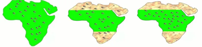
record it. But the amount of food or water gradually diminished as the time wore on, as shown in Fig. 2 (b), some animals migrate from the current areas which have no food and water to a new area with abundant food and water, as shown in Fig. 2 (c). In Fig. 2, the green parts represent the living areas with abundant food and water, animals can live in these areas, and the yellow parts represent the areas that lack of food or water, animals can no longer live in these areas, they must migrate to a new living area (the green parts in Fig. 2 (c)). We shrink the living area after a period of time, as shown in Fig. 2 (a) and (c)), and then animals migrate to the new living area ceaselessly. Because the animals living area is smaller to smaller (by Formula (3) and (4)), after each iteration, the individuals get closer and closer to the best individual, so we can accelerate the convergence velocity and precision of the algorithm to some extent.

(a) The G-th iteration living area (b) Begin to migrate (c) The G1-th iteration living area Fig. 2 Animals migration process

The boundary of the living area is established by

best

lowX R,upX_bestR (3)

R  R (4)

where X_best is the leader animal, low and up are the lower and upper bound of the living area, R is living area radius,  is shrinkage coefficient,  

 

0,1 , low,

up and R are all 1D row vector.

In general, the original value of R depends on the size of the search space. As iterations goes on, a big value of R improves the exploration ability of the algorithm and, a small value of R improves the exploitation ability of the algorithm.

5.

The Modified Animal Migration Optimization Algorithm

(MAMO)

5.1. Initializing the Population

During the initialization process, The algorithm begins by initializing a set of NP

animal positions X X₁, ₂,X₃,...,X_NP,each animal position X_i is a D-dimensional vector containing parameter values to be optimized, such values are randomly and uniformly distributed between the pre-specified lower initial parameter bound a_jand the upper initial parameter bound b_j. So the jth component of the ith vector as Formula (5):

, , [0,1] ( )

i j j i j j j

x a rand  b a ,i1,...,NP, j1,...,D (5)

whererand_{i j,} [0,1] is a uniformly distribution random number between 0 and 1.

5.2. Animals Migration

During the migration process, because animals hunting, foraging or drinking in the living area, some parts of the living area are lack of food or water or climate condition change, some animals migrate from the current living area to the new area which has abundant food and water or climate condition suitable for living. We assume that there is only one living areas, animals out of the new living area would be generated randomly in the new living area, as depicted in Section 3.

5.3. Animals Live Area

During the living process, algorithm simulates individuals’ positions randomly change in living area. Following the biological model, animals hunting, foraging or drinking in habitat, their positions randomly change, an individual move to a new position according to the current position of its neighborhoods, such behavioral rule is move randomly in living area and implemented considering by Formula (1) in Section 2.1.

5.4. Population Updating

1. Begin

2. Set the generation counter G0, living area radius R,

shrinkage coefficient , and randomly initialize with a population of NP animals Xi in solution space

3. Evaluate the fitness for each individual Xi, record the best individual Xbest

4. While stopping criteria is not satisfied do

5. Establish a new living area by lowXbestR,upXbestR 6. Animals migrate into the new living area

7. For 𝑖 = 1 to NP do

8. For 𝑗 = 1 to D do

9. Xi G,1Xi G,  



Xneighborhood G, Xi G,



10. End For

11. End For

12. For i=1 to NP do

13. Evaluate the offspring Xi G,1

14. If Xi G,1 is better than Xi G, then

15. XiXi G,1

16. End If

17. End For

18. For 𝑖 = 1 to NP

19. For 𝑗 = 1 to D

20. Select randomly r1r2i 21. If rand > Pa then

22. Xi G,1Xr G1, rand(Xbest G, Xi G, )rand(Xr2,GXi G, )

23. End If 24. End For

25. End For

26. For 𝑖 = 1 to NP do

27. Evaluate the offspring Xi G,1

28. If Xi G,1 is better than Xi then 29. XiXi G,1

30. End If

31. End For

32. Memorize the best solution achieved so far 33. R R 

34. End while

35. End

6.

Experiments Result and Analysis

In this section, the 23 benchmark test functions have been used to test the performance of the proposed MAMO algorithm. The test functions are classified into 3 different categories:

(1) Unimodal high-dimensional test functions :f₀₁f₀₇. (2) Multimodal high-dimensional test functions:f₀₈f₁₃. (3) Multimodal low-dimensional test functions:

23

14 f

f 

Table 1. Benchmark functions

Benchmark test functions D Range Optimum

2 01 1 ( ) n i i

f x x







30 [-100,100] 0

02 1 1 ( ) | | | | n n i i i i

f x x x

 









30 [-10,10] 0

2 03 1 1 ( ) ( ) n i j i j

f x x

 



 

30 [-100,100] 0

04( ) max | i|,1

f x  x  i n 30 [-100,100] 0

2 2 2 2

05 1

1

( ) [100( ) (1 ) ] n

i i i

i

f x x_ x x







   30 [-30,30] 0

06 1

( ) 0.5

n

i i

f x x







_  _ 30 [-100,100] 0

4 07

1

( ) [0.1)

n i i

f x i x random







  30 [-1.28,1.28] 0

08 1

( ) sin( | |)

n

i i

i

f x x x







  30 [-500,500] -418.9829*n

2 09

1

( ) [ 10 cos 2 10]

n

i i

i

f x x x







  30 [-5.12,5.12] 0

  e x n x n x f n i i n i i                     _{ }   20 2 cos 1 exp 1 2 . 0 exp 20 1 1 2 10 

30 [-32,32] 0

2 11

1 1

1

( ) cos( ) 1

4000 n n i i i i x

f x x

i

 









 30 [-600,600] 0

1

2 2 2 2

12 1 1

1 1

( ) 10sin ( ) ( 1) 1 10sin ( ) ( 1) ( ,10,100,4)

D D

i i D i

i i

f x y y y y u x

D  _  _     _{ }   _ 



    _



1 1 4 i i x y   

( )

( , , , ) 0

( ) m i i i i m i i

k x a x a

u x a k m a x a

k x z x a

  



   

   



30 [-50,50] 0

1

2 2 2 2

13 1 1

1 1

( ) 0.1 10sin ( ) ( 1) 1 10sin ( ) ( 1) ( ,10,100,4)

D D

i i D i

i i

f x y y y y u x





 

 _{ } 

1 25 14 2 6 1 1 1 1 ( )

500 j _{( )}

i ii i

f x

j x a             _{ }        2 [-65.53, 65.53] 0.998004 2 2 11 1 2 15 2

1 3 4

( )

( ) i i

i

i i i

x b b x

f x a

b b x x



  

 _  _

 

 



4 [-5,5] 0.0003075

2 4 6 2 4

16 1 1 1 1 2 2 2

1

( ) 4 2.1 4 4

3

f x  x  x  x x x  x  x 2 [-5,5] -1.0316285

2 2

17 2 2 1 1 1

5.1 5 1

( ) ( 6) 10(1 ) cos 10

8 4

f x x x x x

 



       2 [-5,10]*

[0,15] 0.398

2 2 2

18( ) [1 (1 2 1) (19 141 31 142 61 2 3 )]2 f x   x x  x x  x  x x  x

2 2 2

1 2 1 1 2 1 2 2

[30 (2x 3 ) (18 32x x 12x 48x 36x x 27 )]x

        2 [-5,5] 3

4 3

2 19

1 1

( ) iexp ij( j ij)

i j

f x c a x p

 

 

  _  _

 





3 [0,1] -3.8628

4 6

2 20

1 1

( ) iexp ij( j ij)

i j

f x c a x p

 

 

  _  _

 





6 [0,1] -3.3224







5 1

21 1

( ) i i T i

i

f x X a X a c





 

 



_    _ 4 [0,10] -10.1532







7 1

22 1

( ) i i T i

i

f x X a X a c





 

 



_    _ 4 [0,10] -10.4029







10 1

23 1

( ) _{i i} T _i

i

f x X a X a c





 

 



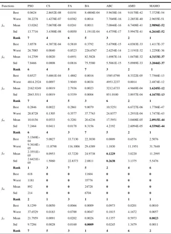
_    _ 4 [0,10] -10.5364

The mean and standard deviation results of 25 independent runs for each algorithm have been summarized in Tables 2, 3 and 4.

6.1. Experimental Setup

All of the algorithms were programmed in MATLAB R2008a, numerical experiment was set up on AMD Athlon(tm)II *4 640 processor and 2GB memory.

6.2. Parameters Setting

We initialize D-dimensional row vector R 



b_ja_j



, j



1, 2,...,D



, a_j and

j

b are the lower bound and upper bound of the solution space. the population size NP

is 50. The maximum numbers of iterations are 1500 for

f

₀₁

,

f

₀₆

,

f

₁₀

,

f

₁₂ and f13,

2000 for

f

₀₂ and

f

₁₁, 3000 for

f

₀₇

,

f

₀₈ and

f

₀₉, 5000 for

f

₀₃

,

f

₀₄ and

f

₀₅,

400 for

f

₁₅, 100 for

f

₁₄

,

f

₁₆

,

f

₁₇

,

f

₁₉

,

f

₂₁

,

f

₂₂ and

f

₂₃, 30 for

f

₁₈, and 200 for

20

Different test functions have different iterations, shrinkage coefficientfor all test functions should be changed according to the each number of iteration to get a living area with same size at the end of iteration. In order to set a unified model to define , Numerical experiments results showed that MAMO algorithm can achieve more ideal effect if we choose the parameter values  = 0.99 for iteration iter=2000, and the final living area radius R_final= 0.992000 =1.8638E-09 (by Algorithm 2) which is small enough to gather the individuals into the living area. We set thisR_finalas standard to set other. An empirical model has been developed by following equation:

2000 0.99iter

  (6)

whereis shrinkage coefficient,iteris the number of iteration.

6.3. Comparison of MAMO with PSO, CS, FA, BA, ABS, and AMO

To demonstrate that the MAMO algorithm’s performance, we compared MAMO with FA [1], CS [2], BA [3], ABC [4], AMO [22], PSO [28], respectively using the best, worst, mean and standard deviation value to compare their performance. The setting values of algorithm control parameters of the mentioned algorithms are given below.

FA: according to [1],  ₀ 0.5, ₀ 0.2 and  1.0, the population size is 100. CS: according to [2], 1.5, Pa0.25, the population size is 50, because of this algorithm has two phases.

BA: according to [3], loudnessA0.25, pulse rate r0.5, 0.95,  0.5, the population size is 50, because of this algorithm has two phases.

ABC: according to [4], limt5D, the population size is 50, because of this algorithm has two phases.

AMO: according to [22], the population size is 50, because of this algorithm has two phases.

PSO: according to [28], weight factor  linear decrease from 0.9 to 0.4,

1 2 1.49445

c c  . The population size is 100.

Unimodal High-dimensional Functions Test Results and Analysis. In the

experiments, the mean results of 25 independent runs for f01f07 _{are listed in Table 2.}

Table 2. Experiment results of benchmark functionsf01f07for different algorithms

Functions PSO CS FA BA ABC AMO MAMO

f01

Best 0.0624 2.8652E-08 0.0191 8.4804E-04 5.9638E-16 9.0170E-42 7.3729E-54 Worst 38.2278 1.4278E-07 0.0382 0.0014 7.7049E-16 2.2853E-40 2.9655E-51 Mean 13.0262 7.0670E-08 0.0261 0.0011 7.0846E-16 6.7408E-41 2.9896E-52

Std 13.7716 3.4388E-08 0.0050 1.1911E-04 4.4759E-17 5.9947E-41 6.2616E-52

Rank 7 4 6 5 3 2 1

f02

Best 3.8578 4.3873E-04 0.5810 0.3792 5.6790E-15 4.0383E-33 1.4117E-37 Worst 26.7085 0.0040 0.8523 226.6767 2.6254E-14 2.1191E-32 1.2250E-36

Mean 14.2709 0.0020 0.6951 82.5828 1.6987E-14 1.0470E-32 4.3153E-37

Std 7.8466 0.0008 0.0816 75.5580 5.5061E-15 5.0989E-33 3.2046E-37

Rank 6 4 5 7 3 2 1

f03

Best 0.8527 5.6861E-04 1.4882 0.0016 1585.0790 8.3322E-05 7.7566E-13

Worst 4814.2524 0.0097 3.9049 0.0034 4953.2237 0.0014 2.4874E-12

Mean 2162.9249 0.0019 2.7936 0.0023 3212.6733 4.9669E-04 1.6245E-12

Std 2043.5511 0.0019 0.5359 0.0004 851.0100 3.8937E-04 4.1675E-13

Rank 7 4 5 3 6 2 1

f04

Best 0.2846 0.0022 0.2861 9.0079 10.5251 6.6727E-06 1.7786E-47

Worst 20.8728 0.1305 0.3577 37.7763 24.8377 1.2931E-04 1.7475E-43

Mean 10.0156 0.0533 0.3281 20.6236 17.5951 3.0408E-05 2.0915E-44

Std 7.2464 0.0411 0.0178 8.3156 4.2192 2.6094E-05 4.5596E-44

Rank 6 4 3 7 5 2 1

f05

Best 5.1569E+

04 5.0827 33.7130 22.3030 0.0009 0.6576 2.5076

Worst 9.3616E+ ₀₅ 11.8798 116.1006 29.4389 1.1830 11.1951 31.7648

Mean 2.3551E+

05 8.0953 43.7220 24.9738 0.1229 3.0220 11.2995

Std 2.6421E+ ₀₅ 1.5060 22.8373 2.0811 0.2638 3.1375 5.5476

Rank 1 3 7 5 2 4 6

f06

Best 618 0 0 11604 0 0 0

Worst 1181 0 0 35776 0 0 0

Mean 892 0 0 24728 0 0 0

Std 214 0 0 6704 0 0 0

Rank 2 1 3 1 1 1 1

f07

Best 8.1299 0.0050 0.0066 0.0009 0.0973 0.0201 0.0010

Worst 37.6529 0.0183 0.0788 0.0047 0.1815 4.1672 0.0057

Mean 21.7959 0.0091 0.0202 0.0026 0.1357 0.5973 0.0023

Std 9.7284 0.0028 0.0160 0.0009 0.0245 1.3479 0.0011

Rank 7 5 3 1 4 6 2

better than MAMO; the PSO is the worst for most functions. For f₀₁, the mean and standard deviation value of MAMO are 2.9896E-52 and 6.2616E-52 respectively which are 9 orders of magnitude better than AMO. The mean value of CS and ABC are 7.0670E-08 and 7.0846E-16. For f02, the best solution that MAMO, AMO and ABC give are 1.4117E-37, 4.0383E-33 and 5.6790E-15, and the standard deviation value of MAMO is more better. For

03

f andf₀₄, MAMO provides the outstanding solution, and the means of MAMO are at least 8 and 39 orders of magnitude better than AMO and other algorithms. For

05

f , the mean value of MAMO and AMO are 3.0220 and 11.2995 respectively, while ABC gives a better solution 0.1229. For

07

f , The mean value of

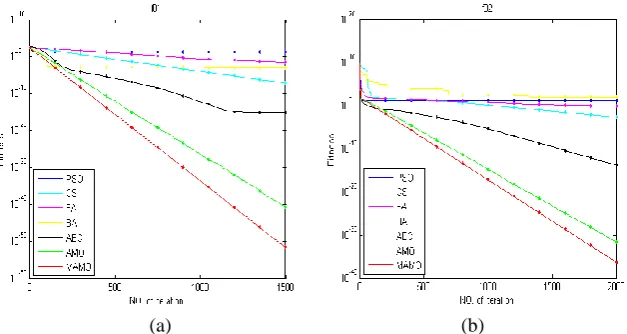
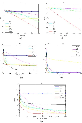
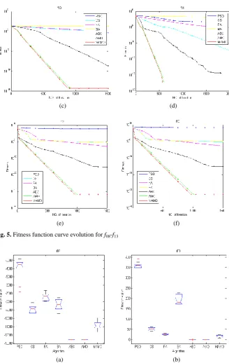
MAMO is 0.0023 which is better than other algorithms. Fig.3 (a-g) shows that the fitness function curve evolution of each algorithm for f₀₁to_f07. These figures show that MAMO has faster convergence rate and the higher optimizing precision in solving multidimensional unimodal functions. Fig.4 (a-g) shows that the graphical analysis results of the ANOVA tests. As can be seen in Fig. 4, when solving function f₀₁ to

07

f , most of the algorithms can obtain the stable optimal value after 25 iteration except PSO algorithm.

Multimodal High-dimensional Functions Test Results and Analysis. For multimodal functions f08-f13, in contrast to unimodal, have many local minima/maxima which are, in general, more difficult to optimize. The final results are more important because of this function can reflect the algorithm’s ability to escape from local optima and obtain the global optimum. We have tested the experiments on f08-f13 where the number of local minima increases exponentially as long as the dimension of the function increases. Table 3 summarizes the best value, the worst value, mean value and the standard deviation value results of 25 independent runs for the selected functions. Generally, we use the index StdDev measure the performance of the algorithm.

(c) (d)

(e) (f)

(g)

(a) (b)

(c) (d)

(g)

Fig. 4. ANOVA tests for f01-f07

Table 3. Experiment results of benchmark functionsf08f13for different algorithms

Functions PSO CS FA BA ABC AMO MAMO

f08

Best -6794.0585 -9447.6445 -7947.6445 -9391.2125 -12569.4866 -12569.4866 -11760.1553 Worst -2753.3192 -7433.8598 -5933.8598 -6587.5532 -12569.4866 -12569.4866 -9430.7862 Mean -3597.9022 -8754.0246 -7234.9052 -8169.9329 -12569.4866 -12569.4866 -10755.3884

Std 897.3297 591.0898 553.2876 761.6005 1.0668E-07 4.0674E-13 600.5346

Rank 7 4 3 6 2 1 5

f09

Best 331.8060 34.4147 12.6914 131.4967 0 0 7.9597

Worst 402.7944 67.2098 45.5377 232.0392 3.4106E-13 0 32.8336

Mean 365.0584 52.2082 23.9947 190.2430 8.8107E-14 0 17.6108

Std 17.1292 9.0984 6.4741 30.3222 8.1338E-14 0 5.5406

Rank 6 5 4 7 2 1 3

f10

Best 16.7332 0.0263 0.3164 15.7627 2.9885E-10 4.4409E-15 4.4409E-15

Worst 19.7878 1.3344 0.4961 19.2294 4.3636E-09 4.4409E-15 4.4409E-15

Mean 18.2910 0.4648 0.4186 18.0883 1.9940E-09 4.4409E-15 4.4409E-15

Std 0.7456 0.4337 0.0465 0.8667 1.1632E-09 0 0

Rank 5 4 3 6 2 1 1

f11

Best 29.2946 9.34444E-09 0.8163 379.8683 0 0 0

Worst 108.3321 2.14236E-07 0.9571 1954.0418 3.7526E-14 0 0

Mean 57.2072 4.59672E-08 0.9008 1354.8913 2.9143E-15 0 0

Std 15.6863 4.40214E-08 0.0379 492.8702 8.1411E-15 0 0

Rank 5 3 4 6 2 1 1

f12

Best 1.3873E+07 0.0700 0.0014 0.0372 4.6085E-16 1.5705E-32 1.5705E-32

Mean 6.9715E+07 0.4865 0.0020 0.5112 6.5351E-16 1.5705E-32 1.5705E-32

Std 5.5922E+07 0.2755 0.0003 0.2857 8.4555E-17 2.7369E-48 2.7369E-48

Rank 3 5 4 6 2 1 1

f13

Best 5.5425E+07 0.0426 0.0012 0.0054 3.7274E-16 1.4998E-32 1.4998E-32

Worst 3.4650E+08 1.1267 0.0023 1.2763 7.7667E-16 1.4998E-32 1.4998E-32

Mean 1.8237E+08 0.4748 0.0019 0.6838 6.7482E-16 1.4998E-32 1.4998E-32

Std 8.1652E+07 0.2814 0.0003 0.3803 1.1951E-16 5.4738E-48 5.4738E-48

Rank 3 5 4 6 2 1 1

As can be seen rank line in Table 3, for test functions f₀₈f₁₃, most of the solutions

of MAMO and AMO get similar solution except

f

₀₈ and

f

₀₉. For

f

₀₈ and

f

₀₉,

AMO achieves the optimal value. For

f

₁₀ to

f

₁₃, AMO and MAMO provide the same best mean and standard deviation value of all algorithms. For

f

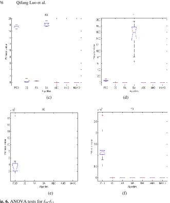
₁₀, the best, worst, mean and standard deviation value of AMO and MAMO are all 0. Fig. 5 (a-f) shows the fitness function curve evolution. From Fig. 6, we can conclude that although MAMO and AMO converge to the same value, MAMO has a faster convergent rate than AMO when solving

f

₁₀

,

f

₁₁

,

f

₁₂ and

f

₁₃. Fig. 6 (a-f) shows the graphical analysis results of the ANOVA tests.

(c) (d)

(e) (f)

Fig. 5. Fitness function curve evolution for f08-f13

(c) (d)

(e) (f)

Fig. 6. ANOVA tests for f08-f13

Multimodal Low-dimensional Functions Test Results and Analysis. For multimodal low-dimensional functions f14-f23, they have only a few local minima and the dimension of the function is also small, so we use lower iterations to compare MAMO with other algorithms. In the experiment, the mean results of 25 independent runs are summarized in Table 4. Generally, we use the index StdDev measure the performance of the algorithm.

Table 4. Experiment results of benchmark functions f14-f23 for different algorithms

Functions PSO CS FA BA ABC AMO MAMO

f14

Best 0.99801 0.99800 0.99800 0.99800 0.99800 0.99800 0.99800

Worst 499.80461 0.99800 0.99800 0.99800 0.99800 0.99800 0.99800

Std 189.27530 2.2067E-12 1.1764E-10 1.0066E-15 1.1827E-11 2.1642E-13 1.9860E-16

Rank 7 4 6 2 5 3 1

f15

Best 0.00113 0.00052 0.00051 0.00031 0.00064 0.00032 0.00031

Worst 0.00527 0.00105 0.00159 0.00159 0.00153 0.00049 0.00072

Mean 0.00289 0.00084 0.00098 0.00081 0.00099 0.00041 0.00057

Std 0.00127 0.00013 0.00030 0.00030 0.00020 4.5475E-05 0.00014

Rank 6 2 5 5 4 1 3

f16

Best -1.03150 -1.03163 -1.03163 -1.03163 -1.03163 -1.03163 -1.03163

Worst -1.02072 -1.03163 -1.02915 -1.03163 -1.03161 -1.03163 -1.03163

Mean -1.02929 -1.03163 -1.03148 -1.03163 -1.03163 -1.03163 -1.03163

Std 0.00268 1.4305E-07 0.00053 1.1850E-07 3.8469E-06 1.4745E-11 2.9790E-16

Rank 7 4 6 3 5 2 1

f17

Best 0.39899 0.39789 0.39789 0.39789 0.39789 0.39789 0.39789

Worst 2.30267 0.39796 0.39798 0.39789 0.39790 0.39789 0.39789

Mean 0.82386 0.39790 0.39791 0.39789 0.39789 0.39789 0.39789

Std 0.51750 1.5795E-05 2.1140E-05 5.2758E-08 3.6487E-06 0 0

Rank 6 4 5 2 3 1 1

f18

Best 3.08497 3.00977 3.00088 0.39789 3.02122 3.00100 3

Worst 12.15882 5.63852 3.03221 0.39789 18.07006 3.03955 3

Mean 5.18553 3.44519 3.01060 0.39789 5.37064 3.00902 3

Std 2.24017 0.77291 0.00878 5.2758E-08 3.94782 0.01072 1.5132E-14

Rank 6 5 3 2 7 4 1

f19

Best -3.85076 -3.86278 -3.86278 -3.86278 -3.86278 -3.86278 -3.86278

Worst -3.02071 -3.86267 -3.86099 -3.86274 -3.86031 -3.86278 -3.86278

Mean -3.60090 -3.86277 -3.86258 -3.86277 -3.86266 -3.86278 -3.86278

Std 0.22133 2.3902E-05 0.00051 9.0408E-06 0.00054 1.6347E-15 1.9885E-16

Rank 7 4 5 3 6 2 1

f20

Best -2.62396 -3.32214 -3.32234 -3.32219 -3.32237 -3.32207 -3.32237

Worst -1.50458 -3.31778 -3.15394 -3.20192 -3.32235 -3.32206 -3.32237

Mean -2.00192 -3.32126 -3.27488 -3.25630 -3.32237 -3.32207 -3.32237

Std 0.30426 0.00106 0.06519 0.05936 3.4784E-06 1.9844E-06 9.9711E-08

Rank 5 4 7 6 3 2 1

Worst -2.16927 -9.24270 -2.68018 -2.63045 -9.39489 -8.27469 -2.63047

Mean -4.49265 -9.79876 -8.33948 -5.90740 -10.04447 -10.01521 -8.40389

Std 1.11378 0.23143 3.12530 3.53661 0.18117 0.41829 3.14839

Rank 4 2 5 7 1 3 6

f22

Best -5.08767 -10.37347 -10.40096 -10.40293 -10.40287 -10.40294 -10.40294

Worst -1.58721 -9.51770 -10.37968 -2.75189 -9.81857 -10.09594 -10.40294

Mean -4.48409 -9.97271 -10.39251 -5.48586 -10.30291 -10.38664 -10.40294

Std 1.21181 0.24158 0.00615 2.61886 0.15940 0.06672 3.4628E-15

Rank 6 5 2 7 4 3 1

f23

Best -5.12847 -10.45131 -10.53431 -10.53604 -10.53625 -10.53641 -10.53641

Worst -2.85665 -7.22276 -10.49722 -2.42733 -9.67901 -10.40656 -10.53641

Mean -4.57954 -9.71234 -10.52331 -6.04331 -10.33162 -10.52719 -10.53641

Std 0.73895 0.77320 0.01074 3.36106 0.24255 0.02931 9.9823E-16

Rank 5 6 2 7 4 3 1

From rank line in Table 4, we can seen the best, worst, mean and standard deviation value of MAMO algorithm are superior when solving the multimodal low-dimensional functions. For

f

₁₄, results of all algorithms except PSO approximate to the optimal value 0.99800, while the standard deviations of MAMO is 1.9860E-16, which is better than 2.2067E-12, 1.1764E-10, 1.0066E-15, 1.1827E-11, 2.1642E-13 that obtained respectively by CS, FA, BA, ABC, AMO. For f₁₅, the most solutions of the algorithms are in the same order of magnitude, but the solution of AMO is more approximate to the optimum value. For polynomial functions

f

₁₆,

f

₁₇ and

f

₁₈, the mean of most of the algorithms achieve the same order of magnitude, but the mean value of MAMO are -1.03163, 0.39789 and 3 which all reached the globally optimal solution. For

19

f

and

f

₂₀, the best, worst and the mean value are all -3.86278 and -3.32237

(a) (b)

(c) (d)

(g) (h)

(i) (j)

Fig. 7. Fitness function curve evolution for f14-f23

(c) (d)

(e) (f)

(i) (j)

Fig. 8. ANOVA tests for f14--f23

7.

Evaluation of Living Area Radius

The performance and results of the proposed algorithms are greatly affected by the size of living area, a big value of Rcan provide a big solution space, which could enhance the diversity of individuals, and a small value of R can fast gather the individuals around the best individual. We adopted different shrinking coefficientto change the living area radius after each iteration, as shown in Formula (3) and (4), and set a unified

model 0.992000iter in Formula (6). To study the extent of R impacts on the proposed

algorithm, we selected one unimodal high-dimensional function and one multimodal high-dimensional function separately, set differentto evaluate the proposed algorithm.

Fig. 9 (a) shows the results of an experiment on

f

₀₁, we can conclude that if we choose0.90, it has a better convergence precision than0.93, 0.96,

0.99

 , while if we choose0.85and0.80, MAMO algorithm plunges into

local optima. So the bestfor

f

₀₁must exist between 0.85 and 0.90. And likewise in

Fig. 9 (b), for

f

₁₁, MAMO algorithm quickly converged at global optimum before 400 iterations if we choose0.99,0.96or0.93, while MAMO could not escape from poor local optima and to global optimum if we choose0.90,0.85or

0.80

(a) (b)

Fig. 9. Fitness function curve evolution for

f

₀₁and

f

₁₁with different

8.

Conclusions

In this paper, to improve the deficiencies of the AMO algorithm, we modified the algorithm by using a new migration method. By 23 benchmark test functions, include unimodal high-dimensional, multimodal high-dimensional and multimodal Low-dimensional functions, we provide some comparisons of MAMO with PSO, CS, FA, BA, ABS, AMO and an experimental results show that MAMO algorithm has strong global searching ability and local optimization ability, MAMO has improved the convergence speed and convergence precision of AMO, therefore, it is very effective to solve complex functions optimization problems. At last, how to define a proper and unified radius of living area need to be considered in subsequent work.

Acknowledgments. This work is supported by National Science Foundation of China under Grants No. 61463007, 61563008. Key Project of Guangxi University Science Foundation under Grant No. 2012MDZD037.

References

1. Yang, X. S.: Nature-Inspired Metaheuristic Algorithms. Luniver Press, New York, USA. (2008)

2. Yang, X. S.: Deb S. Cuckoo search via Levy flights, In Proceedings of World Congress on Nature & Biologically Inspired Computing (NaBIC 2009). IEEE Publication, New York, USA, 210-214. (2009)

3. Karaboga, D., Basturk, B.: A powerful and efficient algorithm for numerical function optimization: Artificial Bee Colony (ABC) algorithm. J Global Optim, Vol. 39, No. 3, 459-471. (2007)

5. Eusuff, M., Lansey, K.: Optimization of water distribution network design using the shuffled frog leaping algorithm. Journal of Water Resources Planning and Management, Vol. 129, No.3, 210-225. (2003)

6. Eusuff, M., Lansey, K., Pasha, F.: Shuffled frog-leaping algorithm: a memetic meta-heuristic for discrete optimization. Engineering Optimization, Vol. 38, No. 2, 129-154. (2006)

7. Passino, K.: Biomimicry of Bacterial Foraging for Distributed Optimization and Control. IEEE Control Systems Magazine, Vol. 22, No.3, 52-67. (2002)

8. Gandomi, A., Yang, X. S., Alavi, A., Talatahari, S.: Bat algorithm for constrained optimization tasks. Neural Comput & Applic, Vol. 22, No.6, 1239–125.(2013)

9. Andomi, A., Yang, X. S., Alavi, A .: Cuckoo search algorithm: a metaheuristic approach to solve structural optimization problems. Eng Comput,Vol.29, No.1, 17-35 (2013)

10. Mohan, B., Baskaran, R.: Energy aware and energy efficient routing protocol for adhoc network using restructured artificial bee colony system. Commun Comput Inf Sci, Vol. 169, No. 3, 473-484. (2011)

11. Clerc, M., Kennedy, J.: The particle swarm-explosion, stability, and convergence in a multidimensional complex space. IEEE Trans Evol Comput, Vol. 6 , No.1,58-73. (2002) 12. Horn, J., Nafpliotis, N., Goldberg, D. E.: A niched Pareto genetic algorithm for

multiobjective optimization. Evol Comput, Vol. 1, No.1, 82-87. (1994)

13. Rao, R., Patel, V.: Optimization of mechanical draft counter flow wet-cooling tower using artificial bee colony algorithm. Energy Convers Manage, Vol. 52, No. 7, 2611-2622. (2011) 14. Karaboga, D., Ozturk, C., Karaboga, N., Gorkemli, B.: Artificial bee colony programming

for symbolic regression. Inf. Sci, Vol. 209, 1-15. (2012)

15. Simon, D.: Biogeography-Based Optimization. IEEE Trans Evol Comput, Vol. 12, No. 6, 702-713. (2008)

16. Yang, X. S., Deb, S.: Engineering Optimization by Cuckoo Search. Int J Math Model Numer Optim. Vol. 1, No. 4, 330-343. (2010)

17. Goel, S., Sharma, A., Bedi, P.: Novel Approaches for Classification Based on Cuckoo Search Strategy. International Journal of Hybrid Intelligent Systems, Vol. 10, No.3,107-116. (2013)

18. Long, W., Liang, X.M., Huang, Y.F., Chen, Y.X.: An effective Hybrid Cuckoo Search Algorithm for Constrained Global Optimization. Neural Computing and Applications, Vol. 25, No.3, Springer Ver-lag, 911-926. (2014)

19. Tsai, P. W.: Bat Algorithm Inspired Algorithm for Solving Numerical Optimization Problems. Applied Mechanics and Materials, Vol.148-149, Elsevier Science, 134-137.(2011)

20. Yang, X. S.: Bat Algorithm for Multi-objective Optimization. International Journal of Bio-Inspired Computation Bio-Bio-Inspired Computation, Vol. 3, No. 5, 267-274. (2011)

21. Bora, T. C., Coelho, L. S., Lebensztajn, L.: Bat-Inspired Optimization Approach for The Brushless DC Wheel Motor Problem. IEEE Transactions On Magnetics, Vol. 48, No. 2, 947-950. (2012)

22. Li, X., Zhang, J., Yin, M.: Animal Migration Optimization: an optimization algorithm inspired by animal migration behavior. Neural Computing and Applications, Vol. 24, No.7, 1967-1877. (2014)

23. Ma, M. Z., Luo, Q. F., Zhou, Y. Q., Chen, X., Li, L. L.: An Improved Animal Migration Optimization Algorithm for Clustering Analysis. Discrete Dynamics in Nature and Society, Vol. 2015, Hindawi Publishing Corporation, Article ID 194792, 1-12. (2015)

24. Walton, S., Hassan, O., Morgan, K., Brown, M. R.: Modified Cuckoo Search: A New Gradient Free Optimization Algorithm. Chaos Solitons Fractals, Vol. 44, 710-718. (2011) 25. Yang, X. S.: A New Metaheuristic Bat-Inspired Algorithm. Studies in Computational

Intelligence, Vol. 284, Springer Ver-lag,65-74(2010)

27. Li, X, Wang, J, Zhou, J, Yin, M.: A Perturb Biogeography Based Optimization with Mutation for Global Numerical Optimization. Appl Math Comput. Vol. 218, No. 2, 598-609. (2011)

28. Eberhart, R., Kennedy J.: A new optimizer using particle swarm theory. In Proceedings of the Sixth Int. Symposium on Micromachine and Human Science. Springer-Verlag, Berlin Heidelberg New York, Nagoya, Japan. 39-43. (1995)

29. Wolpert, D. H., Mcready, W. G.: No Free Lunch Theorems for Optimization. IEEE Trans Evol Comput. Vol. 1, No.1, 67-82.(1997)

Qifang Luo, Associate Professor. She received the MS degree in computer science from Guangxi University in 2005, Her research interests are in the areas of computation intelligence, and intelligence information systems.

Mingzhi Ma, M.S., received the BS degree from College of Information Science and Engineering, Guangxi University for Nationalities, China, in 2015. His current research interest is in computation intelligence, swarm intelligence algorithm.

Yongquan Zhou, Ph.D & Prof, received the MS degree in computer science from Lanzhou University, Lanzhou, China, in 1993 and the PhD degree in computation intelligence from the Xiandian University, Xi’an, China, in 2006. He is currently a professor at Guangxi University for Nationalities. His research interests include computation intelligence, neural networks, and intelligence information processing.