A Longitudinal Adoption Study of Substance Use Behavior in Adolescence

(1)

A Longitudinal Adoption Study of Substance Use

Behavior in Adolescence

Brooke M. Huibregtse,1,2_{Robin P. Corley,}1_{Sally J. Wadsworth,}1_{Joanna M. Vandever,}1,2 John C. DeFries,1_{and Michael C. Stallings}1,2

1_{Institute for Behavioral Genetics, University of Colorado Boulder, Boulder, Colorado, USA}

2_{Department of Psychology and Neuroscience, University of Colorado Boulder, Boulder, Colorado, USA}

Although cross-sectional twin studies have assessed the genetic and environmental etiologies of sub-stance use during adolescence and early adulthood, comparisons of results across different samples, measures, and cohorts are problematic. While several longitudinal twin studies have investigated these issues, few corroborating adoption studies have been conducted. The current study is the first to estimate the magnitude of genetic, shared environmental, and non-shared environmental influences on substance use (cigarettes, alcohol, and marijuana) from ages 14 to 18 years, using a prospective longitudinal adoption design. Adoptive and control sibling correlations provided substantial evidence for early genetic effects on cigarette, alcohol, and marijuana use/no use. Shared environmental effects were relatively modest, except for alcohol use, which showed increases in late adolescence (age 17 to 18 years). Sibling similarity for quantity/frequency of use also support additive genetic influences across adolescence, with some shared environmental influences for all three substances. To test the stability of these influences across time, a series of independent pathway models were run to explore common and age-specific influences. For all substances, there were minimal age-specific additive genetic and shared environmental influences on quantity/frequency of use. Further, there was a trend toward increasing genetic influences on cigarette and alcohol use across ages. Genetic influences on marijuana were important early, but did not contribute substantially at age 17 and 18 years. Overall, the findings indicate that genetic influences make important contributions to the frequency/quantity of substance use in adolescence, and suggest that new genetic influences may emerge in late adolescence for cigarette and alcohol use.

Keywordscigarettes, alcohol, marijuana, adoption, longitudinal

The transition from adolescence into adulthood is a par-ticularly formative period for a number of behaviors. In the case of substance use, both initial experimentation and continued use are thought to be due to a combination of genetic and environmental influences. Similar to other phe-notypes, it is likely that the magnitudes of these influences vary across time and context. While several twin studies have examined the extent to which genes and environment influence substance use at various ages, differences across samples and measures make the results less interpretable than findings from prospective developmental studies.

An essential aspect of understanding influences on the frequency of substance use behavior is to first look at what motivates trying substances for the first time. Ever hav-ing tried a particular substance will herein be referred to as ‘use’ if tried, and ‘no use’ if never tried. Estimates of the proportion of genetic and environmental influences on use/no use appear to vary by age of sample. For example,

in a sample of male and female twins in adulthood (mid-thirties) the heritability for liability to use tobacco was 0.73 (Maes et al.,2004). In a younger sample (age 17–18 years; Han et al.,1999), which may not be fully past the ‘age of risk’ (Lopez-Leon & Raley, 2012), the heritability of to-bacco use was estimated at 0.11 (females) and 0.59 (males), with shared environment estimates of 0.71 and 0.18 for females and males, respectively. Parameter estimates for al-cohol use were similar in that sample (Han et al.,1999). When splitting a twin sample into three age groups (i.e.,

RECEIVED26 September 2015;ACCEPTED25 February 2016. First

published online 10 May 2016.

ADDRESS FOR CORRESPONDENCE: Brooke Huibregtse,

Insti-tute for Behavioral Genetics, University of Colorado, 1480 30th Street, Boulder, CO 80303, USA. E-mail:

(2)

twins aged 13–15, 16–17, and 18–20 years), heritability estimates for ‘ever’ using marijuana declined with age while shared environmental influences increased (Distel et al., 2011). A similar increase in the magnitude of shared en-vironmental influences was found when comparing 12- to 14-year-old twins to 15- to 16-year-old pairs for initiation of alcohol use, especially among females (Koopmans et al., 1997). Evidence for age-moderated influences suggests that these parameter estimates should be interpreted within the context of specific life stages, in which differential environ-mental or genetic influences may be of importance. The authors of a recent meta-analysis of twin studies of mari-juana use acknowledged the possible moderating effect of age on estimates of genetic and environmental influences across time, although the findings are limited by the rela-tively small number of genetically informative longitudinal samples currently available (Verweij et al.,2010).

Similar developmental issues exist in the literature on the frequency of substance use, where most reported results are also cross-sectional. In a sample of twin pairs ranging from 8 to 16 years, Maes and colleagues found moderate to high heritabilites for past month substance use (0.60, 0.56, and 0.27) and a small-to-moderate proportional influence of shared environment (0.18, 0.17, and 0.35) for tobacco, alcohol, and marijuana, respectively (Maes et al.,1999). In a combined twin, sibling, and adoptive sample of adoles-cents (mean age 15.85, SD2.08 years), moderate-to-high heritabilities for regular tobacco and marijuana use were reported, with no genetic influences on regular alcohol use (Rhee et al.,2003).

While cross-sectional studies have been informative, more powerful longitudinal designs measure substance use at several ages or developmental stages, and eliminate the problems associated with cross-sample comparisons. In one quasi-longitudinal cross-sectional study, a life history cal-endar approach was used to bolster retrospective recall of average monthly use for nicotine, alcohol, and marijuana at various life stages (Kendler et al.,2008). Shared environ-mental influences on frequency of alcohol and marijuana use were important through adolescence, and genetic in-fluences increased in relative importance into adulthood. For frequency of cigarette use, shared environment influ-ences were only evident for very early use and then declined steadily from age 15 years as genetic influences became in-creasingly important (Kendler et al.,2008). A one-year lon-gitudinal study of the FinnTwin16 cohort found substantial shared environmental influences on alcohol use at age 16 (0.79) and 17 (0.76), with smaller estimates for frequency of alcohol use across the same time span, (0.35 and 0.22 at ages 16 and 17 years, respectively; Viken et al.,1999). Fol-lowing the FinnTwin12 and FinnTwin16 cohorts up to age 25 years, the relative importance of shared environment for females increased while the heritability for the frequency of alcohol use decreased. Estimates for males remained stable from ages 17 to 25 years (Pagan et al.,2006). Finally, a

lon-gitudinal study tracking smoking, alcohol, and illicit drug use across adolescence showed some increase in heritability across ages (Baker et al.,2011).

Like twin studies, adoption designs also capitalize on the varying degrees of genetic similarity of sibling pairs to es-timate the extent of genetic and environmental influences on a given trait. Biological sibling pairs reared in the same home who share on average 50% of their alleles identical by descent may be similar on a given phenotype because of shared environment or shared genes. In the absence of selective placement, any similarity between adopted sibling pairs, who are not genetically related, must be attributed to shared environment. Thus, adoption studies can provide a direct estimate of the influence of shared environment on a phenotype — an estimate that can be used as a power-ful anchor for comparison with findings from twin studies. Similarly, parent–offspring designs are useful for estimating the magnitude of shared environmental influence by com-paring similarity of children to their biological and adop-tive parents. Parent–offspring and sibling-based adoption designs differ in several ways; most notably are the specific sources and magnitude of shared environment. While nei-ther parent–offspring nor adoptive-sibling designs rely on the equal environments assumption of twin studies, there are also notable differences in the source and magnitude of shared environmental effects between twins and siblings. For example, because twins are the same age, they tend to spend more time together than non-twin siblings. Sibling-based adoptive designs can be influenced by factors such as test age differences between adoptive and biological sibling groups. While these design differences could lead to slightly different estimates, the comparison is still warranted.

While there have been a few cross-sectional adoption studies that have investigated substance use at specific points during adolescence (Buchanan et al.,2009; McGue et al., 1996), and one recent parent–offspring longitudinal study (McGue et al.,2014), no sibling-based adoption study has investigated the stability or change of these influences from adolescence into adulthood.

(3)

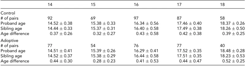
TABLE 1

Descriptive Statistics at Each Age

14 15 16 17 18

Control

# of pairs 92 69 97 87 58

Proband age 14.52±0.38 15.38±0.33 16.34±0.56 17.46±0.40 18.37±0.26 Sibling age 14.44±0.33 15.37±0.31 16.40±0.58 17.49±0.38 18.26±0.50 Age difference 0.37±0.26 0.32±0.27 0.43±0.58 0.42±0.38 0.39±0.25 Adoptive

# of pairs 77 54 76 77 40

Proband age 14.51±0.41 15.39±0.26 16.29±0.41 17.52±0.35 18.48±0.28 Sibling age 14.52±0.37 15.38±0.29 16.44±0.58 17.51±0.35 18.23±0.53 Age difference 0.44±0.30 0.28±0.23 0.41±0.53 0.44±0.47 0.52±0.25

and changes in legal rights (e.g., ability to legally purchase cigarettes) may underlie important environmental changes during this time.

Materials and Methods

Sample

Participants were from the Colorado Adoption Project (CAP), a longitudinal study following adoptive children, matched controls, and their families (Plomin & DeFries, 1983;1985) approximately yearly from infancy into adult-hood. Adoptive probands were ascertained through two Denver adoption agencies, while control probands were re-cruited from hospitals and matched to adoptive families based on sex of proband, number of children in the family, age and occupation of father, and father’s years of educa-tion. Enrollment in the CAP occurred between 1976 and 1983, and resulted in a final sample of 245 adoptive fam-ilies and 245 matched control famfam-ilies (Rhea et al.,2013). The most proximal younger sibling of the proband (if avail-able) was also recruited into the study as they reached the age of the proband at first assessment, so that sibling pair similarity could be compared across adoptive and control families. While proband assessments at any age (e.g., age 14 years) generally clustered within a given year, there was variation in the birth years of the siblings tested at a given age. Siblings were also assessed approximately annually, so that it was possible to compare measures taken when both the proband and the sibling were at a given age (e.g., 14 years). In contrast, cross-sectional studies compare sibling similarity within a given test year (e.g., proband at age 14 years, sibling at age 11 years) when influences on substance use may vary in both source and magnitude. (For further details of the CAP recruitment and assessment protocols, refer to Rhea et al.,2013.)Table 1 shows the number of control and adoptive sibling pairs tested at each age.

The CAP includes early and frequent interviews for sub-stance use, biannually from ages 12 to 18 years. Due to low prevalence of any substance use in early adolescence, we began analysis with the age 14 years assessment. We used data from probands and siblings who were tested at the same age (i.e., age at time of assessment of the sibling was within one year of the proband’s test age; seeTable 1). When

individuals had multiple assessments within a year (starting at age 15 years), we selected those assessments that would minimize the test age gap within sibling pairs. Although we used identical procedures for adoptive and control families, there was a trend (in three out of five waves) for the mean difference between the test age of a proband and his/her sib-ling to be greater in adoptive families compared to control families. These mean differences were small and generally not significant, with the exception of the age 18 assessment (control age difference,M=0.39,SD=0.25; adoptive age difference,M=0.52,SD=0.25;t(96)=2.53,p=.013). Though significant, this difference corresponds to a mean test age difference of approximately 50 days at the age 18 years assessment.

Measures

Substance use was assessed two different ways: use versus no use ever (use/no use), and the quantity/frequency of use in the past month. Wording of the measures varied slightly depending on the assessment wave in which the data was collected.

Use/No Use

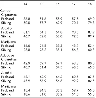
Use/no use was coded into dichotomous responses (0 = No, never; 1=Yes) for cigarettes, alcohol, and marijuana, based on the following questions: ‘Have you ever smoked cigarettes?’, ‘Have you ever had a drink of beer, wine, or liquor?’, and ‘Have you ever tried marijuana?’ respectively. At some assessment waves, quantity/frequency measures (described below) were collapsed into use/no use categories for alcohol and marijuana when not asked directly (e.g., quantity/frequency assessments includenoneandneverto identify non-users). Prevalence of use of cigarettes, alcohol, and marijuana at each age are shown inTable 2.

Quantity/Frequency of Substance Use

(4)

TABLE 2

Percent of Participants who Report Having Tried Substances at Least Once at Each Age

14 15 16 17 18

Control Cigarettes

Proband 36.8 51.6 55.9 57.5 69.0

Sibling 50.0 57.7 62.9 70.1 79.3

Alcohol

Proband 31.1 54.3 61.8 90.8 87.9

Sibling 46.7 62.8 68.0 92.0 89.7

Marijuana

Proband 16.0 24.5 33.3 43.7 53.4

Sibling 23.8 28.2 38.1 56.3 60.3

Adoptive Cigarettes

Proband 42.9 59.7 67.7 63.3 80.0

Sibling 40.7 51.4 54.5 68.8 65.0

Alcohol

Proband 48.1 62.9 64.2 80.5 87.5

Sibling 45.9 56.9 56.8 92.9 82.5

Marijuana

Proband 15.4 24.5 35.3 59.7 55.0

Sibling 18.6 31.0 35.2 54.5 55.0

Quantity/frequency of alcohol and marijuana use was also assessed ‘in the past month’ when direct assessments of that time frame were available; however, some assess-ments only asked about quantity/frequency of use ‘in the past 6 months’ or ‘in the past year’. In such cases, we re-coded responses into estimates of past month use in order to maintain consistency in the measure across time points. We assumed use was relatively stable across months and divided reported use by 6 or 12 to estimate use within a single month. Ultimately, ‘past month’ quantity/frequency responses (either directly assessed or estimated) were mea-sured on a 7-point scale (1= 0 times, 2=1–2 times, 3 =3–5 times, 4=6–9 times, 5=10–19 times, 6=20–39 times, 7=40 or more times). Notably,Table 3shows a gen-eral trend of increasing means and standard deviations for quantity/frequency across ages. This is consistent with the increasing prevalence of use across age inTable 2.

Data Transformation

For the analysis of dichotomous use/no use data, potential prevalence differences in substance use conditional on age, sex, and adoptive status were accommodated by estimat-ing thresholds separately for adoptive versus control siblestimat-ing pairs, and at each age. As seen inTable 2, there are strong age trends in the prevalence of use with greater use at older ages. There is also a trend (though less strong) for a higher prevalence of use among adoptive probands compared to non-adoptive probands. No significant sex differences in prevalence were observed across this age range.

Quantity/frequency data were transformed to minimize skewness. Within each subgroup (e.g., control probands, adoptive probands, control siblings, and adoptive siblings), we regressed quantity/frequency scores on sex and obtained

residuals. A constant of 5 was added to each standardized residual to remove negative values, and the residuals were then log transformed to minimize the positive skew. Fi-nally, log-transformed scores were standardized to facilitate interpretation of model parameter estimates. For descrip-tive purposes, raw scores are reported inTable 3. However, all biometrical analyses were conducted on standardized, transformed scores.

Analyses

Descriptive statistics and Pearson’s product moment correlations quantifying sibling resemblance for quan-tity/frequency of substance use in the past month were calculated using the Statistical Package for Social Sciences (IBM SPSS Statistics for Windows, Version 19.0). Genetic analyses were conducted using the software package Mx (Neale et al.,2006). Tetrachoric (sibling pair) correlations for substance use/no use were computed allowing for sepa-rate thresholds for probands and siblings, adoption status, and different thresholds for each assessment age.

Biometrical models accounted for the genetic covariance structure implicit in the adoption design. Briefly, the co-variance between control/biological siblings at a given time point can be parsed into additive genetic influences (a2_), and common environmental influence (c2). Within adop-tive sibling pairs, phenotypic similarity can only be due to common environmental influence in the absence of selec-tive placement. Non-shared environmental influences (e2) only contribute to the overall variance in a trait in a pop-ulation; the total variation in the population is assumed to be the sum of a2_{, c}2_{, and e}2_{. Due to sparse data issues, it was} not possible to fit multivariate models to the longitudinal ‘use’ data. Although we fit models to raw data, many of the 10×10 tetrachoric matrices (proband five waves×sibling five waves for each substance) were not positive definite. For both adoptive and sibling pairs, some cells of the matrices were empty or yielded correlations of±1.0. For this reason only univariate models for use/no use were conducted for the three substances at each of the five time points.

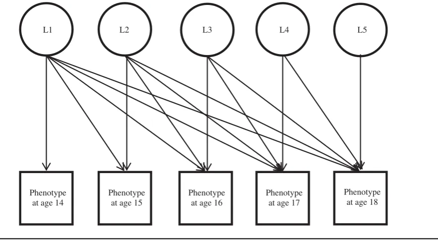
For multivariate models, a series of nested models were compared for goodness of fit using standard chi-square dif-ference tests (e.g., Neale & Cardon,1992). A basic Cholesky decomposition was used as a base model (see Figure 1; Neale & Cardon,1992). Since these models are a full de-composition of the variance-covariance matrix across all measurement occasions, they will necessarily provide a good fit to the data structure (i.e., the Cholesky decom-position is just-identified). Subsequent models were sidered to have good fit if the additional parameter con-straints did not result in a significant decrement in fit compared to the model fit of the corresponding Cholesky decomposition.

(5)

TABLE 3

Mean and Standard Deviation Quantity/Frequency of Use by at Each Age (Raw Scores)

14 15 16 17 18

Control

Cigarettes (n) 92 68 94 87 55

Proband 1.15±0.57 1.15±0.63 1.28±0.81 1.68±1.18 1.80±1.45 Sibling 1.12±0.39 1.29±0.96 1.35±0.92 1.63±1.05 1.75±1.42

Alcohol (n) 92 65 95 86 57

Proband 1.11±0.46 1.29±0.68 1.52±1.06 1.99±1.36 2.07±1.05 Sibling 1.17±0.57 1.49±0.90 1.58±0.91 2.15±1.38 2.40±1.22

Marijuana (n) 92 68 95 87 57

Proband 1.08±0.37 1.15±0.60 1.27±0.96 1.55±1.34 1.39±0.84 Sibling 1.14±0.66 1.29±0.99 1.32±1.02 1.84±1.68 1.63±1.36 Adoptive

Cigarettes (n) 75 53 76 76 40

Proband 1.24±0.75 1.36±0.83 1.50±1.08 1.92±1.41 2.10±1.44 Sibling 1.40±1.03 1.62±1.18 1.58±1.92 2.22±1.55 2.10±1.48

Alcohol (n) 74 53 76 74 40

Proband 1.28±0.80 1.40±0.79 1.64±1.13 2.19±1.50 2.30±1.22 Sibling 1.16±0.52 1.40±0.72 1.42±0.84 2.08±1.18 2.10±1.10

Marijuana (n) 75 52 75 76 39

Proband 1.09±0.52 1.21±0.98 1.38±1.05 1.57±1.46 1.62±1.46 Sibling 1.07±0.41 1.11±0.38 1.22±0.70 1.81±1.66 1.51±1.35

Note: quantity/frequency of use was measured on a 7-point scale (1=0 times, 2=1–2 times, 3=3–5 times, 4=6–9 times, 5=10–19 times, 6=20–39 times, 7=40 or more times) in the past month. Table entries include theNs, and mean±standard deviation.

Phenotype at age 14

Phenotype at age 15

Phenotype at age 16

Phenotype at age 17

Phenotype at age 18

L1 L2 L3 L4 L5

FIGURE 1

Basic cholesky decomposition model.

Note: Latent variables can further be decomposed into three separate latent variables reflecting the influences of additive genetics, shared environment, and non-shared environment.Figure 1shows the model for sibling-1 only; the model for sibling-2 is identical; correlations among the latent variables are fixed according to standard genetic theory and assumptions regarding shared and non-shared environmental influences.

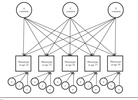
points, as well as age-specific influences (or residuals) that only explain variation at specific measurement occasions (seeFigure 2). These models allow the common genetic and environmental factors to influence the measured traits to different extents. Age-specific influences also may reflect important developmental changes across adolescence, such as novel influences coming ‘on-line’ at older ages.

(6)

A common

C common

E common

Phenotype at age 14

Phenotype at age 15

Phenotype at age 16

Phenotype at age 17

Phenotype at age 18

a c

e a

c e

a c

e a

c e a

c e

FIGURE 2.

Independent pathway model.

Note: Figure depicts an independent pathway model for sibling-1, for simplicity of presentation.

Results

Sibling Correlations for ‘Use/No Use’

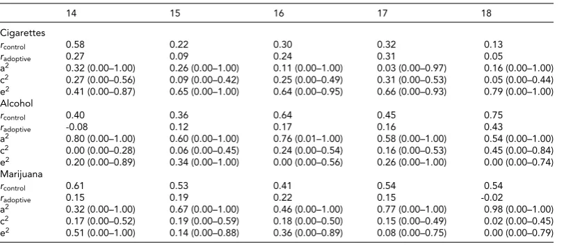
Table 4shows estimated tetrachoric sibling pair correlations for control pairs (who share both genetic and environmen-tal influences) and adoptive pairs (who share only environ-mental influences) at assessment ages 14 through 18 years. Across these ages, there was a consistent trend where control sibling pairs were more highly correlated for substance use than adoptive sibling pairs (seeTable 4).

Univariate Estimates for ‘Use/No Use’

Although confidence intervals are quite broad due to the di-chotomous nature of the data and the limited samples sizes at each age, the point estimates suggest substantial genetic influences (a2_{) on the liability to use alcohol and marijuana,} but only modest effects on cigarette use/no use. Shared en-vironmental (c2_{) estimates suggest small-to-moderate} in-fluence of the shared environment across substances and across ages. However, for alcohol use, there is some evi-dence for increasing shared environmental influences from age 14 to 18 years.

Sibling Correlations for ‘Quantity/Frequency’

Again, with a few exceptions (e.g., the youngest ages), con-trol sibling pairs were generally more highly correlated for

quantity/frequency of substance use than adoptive sibling pairs. Cross time point correlations were generally more strongly correlated with proximal time points compared to more distal ones.Table 5shows the full proband-sibling correlation matrix across the five time points. Adoptive proband-sibling correlations are shown above the diagonal and control proband-sibling correlations below.

Multivariate Biometrical Results

We reported raw scores for substance use quan-tity/frequency inTable 3to illuminate several trends (e.g., increasing means and variances across ages). However, sub-stance use variables were log-transformed and standardized prior to multivariate biometrical analysis so that path load-ings across ages could be interpreted on the same scale. Un-fortunately, sparse data issues, though not as severe as with our use/no use data, precluded fitting simplex models to the longitudinal data. It was necessary to utilize Cholesky de-composition and independent pathway models, which are more robust to sparse data issues.

(7)

TABLE 4

Sibling Correlationsa_{and Univariate Parameter Estimates for Use/No Use at Each Age}

14 15 16 17 18

Cigarettes

rcontrol 0.58 0.22 0.30 0.32 0.13 radoptive 0.27 0.09 0.24 0.31 0.05

a2 _{0.32 (0.00–1.00)} _{0.26 (0.00–1.00)} _{0.11 (0.00–1.00)} _{0.03 (0.00–0.97)} _{0.16 (0.00–1.00)} c2 _{0.27 (0.00–0.56)} _{0.09 (0.00–0.42)} _{0.25 (0.00–0.49)} _{0.31 (0.00–0.53)} _{0.05 (0.00–0.44)} e2 _{0.41 (0.00–0.87)} _{0.65 (0.00–1.00)} _{0.64 (0.00–0.95)} _{0.66 (0.00–0.93)} _{0.79 (0.00–1.00)} Alcohol

rcontrol 0.40 0.36 0.64 0.45 0.75 radoptive -0.08 0.12 0.17 0.16 0.43

a2 _{0.80 (0.00–1.00)} _{0.60 (0.00–1.00)} _{0.76 (0.01–1.00)} _{0.58 (0.00–1.00)} _{0.54 (0.00–1.00)} c2 _{0.00 (0.00–0.28)} _{0.06 (0.00–0.45)} _{0.24 (0.00–0.54)} _{0.16 (0.00–0.53)} _{0.45 (0.00–0.84)} e2 _{0.20 (0.00–0.89)} _{0.34 (0.00–1.00)} _{0.00 (0.00–0.56)} _{0.26 (0.00–1.00)} _{0.00 (0.00–0.74)} Marijuana

rcontrol 0.61 0.53 0.41 0.54 0.54 radoptive 0.15 0.19 0.22 0.15 -0.02

a2 _{0.32 (0.00–1.00)} _{0.67 (0.00–1.00)} _{0.46 (0.00–1.00)} _{0.77 (0.00–1.00)} _{0.98 (0.00–1.00)} c2 _{0.17 (0.00–0.52)} _{0.19 (0.00–0.59)} _{0.18 (0.00–0.50)} _{0.15 (0.00–0.49)} _{0.02 (0.00–0.45)} e2 _{0.51 (0.00–1.00)} _{0.14 (0.00–0.88)} _{0.36 (0.00–0.89)} _{0.08 (0.00–0.75)} _{0.00 (0.00–0.79)}

Note:a_{tetrachoric correlations.}

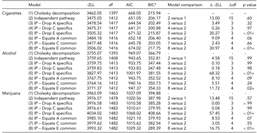
marijuana-assessed at five measurement occasions. Thus, we used the independent pathway as the base model for subsequent model comparisons to explore possible devel-opmental trends.

As a test of the significance of age-specific sources of variance, we compared a series of models where either the additive genetic (A), shared environmental (C), or non-shared environmental (E)specificswere dropped from the base independent pathway models (Models 3–5). Specifics were dropped independently (e.g., Model 3 dropped addi-tive genetic specifics while shared environmental and non-shared environmental specifics remained in the model). Across all substances, there was a significant decrement in fit only when dropping the age-specific non-shared envi-ronmental variance components (Model 5). There were no significant age-specific additive genetic or shared environ-mental influences. Although we had limited power, it can be seen fromTable 7 that the point estimates for specific A and C, with few exceptions, are small and quite often zero.

To test the stability of common influences, we also tested a series of models where the common additive genetic, shared environmental, or non-shared environmental path-ways were constrained to be equal (Models 6–8). Across all substances, the additive genetic and shared environmental influences could be constrained to be equal; indicating sub-stantial stability across adolescence. However, some caution in interpretation is warranted, given power issues. Non-shared environmental pathways across ages were the most variable and could not be constrained to be equal across age for all three substances.

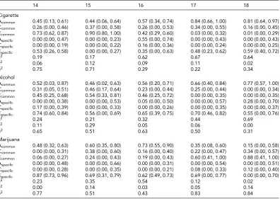
Standardized parameter estimates and confidence inter-vals for the base (full ACE) independent pathway models for each substance are shown inTable 7. The total proportion of variance explained by additive genetic (a2_{), shared} envi-ronmental (c2_{), and non-shared environmental (e}2_{) factors}

(i.e., common plus specific influences combined) are also reported.

Discussion

The current study utilized a longitudinal adoption design to examine the magnitude and developmental patterns of ge-netic and environmental influences on substance use from ages 14 to 18 years. Importantly, results from adoption stud-ies can be used to anchor estimates of environmental influ-ences that are indirectly assessed from twin studies, but directly estimated in sibling adoption designs.

(8)

TABLE 5

Correlations for Quantity/Frequency of Use in Past Month at Each Age

Proband Sibling

14 15 16 17 18 14 15 16 17 18

Cigarettes

Proband14 1.00 0.72 0.60 0.50 0.06 0.07 0.04 0.18 -0.16 0.06

15 0.92 1.00 0.42 0.28 0.03 0.08 0.15 -0.07 -0.06 -0.17

16 0.53 0.66 1.00 0.38 0.42 0.21 0.13 0.17 -0.18 0.08

17 0.27 0.25 0.67 1.00 0.67 0.21 0.26 0.16 0.06 0.19

18 0.06 -0.07 0.52 0.66 1.00 -0.01 0.19 0.23 -0.29 -0.01

Sibling 14 -0.06 -0.06 0.20 0.50 0.24 1.00 0.80 0.56 0.51 0.40

15 -0.05 -0.06 0.45 0.27 0.27 0.84 1.00 0.71 0.60 0.30

16 -0.05 -0.06 0.40 0.33 0.37 0.45 0.63 1.00 0.52 0.52

17 0.18 -0.01 0.43 0.41 0.45 0.39 0.40 0.60 1.00 0.66

18 0.11 -0.09 0.28 0.46 0.25 0.48 0.63 0.49 0.78 1.00

Alcohol

Proband14 1.00 0.57 0.53 0.31 0.27 0.26 -0.02 0.12 0.17 0.22

15 0.43 1.00 0.52 0.41 0.43 0.02 0.13 0.04 0.23 -0.27

16 0.41 0.68 1.00 0.41 0.45 0.14 0.11 -0.01 0.20 -0.18

17 0.36 0.18 0.55 1.00 0.50 -0.18 0.12 0.04 0.18 -0.22

18 0.29 0.30 0.43 0.71 1.00 -0.10 -0.10 -0.06 0.19 -0.10

Sibling 14 0.02 0.16 0.22 0.52 0.27 1.00 0.42 0.50 0.26 0.32

15 0.25 0.34 0.41 0.39 0.50 0.60 1.00 0.66 0.71 0.50

16 0.12 0.22 0.41 0.19 0.39 0.42 0.57 1.00 0.56 0.42

17 0.16 0.30 0.27 0.26 0.28 0.27 0.46 0.34 1.00 0.55

18 -0.12 0.00 0.24 0.24 0.39 0.08 0.37 0.49 0.39 1.00

Marijuana

Proband14 1.00 0.10 0.31 0.19 -0.09 -0.09 -0.13 -0.09 -0.01 -0.10

15 0.69 1.00 0.55 0.51 0.62 -0.06 0.20 0.15 -0.09 0.26

16 0.62 0.78 1.00 0.47 0.75 -0.12 0.09 -0.01 -0.14 0.07

17 0.35 0.35 0.25 1.00 0.65 0.27 -0.06 -0.04 -0.06 0.01

18 0.34 0.43 0.40 0.79 1.00 -0.01 0.54 0.24 -0.15 0.13

Sibling 14 0.08 -0.07 0.42 0.10 0.20 1.00 -0.07 0.40 -0.07 -0.10

15 0.54 0.32 0.27 0.21 0.33 0.18 1.00 0.19 0.19 0.52

16 0.33 0.32 0.19 0.33 0.40 0.24 0.69 1.00 0.28 0.23

17 0.38 0.36 0.17 0.27 0.41 0.19 0.45 0.45 1.00 0.76

18 -0.08 -0.09 -0.03 0.11 0.20 0.34 0.50 0.32 0.59 1.00

Note: Bold type indicates adoptive family correlations, normal typeface indicates control family correlations. Within-proband cor-relations are in top left quadrant, sibling-proband corcor-relations are in bottom left quadrant (control) and top right quadrant (adoptive), and within-sibling correlations are in bottom right quadrant.

TABLE 6

Model Comparisons of Biometrical Models for Five Ages With Standardized Variables

Model -2LL df AIC BICa _{Model comparison} _-2LL _df _{p value}

Cigarettes (1) Cholesky decomposition 3462.05 1397 668.05 215.94 – – – – (2) Independent pathway 3475.05 1412 651.05 206.17 2 versus 1 13.00 15 .60 (3) IP – Drop A specifics 3478.54 1417 644.54 202.49 3 versus 2 3.49 3 .32 (4) IP – Drop C specifics 3475.31 1417 641.31 200.88 4 versus 2 0.26 3 .97 (5) IP – Drop E specifics 3505.32 1417 671.32 215.87 5 versus 2 30.27 3 <.01∗ (6) IP – Equate A common 3484.18 1416 652.18 206.40 6 versus 2 9.09 4 .06 (7) IP – Equate C common 3477.48 1416 645.78 203.05 7 versus 2 2.43 4 .66 (8) IP – Equate E common 3506.02 1416 674.02 217.75 8 versus 2 30.97 4 <.01∗ Alcohol (1) Cholesky decomposition 3755.07 1393 969.07 366.79 - - -

-(2) Independent pathway 3759.65 1408 943.65 352.81 2 versus 1 4.58 15 .99 (3) IP – Drop A specifics 3759.75 1413 933.75 347.44 3 versus 2 0.10 3 .99 (4) IP – Drop C specifics 3759.83 1413 933.83 347.48 4 versus 2 0.18 3 .98 (5) IP – Drop E specifics 3827.97 1413 1001.97 381.55 5 versus 2 68.32 3 <.01∗ (6) IP – Equate A common 3767.75 1412 943.75 352.52 6 versus 2 8.10 4 .09 (7) IP – Equate C common 3764.16 1412 940.16 350.73 7 versus 2 5.51 4 .24 (8) IP – Equate E common 3771.37 1412 947.37 354.33 8 versus 2 11.72 4 .02∗ Marijuana (1) Cholesky decomposition 3963.09 1463 1037.09 394.88 - - -

-(2) Independent pathway 3976.57 1478 1020.56 387.98 2 versus 1 13.48 15 .57 (3) IP – Drop A specifics 3976.58 1483 1010.58 385.28 3 versus 2 0.00 3 >.99 (4) IP – Drop C specifics 3976.61 1483 1010.61 379.95 4 versus 2 0.04 3 .99 (5) IP – Drop E specifics 4034.02 1483 1068.02 408.66 5 versus 2 57.45 3 <.01∗ (6) IP – Equate A common 3985.10 1482 1021.10 379.93 6 versus 2 8.53 4 .07 (7) IP – Equate C common 3979.62 1482 1015.62 382.54 7 versus 2 3.05 4 .55 (8) IP – Equate E common 3993.32 1482 1029.32 289.39 8 versus 2 16.75 4 <.01∗

(9)

TABLE 7

Standardized Variance Estimates, Standardized Path Coefficients, 95% Confidence Intervals for Independent Pathway Results (Model 2)

14 15 16 17 18

Cigarette

Acommon 0.45 (0.13, 0.61) 0.44 (0.06, 0.64) 0.57 (0.34, 0.74) 0.84 (0.66, 1.00) 0.81 (0.64, 0.97) Ccommon 0.26 (0.00, 0.46) 0.37 (0.00, 0.58) 0.26 (0.00, 0.53) 0.34 (0.00, 0.55) 0.16 (0.00, 0.45) Ecommon 0.73 (0.62, 0.87) 0.90 (0.80, 1.00) 0.42 (0.29, 0.60) 0.03 (0.00, 0.32) 0.01 (0.00, 0.29) Aspecific 0.00 (0.00, 0.47) 0.00 (0.00, 0.23) 0.55 (0.00, 0.74) 0.00 (0.00, 0.43) 0.00 (0.00, 0.43) Cspecific 0.00 (0.00, 0.19) 0.00 (0.00, 0.22) 0.16 (0.00, 0.36) 0.00 (0.00, 0.24) 0.00 (0.00, 0.25) Especific 0.53 (0.26, 0.58) 0.00 (0.00, 0.27) 0.35 (0.00, 0.63) 0.48 (0.23, 0.62) 0.59 (0.40, 0.72)

a2 _0.19 _0.17 _0.62 _0.67 _0.64

c2 _0.06 _0.12 _0.09 _0.11 _0.02

e2 _0.75 _0.71 _0.29 _0.22 _0.34

Alcohol

a2 _0.24 _0.21 _0.32 _0.44 _0.69

c2 _0.11 _0.29 _0.05 _0.06 _0.00

e2 _0.65 _0.51 _0.63 _0.50 _0.31

Marijuana

a2 _0.23 _0.35 _0.54 _0.12 _0.02

c2 _0.00 _0.14 _0.03 _0.05 _0.14

e2 _0.77 _0.51 _0.43 _0.83 _0.84

Note: a2_{, c}2_{, and e}2_{reflect the total additive genetic, shared environmental, and non-shared environmental variance (e.g., common} and specific combined). Standardized variance estimates may not add up to 1.00 due to rounding.

adult years. In contrast, Koopmans et al. (1997) found sub-stantial early (age 12–14 years) shared environmental influ-ences for males only, while female alcohol use had strong early genetic influences. In contrast to Kendler et al. (2008), our study found that shared environmental influences on liability to use marijuana were modest across the range from age 14 to 18 years. Similarly, Baker et al. (2011) described a common factor model with substantial genetic effects on marijuana and illicit drug use/no use at age 13–14 years, with few additional innovative genetic affects emerging at ages 16–17 and 19–20 years.

Our adoptive and control sibling correlations for quan-tity/frequency of substance use generally suggest genetic influences, with only modest effects of the shared environ-ment, particularly at early ages when prevalence of use was lower. Additive genetic factors have also been shown to con-tribute substantially to substance use across development. A meta-analysis by Bergen et al. (2007) found an increase in the heritability for multiple phenotypes from adolescence into adulthood but no significant increases for two sub-stance use measures (i.e., nicotine initiation and alcohol consumption).

Although substance use is correlated across measure-ment occasions, it is possible that particular environmen-tal shifts (e.g., starting high school) or biological changes

(e.g., beginning puberty) may influence behavior at specific periods of adolescence. Thus, we fitted multivariate biomet-ric models to test whether use patterns across five ages had common influences or age-specific influences.

Overall, all age-specific genetic and shared environmen-tal influences could be dropped from cigarette, alcohol, and marijuana quantity/frequency of use models (e.g., Models 3–5 inTable 6). Age-specific, non-shared environmental in-fluences may reflect measurement error rather than unique environmental influences that could influence substance use at multiple waves.

(10)

(p=.24–.66). Common non-shared environmental path-ways were highly variable and could not be constrained for any substance. Given that few age-specific influences were detected, the total proportion of variance explained by addi-tive genetics and shared environment follow similar trends. There are several limitations to consider when interpret-ing these results. A potential confound of the CAP sam-ple was that there are more same-sex sibling pairs in the control families, while the adoptive families included more opposite-sex pairs. If same-sex sibling pairs are more simi-lar than opposite-sex pairs on substance use behaviors, the increased similarity of the control families (due to greater numbers of same-sex siblings) could bias our estimates of variance due to genetic effects upward. To test this, we ran a series of regression analyses to test the effect of adoption versus control status, same sex versus opposite sex status, and their interaction on sibling pair difference scores for quantity/frequency of use. Across five time points for each substance, same sex pairs were not significantly more sim-ilar than opposite sex pairs, nor were these effects different across adoptive and control families. For use/no use, we used logistic regression to test the same effects on pair con-cordance and discon-cordance. Across five time points for each substance, the test of the same sex/opposite sex effect was significant only once. However, the effect was in the oppo-site direction than expected. Oppooppo-site sex pairs were more similar for age 17 years alcohol use than same sex pairs, and this was more true for adoptive pairs than control pairs. Thus, there is no evidence in our data to suggest that the greater similarity of control siblings compared to adoptive siblings can be explained by the difference in same-sex ver-sus opposite-sex pairs.

Second, we did not have identical assessment questions throughout the length of the study. Our transformation from 6-month use or year use variables into past-month variables required some assumptions; namely, that average use over the past month was consistent with the given time span. For example, if a participant reported us-ing marijuana once a month on average over the past 6 months (or year), they would have been coded as using once during the past month, although they may have used more or less during different peak times over the year.

Finally, the numbers of adoptive and non-adoptive sib-ling pairs available at each age were relatively small in this study. This was primarily due to the requirement that both proband and sibling be tested within the same test age year-which was necessary for yearly assessment of the sibling pairs. This led to some sparse data issues that limited our approaches to data analysis (e.g., multivariate analysis of the use/no use was not possible; and multivariate analysis of the quantity/frequency data required use of methods that were robust to sparse data issues).

Despite these limitations, our study provides a unique contribution to the literature on genetic and environmental influences on substance use behavior. As the first

sibling-based longitudinal adoption study of substance use, our estimates provide a test of the role of environment on use of cigarettes, alcohol, and marijuana from adolescence into early adulthood. These estimates corroborate the point es-timates of cross-sectional twin studies and other prospec-tive designs. Importantly, the general trend of increasing genetic influences in late adolescence/early adulthood for quantity/frequency of alcohol use mirrors results reported from a recent parent–offspring longitudinal adoptive design (McGue et al.,2014). In conclusion, results of the present study indicate that individual differences in substance use from 14 to 18 years of age are largely due to common in-fluences. Moreover, although the sample of adopted and control sibling pairs was relatively small, our findings sug-gest that frequency/quantity of substance use during ado-lescence are due substantially to genetic influences, and that new genetic influences may emerge for cigarette and alcohol use in late adolescence.

Ethical Standards

The authors assert that all procedures contributing to this work comply with the ethical standards if the relevant na-tional and instituna-tional committees on human experimen-tation and with the Helsinki Declaration of 1975, as revised in 2008.

Acknowledgments

We greatly appreciate the participation of the CAP fam-ilies and the work of the Institute for Behavioral Genet-ics interview staff. This research was supported by grants HD010333, HD036773, & AG046938. Author Huibregtse was supported by T32 DA017637-11.

References

Baker, J. H., Maes, H. H., Larsson, H., Lichtenstien, P., & Kendler, K. S. (2011). Sex difference and developmental stability in genetic and environmental influences on psy-choactive substance consumption from early adolescence to young adulthood.Psychological Medicine, 9, 1907–1916. Bergen, S. E., Gardner, C. O., & Kendler, K. S. (2007). Age-related changes in the heritability of behavioral phenotypes over adolescence and young adulthood: A meta-analysis. Twin Research and Human Genetics, 10, 423–433.

Buchanan, J. P., McGue, M., Keyes, M., & Iacono, W. G. (2009). Are there shared environmental influences on adolescent behavior? Evidence from a study of adoptive siblings. Be-havior Genetics, 39, 532–540.

Distel, M. A., Vink, J. M., Bartels, M., Van Beijsterveldt, C. E. M., Neale, M. C., & Boomsma, D. I. (2011). Age mod-erates non-genetic influences on the initiation of cannabis use: A twin-sibling study in Dutch adolescents and young adults.Addiction,106, 1658–1666.

(11)

yses.Addiction, 94, 981–993.

Kendler, K. S., Schmitt, E., Aggen, S. H., & Prescott, C. A. (2008). Genetic and environmental influences on alcohol, caffeine, cannabis, and nicotine use from early adolescence to middle adulthood. Archives of General Psychiatry, 65, 674–682.

Koopmans, J. R., Lorenz, J. P., & Boomsma, D. I. (1997). Asso-ciation between alcohol use and smoking use in adolescent and young adult twins: A bivariate genetic analysis. Alco-holism: Clinical and Experimental Research, 21, 537–546. Lopez-Leon, M., & Raley, J. (2012). Developmental risks for

substance use in adolescence: Age as risk factor. In R. Rosner (Ed.),Clinical handbook of adolescent addiction(pp. 132– 138). Chichester, UK: Wiley-Blackwell.

Maes, H. H., Sullivan, P. F., Bulik, C. M., Neale, M. C., Prescott, C. A., Eaves, L. J., & Kendler, K. S. (2004). A twin study of genetic and environmental influences on tobacco initiation, regular tobacco use and nicotine dependence.Psychological Medicine, 34, 1251–1261.

Maes, H. H., Woodard, C. E., Murrelle, L., Meyer, J. M., Silberg, J. L., Hewitt, J. K., . . . Eaves, L. J. (1999). Tobacco, alcohol and drug use in eight- to sixteen-year-old twins: The Virginia twin study of adolescent behavioral development. Journal of Studies on Alcohol,60, 293–305.

McGue, M., Malone, S., Keyes, M., & Iacono, W. G. (2014). Parent-offspring similarity for drinking: A longitudinal adoption study.Behavior Genetics, 44, 620–628.

McGue, M., Sharma, A., & Benson, P. (1996). Parent and sibling influences of adolescent alcohol use and misuse: Evidence from a U.S. adoption cohort.Journal of Studies on Alcohol, 57, 8–18.

Neale, M., & Cardon, L. (1992).Methodology for genetic studies of twins and families. Dordrecht: Springer Science & Busi-ness Media.

tistical modeling. Richmond, VA: Department of Psychiatry. 7th Edition.

Pagan, J., Rose, R., Viken, R., & Pulkkinen, L. (2006). Genetic and environmental influences on stages of alcohol use across adolescence and into young adulthood.Behavior Genetics, 36, 483–497.

Plomin, R., & DeFries, J. C. (1983). The Colorado adoption project.Child Development, 54, 276–289.

Plomin, R., & DeFries, J. C. (1985). A parent-offspring adop-tion study of cognitive abilities in early childhood. Intelli-gence,9, 341–356.

Rhea, S. A., Bricker, J. B., Corley, R. P., DeFries, J. C., & Wadsworth, S. J. (2013). Design, utility, and history of the Colorado Adoption Project: Examples involv-ing adjustment interactions.Adoption Quarterly,16, 17– 39.

Rhee, S. H., Hewitt, J. K., Young, S. E., Corley, R. P., Crowley, T. J., & Stallings, M. C. (2003). Genetic and environmental influences on substance initiation, use, and problem use in adolescents. Archives of General Psychiatry, 60, 1256– 1264.

Rose, R. J., Dick, D. M., Viken, R. J., Pulkkine, L., & Kaprio, J. (2001). Drinking or abstaining at age 14? A genetic epi-demiological study.Alcoholism: Clinical and Experimental Research, 11, 1594–1604.

Verweij, K. J. H., Zietsch, B. P., Lynskey, M. T., Medland, S. E., Neale, M. C., Martin, N. G., . . . Vink, J. M. (2010). Ge-netic and environmental influences on cannabis use initia-tion and problematic use: A meta-analysis of twin studies. Addiction,105, 417–430.