000 0000
A frailty-model based approach to estimating the age-dependent penetrance
function of candidate genes using population-based case-control study designs:
An application to data on the BRCA1 gene
Lu Chen1, Li Hsu2,∗, and Kathleen Malone2
1Department of Preventive Medicine, University of Southern California, Los Angeles, CA,
and Children’s Oncology Group, Arcadia, CA, USA.
2Fred Hutchinson Cancer Research Center Division of Public Health Sciences Seattle, USA
*email:[email protected]
Summary:
The population-based case-control study design is perhaps one of, if not the most, commonly used
designs for investigating the genetic and environmental contributions to disease risk in epidemiologic
studies. Ages at onset and disease status of family members are routinely and systematically collected
from the participants in this design. Considering age at onset in relatives as an outcome, this paper
is focused on using the family history information to obtain the hazard function, i.e., age-dependent
penetrance function, of candidate genes from case-control studies. A frailty-model based approach
is proposed to accommodate the shared risk among family members that is not accounted for by
observed risk factors. This approach is further extended to accommodate missing genotypes in family
members and a two-phase case-control sampling design. Simulation results show that the proposed
method performs well in realistic settings. Finally, a population-based two-phase case-control breast
cancer study of the BRCA1 gene is used to illustrate the method.
Key words: Age-dependent penetrance function; BRCA1; Candidate gene; Case-control study
design; Nonparametric maximum likelihood; Semiparametric survival analysis.
1. Introduction
The population-based case-control study design is commonly employed in epidemiologic
studies of chronic disease etiology and recently has been used in studying genetic association
with disease risk. The odds ratios associated with mutations in these genes are estimated in
the same approach as that for environmental exposures by using the logistic regression model
as if the cases and controls were prospectively collected (Prentice and Pyke, 1979). When
disease prevalence is low, the odds ratio approximates the relative but not the absolute risk.
The absolute risk, unfortunately, is not estimable directly from case-control data because the
proportion of cases in the sample is fixed artificially by design. Whittemore (1995) proposed
the use of family data to estimate population-based baseline disease probability along with
odds ratios and correlation coefficients of disease status among family members under the
case-control study design. This approach requires factors of interest to be known for all
family members, an assumption which is not satisfied in a typical case-control study because
while family history of disease data are systematically collected for these cases and controls,
relatives’ exposure information is not. Fortunately this issue is less of a problem for studies
of candidate genes than environmental exposures as the carrier status for relatives can be
inferred probabilistically from the genotypic status of cases and controls by Mendel’s law.
This paper is thus focused on using family data gleaned through a case-control study design
to estimate the disease risk of candidate genes.
Age is an important risk factor for many chronic diseases and investigators typically collect
onset ages in relatives as part of disease family history information. This allows us to treat
onset age as a censored survival outcome and to take the advantage of recent methodologic
developments in multivariate survival analysis for estimating the cumulative risk, which is
also called the age-dependent penetrance function in the genetic epidemiologic literature.
population-based candidate gene studies in the context of volunteer-population-based studies. This study design goes
by several names including the kin-cohort design and the genotyped-proband design (Gail
et al., 1999). Methods of moments (Wacholder et al., 1998) and nonparametric maximum
likelihood (Chatterjee and Wacholder, 2001) methods have been developed for obtaining
hazard functions for individuals who do and do not carry high risk genotypes. However, these
methods tend to yield biased hazard function estimators for case-control studies because of
(i) the over-representation of cases due to the nature of the sampling and (ii) the residual
dependency among relatives even after accounting for candidate gene effects. Therefore,
methods that can both utilize relatives’ outcome and account for case-control sampling are
necessary for analyzing case-control data with family history information.
To circumvent the sampling and residual dependency issues, Chatterjee et al. (2006)
proposed to model the joint distribution of failure times of family members by a copula
model. In this approach, the Cox proportional hazards model (Cox, 1972) was used for the
marginal hazard function which represents population-averaged disease risks for carriers and
non-carriers. Such estimates are important particularly in terms of public health impact.
However, an individual is often more interested in the risk given his/her specific family
background. The latter naturally leads to a conditional hazard function formulation, in that
a frailty is assumed to represent the common unobserved risk for the family and it acts on
the hazard function in a multiplicative fashion.
The purpose of this paper is to present a newly developed frailty-model-based method
for estimating the hazard function from two-phase case-control data with family history
information. The baseline hazard function in the frailty model is left unspecified, allowing
for any arbitrary failure time distribution (age-dependent penetrance function). In Section
2, we first consider the situation where genotypes are observed for all family members and
more typical situation. We then examine the performance of the proposed methods by a
simulation study in Section 3. To demonstrate the potential insights that could be gleaned
from population-based studies with this method, we apply our approach to data on the
BRCA1 gene in Section 4. We conclude the paper with some final remarks.
2. Methods
2.1 Notation, Data structure, and Model Framework
Consider a two-phase case-control study. In the first phase a pool of cases and controls, here
termed as probands, are randomly sampled from the population and an array of risk factors
is collected from them. Stratified by certain aspects of variables collected at the first phase,
in the second phase a random subset of cases and controls from each stratum are selected for
collecting more detailed risk factor information, here, genotyping. The sampling fraction π
for a genotyped proband is therefore the fraction of individuals being randomly selected for
genotyping in the stratum to which the proband belongs. The sampling fraction is strictly
positive π > 0, i.e., all strata have representative samples, to ensure a consistent estimation
of odds ratios from two-phase data. When π = 1 for all strata, the two-phase sampling
design becomes the usual standard case-control design. The two-phase sampling scheme is
useful particularly when available resources constrain data collection for each individual.
By a careful choice of stratification variables and π, the two-phase design can improve the
efficiency of parameter estimates compared with a conventional case-control design with the
same number of subjects. This design has been used in many genetic epidemiologic studies
including the CARE study described further in Section 4 (Malone et al., 2006).
Below we introduce the notation and the model. Assume that there are n case-control
probands indexed by i = 1, . . . , n with sampling fraction π1, . . . , πn in a two-phase
from different families are non-overlapping. Specifically, in the ith family, let the proband
be indexed by subscript i0 and the ni relatives be indexed by subscript ij for j = 1, . . . , ni.
Furthermore let (Xij, δij, Zij) be the observational time, disease status, and a vector of
covariates for the jth individual in the ith family;δij is a disease indicator which is 1 if the
disease occurs at or before the censoring time and 0 otherwise, and Xij is the failure time if
δij = 1 and the censoring time if δij = 0. The total number of diseased in the ith family is
denoted by Δi =nj=0i δij. The observational time and disease status can also be equivalently
represented by the counting process notation. The right censored counting process Nij(t) is
defined as Nij(t) = I(Xij ≤ t, δij = 1), where I(·) is the indicator function. The at-risk
process Yij(t) is defined as Yij(t) =I(Xij ≥t).
We use a shared gamma frailty with the conditional proportional hazards model to describe
the dependent failure outcomes of family members. The unobserved frailty for the ith
family, represented byωi, induces dependence among family members on their failure times.
The family-specific frailty ωi is assumed to be iid gamma(1/θ, θ) distributed with density
θ−1/θΓ(1/θ)−1ωi1/θ−1exp(−ωi/θ) and mean 1. The parameter θ measures the strength of
dependence among failure times from family members, with a larger value of θ implying a
stronger dependence. The individual hazard function conditional on frailty and covariates is
given by
λij(t|Zij, ωi) = ωiλ0(t) exp(βZij), j = 0, . . . , ni, i= 1, . . . , n, (1)
where λ0(t) is the conditional baseline hazard function assumed common for all individuals
and β is a vector of regression coefficients. Conditional on the frailty and the covariates,
the censoring time is assumed to be independent of the failure time and non-informative of
the frailty. In addition, we assume that the frailty is independent of the observed covariates.
These assumptions are generally required by frailty models to allow for the distribution of
distribution and a parametric form for the effect of the risk factors, but leaves the form of
λ0(t) unspecified.
2.2 A likelihood function for the frailty model when all covariates are observed
To obtain valid estimates for {β,Λ0(t), θ}, we need to account for the case-control
retro-spective sampling. As relatives are sampled because of the proband’s disease outcomes and
sometimes ages at onset, a natural consideration for a likelihood-based approach in this
setting would be to let the joint likelihood of the relatives be conditional on the data from
the proband. In this likelihood, we do not make parametric assumptions on the form of Λ0(t).
To do this, we treat the jump size at each observed failure time as a parameter, following
the same idea as in the nonparametric maximum likelihood estimator (NPMLE) (Zeng and
Lin, 2007). However, direct maximization of our likelihood with respect to the jump sizes
is difficult because no closed form solution is available. We will show below that the frailty
formulation in conjunction with an EM-based algorithm provide a closed form maximum
likelihood solution to estimating Λ0(t).
In a shared frailty model, the latent frailty is typically viewed as missing data. A standard
approach for estimating parameters in the presence of missingness is to apply an EM
algorithm (Dempster et al., 1977). We will use a variation of this approach, the
expectation-conditional-maximization (ECM) algorithm (Meng and Rubin, 1993). The ECM algorithm
differs from the conventional EM algorithm in the maximization step, where the estimates for
multiple parameters are updated sequentially in an ECM algorithm rather than
simultane-ously as in the single M-step of an EM algorithm. It is particularly helpful when simultaneous
maximization with respect to all parameters is difficult.
To carry out an ECM algorithm, we first construct the complete likelihood assuming the
frailty were known. Under the assumptions given in Section 2.1, the complete likelihood
involving the parameters of interest {β,Λ0(t), θ}. The first term Li1 is the likelihood for
failure outcomes of the relatives conditional on the frailty and their covariates. It is the
product of contributions from each relative because of the conditional independence of the
relatives given the frailty and the covariates, and can be written as
Li1 =
ni
j=1
{ωiλ0(t) exp(βZij)}δijexp{−ωiΛ0(Xij) exp(βZij)}.
The second term Li2 is the likelihood of the frailty conditional on proband data. Since the
gamma distribution is a conjugate prior, the posterior distribution of ωi has a convenient
mathematical form
Li2 = ω
1/θ+δi0−1
i exp{−ωi/θ−ωiΛ0(Xi0) exp(βZi0)}
Γ(1/θ+δi0){1/θ+ Λ0(Xi0) exp(βZi0)}−1/θ−δi0.
Interestingly the likelihood function does not involveλ0(t) even when the proband is diseased,
but the involvement of Λ0(t) suggests that Λ0(t) may take jumps at the probands’ failure
times. We performed a simulation study assuming ω known for all probands who all had the
same age at onset t0 (for controls it would be age at last examination). We found that Λ0(t0)
and β were estimable from the data and the estimates appeared to be unbiased. In other
words, if Λ0(t0−) were known or estimated from the relatives’ data, the jump size at the
proband’s failure timest0would be estimable despiteLi2 does not involveλ0(t). However, the
two estimates, Λ0(t) and β, were highly collinear and the correlation coefficient was about
-0.90. For practical purposes it seems reasonable to allow Λ0(t) taking jumps only at the
relatives’ failure times but not the probands’, as there will be little information from the
probands for Λ0(t) taking jumps at probands’ failure times.
When the probands come from a two-phase sampling study design where each proband
is associated with a sampling fraction from the original stratum, the contribution of each
family needs to be adjusted accordingly. Research in the analysis of studies with two-phase
sampling design is very active, in the last two decades, see, e.g., Breslow and Chatterjee
weighted likelihood approach (Flanders and Greenland, 1991), where each selected proband
is weighed by the inverse selection probability 1/πi. Therefore the parameters are estimated
by maximizing
Lw = n
i=1
(Li1×Li2)
1 πi.
In the E-step, we estimate the expectation of the weighted log complete likelihood at
current parameter estimates. From the expression of log(Lw), it is easy to see that we
would only need to calculate the posterior expectations of ωi and lnωi, {1 + θΔi}/{1 +
θnj=0i Λ0(Xij) exp(βZij)}andφ(1/θ+Δi)−ln{1/θ+nj=0i Λ0(Xij) exp(βZij)}, respectively,
where φ(·) is the digamma function (Hougaard 2000, pp501).
In the CM-step, we update the parameter estimates sequentially between the finite
dimen-sional vector of (β, θ) and infinite dimensional vector of Λ0(t) by maximizing the expected
weighted log completed likelihood. Given the current estimateΛ0(t),βandθcan be updated
by maximizing the likelihood function via solving the score equations from taking the partial
derivative of the log-likelihood function with respect to (β, θ) using, for example, the
Newton-Raphson algorithm.
The maximization of the expected weighted log complete likelihood over Λ0(t) is more
complex. Fixing βand θat their current values, we obtain a closed-form expression for
Λ0(t) =
n i=1 ni j=1 t 0 1
S(u;β)dNij(u), (2)
whereS(u; β) is given byni=1nj=1i π1
iωiYij(u) exp(β
Zij)+n
i=1 π1i{ωi−ωi0}Yi0(u) exp(β Zi
0).
Here ωi0 equals (1 +θδi0)/{1 +θΛ0(Xi0) exp(βZi0)}, which is actually the expectation of
the frailty conditional on proband data. It is worth noting that the second term in S(u,β)
has an expectation of zero, suggesting that an alternative estimator for Λ0(t) could have the
same form as (2) with S(u,β) = in=1nj=1i π1
iωiYij(u) exp(β
Zij). This is the estimator that
the likelihood for the relatives’ data only, i.e.,ni=1Li1, with the addition of the weights. See
Web Appendix A for the derivation of (2).
The ECM algorithm described above is built upon formulation and maximization of a
weighted log likelihood. Since the baseline hazard function is estimated at the observed failure
times of the relatives, the dimension of the parameters involved inΛ0(t) increases with sample
size. The standard maximum likelihood theory for finite or fixed dimensional parameters does
not apply here. One may consider using the nonparametric information matrix weighted by
the inverse of sampling fractions to estimate the variance of the estimators following the
idea of Andersen et al. (1997) for cohort data under frailty models. The procedure involves
calculating and inverting a high dimensional matrix, which is quite complicated in both
analytical derivation and numerical implementation. As an alternative, we use bootstrap to
obtain the variance estimators. We would generate a fixed number, say, 100, of bootstrap
data sets, each consisted of the same number of case and control families resampled with
replacement from the original data set. Parameter estimates can then be obtained for each
bootstrap data set and the variance of the estimates over these bootstrap samples would be
the variance estimator of the parameter estimates from the original data set.
2.3 Extension for Relatives with Missing Genotypes
The ECM approach introduced in the previous section allows for handling the missing frailty
and now the missing genotypes in a unified fashion. Let g and Z be the genotype and the
observed covariates, andβandγ be the corresponding log-hazard ratios. Geneg is genotyped
for the probands, but not for the relatives and Z is assumed observed for each individual
including the probands and the relatives. For simplicity we assume g is a binary variable,
which is 1 if an individual carries one or two high risk alleles and 0 otherwise. This is
transmission models such as additive, recessive or an unrestricted general model which allows
for a separate hazard ratio for each different genotype.
Missing data now include the shared frailty and the genotypes for the relatives. To carry
out the ECM algorithm, we need to calculate the joint distribution for the shared frailty
and the genotypes for the relatives conditional on the observed data. This requires obtaining
the joint distribution of the genotypes for multiple relatives conditional on the genotype of
the proband. Unfortunately such joint distribution for genotype becomes very complex when
there are more than 2 relatives, as it depends on the joint familial relationship among all
family members. Incorporating such a complex joint distribution of the genotypes into the
joint distribution of frailty and missing genotypes given other observed data would make
the algebra rather complicated. Therefore, we consider a composite likelihood approach.
That is, instead of treating a family with multiple relatives and one proband as a unit, we
consider relative-proband pairs, viewing each relative-proband pair as a unit, and construct a
composite-likelihood by taking the product of the likelihoods from these units as if they were
independent even though there are multiple relative-proband pairs from the same family. In
this approach, the joint distribution of more than two family members does not need to be
explicitly worked out. This technique was first introduced in the longitudinal data setting
by Liang and Zeger (1986) under the name of generalized estimating equations and has also
been applied to family studies by, e.g., Chatterjee et al. (2006).
For the E-step of this ECM algorithm, we evaluate the expectation of ωi, lnωi, gij,
and ωiexp(βgij) conditional on the observed data from the proband-relative pairs. The
calculation of these expectations is in principle straightforward although it involves some
algebra. We denote those expectations by ˜E(ωi), ˜E(lnωi), ˜E(gij), and ˜E{ωiexp(βgij)}. See
For CM-step, we sequentially maximize the expression below with respect to β and γ: n i=1 1 πi ni j=1
δij{γZij +βE˜(gij)} −Λ0(Xi0) ˜E(ωi) exp(γZi0+βgi0)
−Λ0(Xij) exp(γZij) ˜E{ωiexp(βgij)}+ (1
θ +δi0) ln{
1
θ + Λ0(Xi0) exp(γ Z
i0+βgi0)} ,
and maximize the following expression with respect to θ:
n i=1 1 πi ni j=1 (1
θ +δi0) ln{
1
θ + Λ0(Xi0) exp(γ Z
i0+βgi0)}+ 1θ{E˜(lnωi)−E˜(ωi)} −ln{Γ(1
θ +δi0)} .
Note that the break down of a family with ni relatives into relative-proband pair can be
treated as if there were ni families and the proband is replicatedni times.
For updating Λ0(t), we obtain the following estimating equation:
Λ0(t) =
n i=1 1 πi n i j=1 t 0 1
S0(u;β, γ)dNij(u)
, (3)
whereS0(u;β, γ) =ni=1 π1
i
ni
j=1[Yij(u) exp(γZij) ˜E{ωiexp(βg ij)}+Yi0(u) exp(γZi0+βg i0)
{E˜(ωi)−ωi0}].
From the expressions it is clear that the ECM algorithm for data with missing genotypes in
the relatives follows closely to the ECM algorithm in Section 2.2, except that a generalized
likelihood rather than the full likelihood was used as the basis for the estimation. This
simplification was mainly to make computation manageable though at the price of a potential
efficiency loss and an invalid likelihood-based variance estimator. For the latter problem, we
again use re-sampling techniques as described in Section 2.2 to obtain variance estimators
for the parameter estimates.
2.4 Inclusion of Proband Data
The likelihood function of the proband dataP(Zi0, gi0|Xi0, δi0) is a retrospective likelihood for
the usual case-control data. If cases and controls are matched on age, the likelihood function
can be replaced by the conditional likelihood for estimation under the frailty model by adding
(Hsu et al., 2004). This approach, however, does not work for the two-phase design, where
cases and controls are each sampled based on their own stratum and the matched case-control
mechanism is not preserved. An alternative approach is to rewrite
P(Zi0, gi0|Xi0, δi0) = P(Xi0, δi0|Zi0, gi0)f(Zi0)f(gi0)
z∗
g∗P(Xi0, δi0|z∗, g∗)f(g∗)f(z∗)dz∗,
assuming the independence of Z and g in the population. The distribution f(Z) and the
allele frequency in f(g) need to be estimated from the data. The proband data alone do
not allow us to uniquely identify these population parameters and {β, γ,Λ0(t)}. However, in
conjunction with the relatives’ data, they are identifiable, as {β, γ,Λ0(t)} can be estimated
from the relatives. Since f(Z) is not of main interest, we propose to take an additional
condition given Zi0, that is, P(gi0|Xi0, δi0, Zi0). Under the two-phase sampling design, the
inverse-weighted log-likelihood function of the probands is given by
log(L) =
n
i=1
1
πilog
{1 +θΛ0(Xi0) exp(βgi0+γZi0)}−1/θ−δi0exp(βgi0δi0)f(gi0)
g∗{1 +θΛ0(Xi0) exp(βg∗+γZi0)}−1/θ−δi0exp(βg∗δi0)f(g∗),
Although the expression involves both θand Λ0(t), intuitively the proband likelihood cannot
provide direct information on them. We therefore use the proband likelihood log(L) only for
estimating β along with the relatives’ data and q. Note that in the absence of covariates
Zi0 and under the conventional case-control design, this likelihood function was proposed
by Chatterjee et al. (2006) for estimating allele frequency q, an important quantity that
investigators often are interested in estimating.
3. Simulation Studies
We performed a simulation study to evaluate the performance of the proposed method
under several realistic settings. In these simulations, we generated a candidate gene g and
a continuous risk factor Z for each individual, where g followed Mendelian transmission
with an autosomal dominant model and Z followed a N(0,1). We also generated a
a Weibull distribution with p = 4.6 and λ = 0.01. The failure time for each individual was
then generated according to the frailty model (1). Each family consisted of the proband, the
mother, and a sister. The censoring distribution wasN(60,15), yielding censoring percentage
about 80% - 85%.
We considered four different sampling scenarios for the simulation: a) no stratified sampling
of cases and controls; b) stratified sampling of cases only but not controls; c) stratified
sampling of controls only but not cases; and d) stratified sampling of both cases and controls.
For each of these scenarios, we started by randomly selecting a pool of 1800 case families and
a pool of 1800 control families from the population as the first phase sampling. The second
phase sampling of the families varies for the four scenarios. For scenario a, we randomly
chose 200 case families and 200 control families from each pool. For scenario b, we randomly
selected 200 control families and performed a stratified sampling of 200 case families based
on the number of diseased relatives that they had. If both the mother and the sister were
diseased, the proband was always selected for genotyping. Among the families with only
one diseased relative, we randomly selected 100 probands for genotyping. We then randomly
sampled from the remaining families in which neither of the relatives was diseased to reach
a total number of 200 case families. We employed a similar sampling strategy for selecting
control probands in scenario c and selecting case and control probands separately in scenario
d. The selection fraction is one, about one in three, and one in six to seven for families with
two, one, and no diseased relatives, respectively.
We considered two situations for the candidate gene effect: 1) rare allele (q = 0.05) but
relatively high penetrance (β = log(5) = 1.609) (Table 1), and 2) common allele (q = 0.2)
with relatively low hazard ratio (β = log(2) = 0.693) (Table 2). There were about 46–60
carriers among 200 cases and 15–19 carriers in 200 controls under the rare allele with high
controls under the common allele with moderate penetrance model. The number of carriers
generated under the rare allele high penetrance model is comparable to that in the BRCA1
data set that we will analyze in Section 4. In addition, θ takes two values: 0.5 for moderate
dependence and 1.5 for strong dependence. For each parameter setting, a total of 500 data
sets were simulated to assess the performance of the proposed method.
[Table 1 about here.]
[Table 2 about here.]
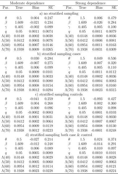
The biases appear to be small in all simulation situations. There is about 15-30% reduction
in the standard errors (SEs) of θand Λ0(t) when both cases and controls are sampled by
stratification compared to the other three sampling schemes. However, there is no efficiency
gain in βfor the genetic effect. If only cases or controls but not both are sampled based on
stratification, the SEs of β tend to be inflated compared to the sampling scheme without
any stratification. This loss of efficiency may be due to an additional variation induced by
the weights and/or the fact that a positive family history in our simulation setup is caused
not only by or the risk factors under study but also by the shared frailty. It seems that
stratifying based on positive family history with an intention of increasing the frequency of
high risk allele carriers may not necessarily translate into an efficiency gain forβfor candidate
genes. In these simulation settings, the inclusion of proband likelihood in the estimation of
β greatly increases the efficiency compared with the estimator without including proband
likelihood for β, the extent of which depends on the specific sampling schemes used in
the simulations (results not shown). This implies that the proband likelihood can provide
substantial information on β once other parameters are identified. Such an efficiency gain
was also observed in simulation studies in Chatterjee et al. (2006).
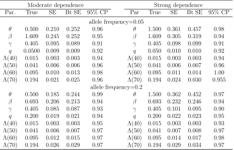
We used the bootstrap method to estimate the se of the ECM estimators. Here we present
is also the most comprehensive design. Table 3 shows empirical SE, bootstrap-based SE, and
bootstrap-based coverage probabilities (CP)of 95% confidence intervals for 200 simulated
data sets with 100 bootstrap samples from each simulated data set. Compared with the SDs
of parameter estimates over simulated data sets, the bootstrap-based SEs appear working
well for {β, γ} and q, but may over-estimate the SEs of θand Λ0(t). The CPs appear to
maintain 95% nominal level forβandq, but tend to be higher than nominal level forθand the
later time points of Λ0(t) and lower for γ. The under- or over- estimation of 95% coverage
probabilities are, to some extent, due to the small sample size. For θ, the overestimation
could also be due to the fact that our bootstrap sampling unit is by family. The dependence
parameter estimates are influenced by the number of families with more than one affected
relatives and the number for such families is usually small. So when one or a few such families
are in (or out of) the bootstrap samples, the estimates may be affected greatly.
[Table 3 about here.]
4. Application to a Breast Cancer Dataset
As an illustration, we applied the proposed methods to a breast cancer dataset to estimate
the hazard functions of developing breast cancer (BC) for BRCA genetic mutations. This
population-based case-control study was conducted within the National Institute of Child
Health and Human Development’s Women’s Contraceptive and Reproductive Experiences
(CARE) study (Marchbanks et al., 2002). Due to funding constraints, the study could only
collect blood from approximately 33% of the interviewed women and thus a second phase
sampling design was developed, where women were stratified sampled according to their
case-control status, study site, race, family history, and age. Within each stratum, a sampling
strata. A study of the BRCA1/2 genes was conducted to evaluate their contribution to breast
cancer risk (Malone et al., 2006).
For illustrative purpose, in this analysis we focus on only the BRCA1 gene and included
only White probands and their blood-related first degree relatives. BRCA2 carriers were
considered as non-carriers of BRCA1 mutations. The first degree relatives were restricted to
those age 18 or older and had known breast cancer status at the time of study. Among the
1603 White probands with known BRCA1 mutation status, 1144 (71%) are cases. There are
42 (3.8%) BRCA1 mutation carriers in cases and only 1 in controls. A total of 4568 first
degree relatives were included, and among them 634 (13.9%) had developed breast cancer.
We applied the method proposed in section 2.3 and included the likelihood of the proband
data in Section 2.4 for estimating the allele frequency. In this analysis we did not include
the proband likelihood in estimating relative risk because we observed a collinearity problem
between estimating β and allele frequency in the proband data. The collinearity is likely
due to the rare mutational frequency of the BRCA1 gene. Such rare allele frequency, on the
other hand, makes the estimation of β using relatives quite insensitive to changes in q, as
the carrier probability of a relative given the proband’s carrier status changes little with the
allele frequency when the frequency is low.
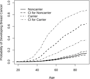
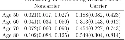
Figure 1 shows the estimated population cumulative cancer-free probabilities for BRCA1
mutation carriers and noncarriers and point-wise bootstrap confidence intervals. We present
here the marginalized probabilities integrating over the frailty distribution mainly for the
comparison of our result with those that have been published on other datasets (Table 4).
Bootstrap confidence intervals were obtained based on 200 bootstrap samples. Mutation
carriers had an estimated 45.4% or 54.9% chance of developing BC by age 70 or 80, in
comparison to noncarriers who had an estimated chance of 7.2% or 10.2% at the same
estimates reviewed by e.g. Chen and Parmigiani (2007). The estimates (β, theta, q) are 2.354
(95%CI: 1.374–3.534), 0.948 (95%CI: 0.505–1.444), and 0.181% (95%CI: 0.080%–0.401%),
respectively. The high valuetheta suggests there remains substantial residual dependency of
ages at onset among family members, which Begg et al. (2008) observed as well. It is also
worth noting that even though we assume β constant in the frailty model (1), the resulting
population averaged hazard ratio decreases over the age and they are 8.822, 7.677, 6.371,
and 5.479 at age 50, 60, 70, and 80 years old, respectively.
[Table 4 about here.]
[Figure 1 about here.]
An advantage of the frailty model approach is to provide a woman with an individualized
risk estimate. For example, a 40 year old woman who had a mother with BC diagnosed at age
38 and carried a BRCA1 mutation would have a 86.4% cumulative probability of developing
BC by age 80. The estimated frailty value in this case is 1.77. If she were not a mutation
carrier, with all other information the same her probability would be 18.7% with ω = 1.93.
Note that ω is slighted lower if the woman is a carrier than if she is a non-carrier, because
the BRCA1 mutation partly explains the aggregation of BC in a family. On the other hand,
if the same age woman did not carry a BRCA1 mutation and her mother were still disease
free at age 65, she would have only 9.6% chance of developing BC before age 80 (ω = 0.94).
As a bench mark, the average risk for a carrier and a non-carrier woman to develop breast
cancer regardless of family history is 54.9% and 10.2%, respectively.
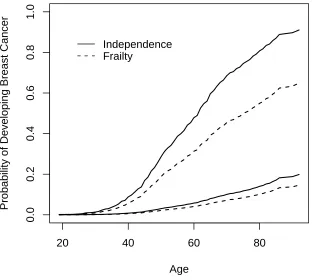
We also estimated the penetrance function assuming that the breast cancer risk for family
members is independent given BRCA1 genotype, in other words, BRCA1 genotypes among
family members explain completely the dependence of ages at onset among family members
the residual dependence among family members over-estimated the population breast cancer
risk for both carriers and noncarriers considerably (Figure 2).
[Figure 2 about here.]
5. Final Remarks
In this paper we developed a weighted likelihood approach to estimating regression
coeffi-cients, nonparametric baseline hazard function, and dependence parameter under a shared
frailty model from two-phase case-control data with family history information. While the
work is focused on the estimation of penetrance function for the BRCA1 gene, the method
is generalizable to other candidate genes. The family history information, which is typically
collected in epidemiologic studies, if of sufficiently high quality, can provide population
estimates that are not available from using case-control data alone. Moreover, the residual
dependency estimates can shed light on whether one or more candidate genes or other shared
environmental risk factors may contribute to diseases. Finally, the proposed likelihood, which
conditions on the probands’ survival time and allows for residual dependency via a frailty, is
robust against ascertainment biases that are often major issues in studies of gene penetrance.
Frailty models are useful especially when the goal is to make inference about individual
families, e.g., in the situation of genetic counseling. As genetic data are increasingly available,
public interests in genetic counseling are more intense than ever. It is thus critical to
provide an accurate estimate of carrier probability and individualized disease probability
for a counselee. Frailty model-based approaches that incorporate both the measured risk
factors and those that are unknown or unmeasured by a shared frailty are appealing in this
situation. One caveat, however, is that the estimate of individual risk depends on the frailty
distribution and a misspecification could bias the estimate even though the estimate for the
While nonparametric modeling puts no constraint in baseline hazard function, fitting
may become unstable especially when the gene is rare and disease incidence low. Weakly
parametric modeling, e.g., a three-parameter Weibull model proposed by Gail et al. (1999)
may be useful in regularizing the potentially high-dimensional baseline hazard function. In
principle the proposed approach should apply with much reduced computation. It would be
useful to provide this as an alternative to the nonparametric modeling.
Supplementary Materials
Web Appendices referenced in Sections 2.2 and 2.3 are available under the Paper Information
link at the Biometrics websitehttp://www.tibs.org/biometrics.
Acknowledgments
The authors thank all of the CARE Study Investigators and Staff for their leadership in
designing and conducting the CARE Study. The authors would also like to thank Dr. Nilanjan
Chatterjee from the National Cancer Institute for many helpful discussions during the course
of the methodologic development, and to the Associate Editor and the two anonymous
referees who have made many constructive comments, which have improved the manuscript
and stimulated future work.
This work is in part supported by the grants from the National Cancer Institute (AG14358,
CA53996)and the National Institute of Child Health and Human Development, with
addi-tional support from the Naaddi-tional Cancer Institute, through contracts with Emory University
(N01 HD 3-3168), Fred Hutchinson Cancer Research Center (N01 HD 2- 3166), Karmanos
Cancer Institute at Wayne State University (N01 HD 3-3174), University of Pennsylvania
(N01 HD 3-3176), University of Southern California (N01 HD 3-3175), and through an
References
Andersen, P. K., Klein, J. P., Knudsen, K.M., and Tabanera y Palacios, R. al. (1997).
Esti-mation of variance in Cox’s regression model with shared Gamma frailties. Biometrics
53, 1475–1484.
Begg, C. B., Haile, R. W., Borg, A., Malone, K. E., Concannon, P., Thomas, D.C., Langholz,
B., Bernstein, L., Olsen, J. H., Lynch, C. F., Anton-Culver, H., Capanu, M., Liang, X.,
Hummer, A. J., Sima, C., and Bernstein, J. L. (2008). Variation of breast cancer risk
among BRCA1/2 carriers. Journal of the American Medical Association 299, 194–201.
Breslow N.E. and Chatterjee N. (1999). Design and analysis of two-phase studies with binary
outcomes applied to Wilms tumor prognosis. Applied Statistics48, 457-468.
Chatterjee, N., and Wacholder, S. (2001). A marginal likelihood approach for estimating
penetrance from kin-cohort designs. Biometrics 57, 245–252.
Chatterjee, N., Zeymep, K., Shih, J.H., and Gail, M. H. (2006). Case-control and
case-only designs with genotype and family history data: estimating relative-risk, familial
aggregation and absolute risk. Biometrics 62, 36–48.
Chen, S. and Parmigiani, G. (2007). Meta-analysis of BRCA1 and BRCA2 penetrance.
Journal of Clinical Oncology 25, 1329–1333.
Cox, D. R. (1972). Regression models and life tables (with discussion). Journal of the Royal
Statistical Society B 34, 187–220.
Dempster, A. P., Laird, N. M., and Rubin, D. R. (1977). Maximum likelihood estimation from
incomplete data via the EM algorithm (with discussion).Journal of the Royal Statistical
Society B 39, 1–38.
Flanders, W. D., and Greenland S. (1991). Analytical methods for two-stage case-control
studies and other stratified designs. Statistics in Medicine 10, 739–747.
the penetrance of an identified autosomal dominant mutation: cohort, case-control, and
genotyped-proband designs. Genetic Epidemiology 16, 15–39.
Hougaard, P. (2000). Analysis of multivariate survival data. Springer-Verlag, New York.
Hsu, L., Chen, L., Gorfine, M., and Malone, K. E. (2004). Semiparametric estimation of
marginal hazard function from the case-control family studies. Biometrics 60, 936–944.
Hsu, L., Gorfine, M. and Malone, K. E. (2007). Effect of Frailty Distribution
Misspecifica-tion on Marginal Regression Estimates and Hazard FuncMisspecifica-tions in Multivariate Survival
Analysis. Statistics in Medicine 26, 4657–4678.
Liang, K. Y. and Zeger, S. L. (1986). Longitudinal analysis using generalized linear models.
Biometrika 73, 13–22.
Marchbanks, P. A., Mcdonald, J. A., Wilson, H. G., Burnett, N. M., Daling, J. R., Bernstein,
L., Malone, K. E., Strom, B. L., Norman, S. A., Weiss, L. K., Liff, J. M., Wingo, P.
A., Burkman, R. T., Folger, S. G., Berlin, J. A., Deapen, D. M., Ursin, G., Coates,
R. J., Simon, M. S., Press, M. F., and Spirtas, R. (2002). The NICHD women’s
contraceptive and reproductive experiences study: methods and operational results.
Annals of Epidemiology 26, 213–221.
Malone, K. E., Daling, J. R., Doody, D. R., Hsu, L., Bernstein, L., Coates, R. J., Marchbanks,
P. A., Simon, M. S., McDonald, J. A., Norman, S. A., Strom, B. L., Burkman, R. T.,
Ursin, G., Deapen, D., Weiss, L. K., Folger, S., Madeoy, J. J., Friedrichsen, D. M.,
Suter, N. M., Humphrey, M. C., Spirtas, R. and Ostrander, E. A. (2006). Prevalence and
predictors of BRCA1 and BRCA2 mutations in a population-based study of breast cancer
in white and black American women aged 35–64 years.Cancer Research 66, 8297–8308.
Meng, X. L. and Rubin, D. B. (1993). Maximum likelihood estimation via the ECM
algorithm: A general framework. Biometrika 80, 267–278.
Prentice, R. L. and Pyke, R.(1979). Logistic Disease Incidence Models and Case-Control
Studies. Biometrika 66(3), 403–411.
M. (1998). The kin-cohort study for estimating penetrance. American Journal of
Epi-demiology 148, 623–630.
Whittemore, A. S. (1995). Logistic regression of family data from case-control studies.
Biometrika textbf82, 57–67.
Zeng, D. and Lin, D. Y. (2007). Maximum likelihood estimation in semiparametric regression
20 40 60 80
0.0
0.2
0.4
0.6
0.8
1.0
Age
Probability of Developing Breast Cancer
Noncarrier CI for Noncarrier Carrier
CI for Carrier
20 40 60 80
0.0
0.2
0.4
0.6
0.8
1.0
Age
Probability of Developing Breast Cancer
Independence Frailty
Table 1
Biases and empirical standard errors (SEs) for the ECM approach for regression coefficients, dependence parameter and cumulative baseline hazard function at selected ages for a rare (q= 0.05) but high risk (β= log 5) gene. The data consist of (stratified) cases and controls and their mothers and sisters. The genotypes are missing by design in
the relatives.
Moderate dependence Strong dependence
Par. True Bias SE Par. True Bias SE
a) no stratified sampling
θ 0.5 0.004 0.247 θ 1.5 0.006 0.479
β 1.609 -0.021 0.234 β 1.609 -0.026 0.284
γ 0.405 -0.002 0.099 γ 0.405 0.005 0.100
q 0.05 0.0011 0.0074 q 0.05 0.0011 0.0079 Λ(40) 0.0148 0.0002 0.0038 Λ(40) 0.0148 0.0000 0.0036 Λ(50) 0.0412 0.0003 0.0076 Λ(50) 0.0412 0.0006 0.0081 Λ(60) 0.0954 0.0007 0.0146 Λ(60) 0.0954 0.0011 0.0163 Λ(70) 0.1938 0.0009 0.0265 Λ(70) 0.1938 0.0031 0.0309
b) stratified sampling cases
θ 0.5 0.030 0.284 θ 1.5 0.049 0.536
β 1.609 -0.007 0.275 β 1.609 0.007 0.320
γ 0.405 0.006 0.099 γ 0.405 0.005 0.110
q 0.05 0.0009 0.0101 q 0.05 0.0011 0.0112 Λ(40) 0.0148 0.0000 0.0033 Λ(40) 0.0148 0.0002 0.0036 Λ(50) 0.0412 0.0003 0.0080 Λ(50) 0.0412 0.0004 0.0083 Λ(60) 0.0954 0.0008 0.0154 Λ(60) 0.0954 0.0010 0.0160 Λ(70) 0.1938 0.0012 0.0294 Λ(70) 0.1938 0.0023 0.0315
c) stratified sampling controls
θ 0.5 -0.041 0.259 θ 1.5 -0.093 0.427
β 1.609 0.004 0.268 β 1.609 0.002 0.360
γ 0.405 0.000 0.096 γ 0.405 0.002 0.098
q 0.05 -0.0002 0.0083 q 0.05 0.0001 0.0103 Λ(40) 0.0148 0.0001 0.0031 Λ(40) 0.0148 0.0002 0.0030 Λ(50) 0.0412 0.0002 0.0064 Λ(50) 0.0412 0.0007 0.0067 Λ(60) 0.0954 0.0009 0.0119 Λ(60) 0.0954 0.0008 0.0130 Λ(70) 0.1938 0.0012 0.0223 Λ(70) 0.1938 -0.0001 0.0248
d) stratified sampling both case & control
θ 0.5 -0.027 0.214 θ 1.5 0.024 0.374
β 1.609 -0.012 0.248 β 1.609 -0.014 0.291
γ 0.405 0.006 0.089 γ 0.405 0.010 0.097
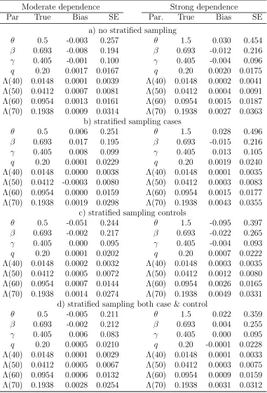
Table 2
Biases and empirical standard errors (SEs) for the ECM approach for regression coefficients, dependence parameter and cumulative baseline hazard function at selected ages for a common (q= 0.2) and low risk (β= log 2) gene. The data consist of (stratified) cases and controls and their mothers and sisters. The genotypes are missing by design in
the relatives.
Moderate dependence Strong dependence
Par True Bias SE Par. True Bias SE
a) no stratified sampling
θ 0.5 -0.003 0.257 θ 1.5 0.030 0.454
β 0.693 -0.008 0.194 β 0.693 -0.012 0.216
γ 0.405 -0.001 0.100 γ 0.405 -0.004 0.096
q 0.20 0.0017 0.0167 q 0.20 0.0020 0.0175 Λ(40) 0.0148 0.0001 0.0039 Λ(40) 0.0148 0.0002 0.0041 Λ(50) 0.0412 0.0007 0.0081 Λ(50) 0.0412 0.0004 0.0091 Λ(60) 0.0954 0.0013 0.0161 Λ(60) 0.0954 0.0015 0.0187 Λ(70) 0.1938 0.0009 0.0314 Λ(70) 0.1938 0.0027 0.0363
b) stratified sampling cases
θ 0.5 0.006 0.251 θ 1.5 0.028 0.496
β 0.693 0.017 0.195 β 0.693 -0.015 0.216
γ 0.405 0.008 0.099 γ 0.405 0.013 0.105
q 0.20 0.0001 0.0229 q 0.20 0.0019 0.0240 Λ(40) 0.0148 0.0000 0.0038 Λ(40) 0.0148 0.0001 0.0035 Λ(50) 0.0412 -0.0003 0.0080 Λ(50) 0.0412 0.0003 0.0083 Λ(60) 0.0954 0.0000 0.0159 Λ(60) 0.0954 0.0015 0.0177 Λ(70) 0.1938 0.0019 0.0298 Λ(70) 0.1938 0.0043 0.0355
c) stratified sampling controls
θ 0.5 -0.051 0.244 θ 1.5 -0.095 0.397
β 0.693 -0.002 0.217 β 0.693 -0.022 0.265
γ 0.405 0.000 0.095 γ 0.405 -0.004 0.093
q 0.20 0.0001 0.0202 q 0.20 0.0007 0.0222 Λ(40) 0.0148 0.0002 0.0032 Λ(40) 0.0148 0.0003 0.0035 Λ(50) 0.0412 0.0005 0.0072 Λ(50) 0.0412 0.0012 0.0080 Λ(60) 0.0954 0.0007 0.0144 Λ(60) 0.0954 0.0026 0.0165 Λ(70) 0.1938 0.0014 0.0274 Λ(70) 0.1938 0.0049 0.0331
d) stratified sampling both case & control
θ 0.5 -0.005 0.211 θ 1.5 0.022 0.359
β 0.693 -0.002 0.212 β 0.693 0.004 0.255
γ 0.405 0.006 0.083 γ 0.405 0.000 0.095
Table 3
Summary statistics of empirical standard errors (SE), bootstrap SEs (Bt SE), coverage probabilities of 95% bootstrap confidence intervals (95% CP) when both cases and controls are sampled according to the family history.
Moderate dependence Strong dependence
Par. True SE Bt SE 95% CP Par True SE Bt SE 95% CP
allele frequency=0.05
θ 0.500 0.210 0.252 0.96 θ 1.500 0.361 0.457 0.98
β 1.609 0.245 0.252 0.95 β 1.609 0.305 0.319 0.94
γ 0.405 0.095 0.089 0.91 γ 0.405 0.098 0.099 0.91
q 0.0500 0.009 0.009 0.92 q 0.050 0.010 0.010 0.92 Λ(40) 0.015 0.003 0.003 0.94 Λ(40) 0.015 0.003 0.003 0.94 Λ(50) 0.041 0.006 0.006 0.96 Λ(50) 0.041 0.006 0.007 0.96 Λ(60) 0.095 0.010 0.013 0.98 Λ(60) 0.095 0.011 0.014 1.00 Λ(70) 0.194 0.021 0.025 0.96 Λ(70) 0.194 0.024 0.030 0.955
allele frequency=0.2
θ 0.500 0.185 0.244 0.99 θ 1.500 0.362 0.452 0.97
β 0.693 0.206 0.213 0.94 β 0.693 0.232 0.246 0.94
γ 0.405 0.085 0.087 0.93 γ 0.405 0.101 0.095 0.90
Table 4
Cumulative probabilities of developing breast cancer by age (bootstrap 95% CI) for carriers and noncarriers of BRCA1 mutations.
Probability of Developing Breast Cancer Noncarrier Carrier