A Linear Regression Framework for the Receiver Operating Characteristic(ROC) Curve Analysis

Keywords:

AUC; Covariate effect; Linear regression; ROC curve; Sensitivity

Introduction

New advances in medical technology have produced an array of potentially powerful tools to screen for and diagnose various medical conditions. Effective screening and accurate diagnosis can ensure optimal treatment and improve prognosis. Before a screening or diagnostic test can be applied in a clinical setting, rigorous statistical assessment of its performance in discriminating the diseased state from the non-diseased state is required. For tests measured on the continuous scale, the receiver operating characteristic (ROC) curve is a common statistical tool for describing the performance of such tests [1]. Let D be disease status (1 for disease and 0 otherwise) and Y the test result with positivity defined whenever Y ≥ c. Define the true positive fraction (TPF(c)) and the false positive fraction (FPF(c)) as P[Y ≥ c | D

= 1] and P[Y ≥ c | D = 0], where TPF and 1− FPF are also called test’s sensitivity and specificity. The ROC curve is a plot of TPF(c_{) versus} FPF(c_{) when the threshold} c _{ranges from - ∞ to ∞. Alternatively, the}

ROC curve can be written as a function of t, by defining S_D(c) = P[Y ≥ c | D = 1] = TPF(c), S cD( ) = [P Y c D≥ | = 0] =FPF c( ), where D and D indicate the diseased and non-diseased population, then

1

( ) = D( D( )), (0,1) ROC t S S t− t_∈

(1) Different approaches have been proposed to estimate an ROC curve. Nonparametrically, we can obtain the empirical ROC curve based on



=1

( ) = nDi [ Di ] / D

TPF c

∑

I Y ≥c n and ( ) = nD₌₁[ ] /

D D

j _j

FPF c

∑

I Y ≥c n , where

n_D and nD are number of diseased and non-diseased observations

respectively.

Alternatively, we can estimate the ROC curve parametrically by assuming a distributional form for S_D and SD and then calculating

the induced ROC curve with equation (1). The derived ROC curve, however, is not invariant to transformation of the test results. Pepe [2] notes that ROC curve describes only the relationship between the distributions of S_D and SD, not the distributions themselves.

Semiparametric estimators that directly model the ROC curve as a parametric function without specifying the underlying distributions of

S_D and SD provides a desirable alternative.

Semiparametric estimations of the ROC curve starts by first specifying a parametric model of the ROC curve, where the binormal model is most popular [3], and is defined as the following:

ROC(t) = Φ(α₀ + α₁Φ−1_{(t)), (2)}

with Φ being the cdf of the standard normal distribution. We call α₀ the intercept and α₁ the slope of the binormal ROC curve. The binormal ROC curve was originally derived from normally distributed test

results, where _{( , )}2

D D D

Y N µ σ and _{( , )}2

D D D

Y N µ σ , the resulting

ROC curve has α0= (µD−µD) /σD and α1=σD/σD. However, since

the ROC curve is invariant to strictly increasing transformations of Y, to say that the ROC curve is binormal simply means that there exists some strictly increasing transformation, which would simultaneously transform the raw data, YD and YD, into normally distributed random

variables. In addition, under the binormal model, the area under the

ROC curve (AUC) can be written as 2

0 1

= ( / 1 )

AUC Φα +α .

Various semiparametric methods have been proposed to estimate the ROC curve under the binormal assumption. LABROC [4] is a maximum likelihood-based procedure for ordinal test results. Specifically, it categorizes continuous data and then applies the Dorfman and Alf algorithm [5] to the categorized data. ROC-GLM [6-8] is a binary regression based method. Pepe and Cai [9] and Cai [10] estimated the ROC curve using the concept of placement values (PV).

The development of our method is motivated by noting that the binormal model in equation (2) essentially states that Φ−1_{(TPF) and}

*Corresponding author: Zheng Zhang, Department of Biostatistics and Center for Statistical Sciences, Brown University, 121 South Main Street, Providence, RI 02912, USA, Tel: 401-863-2578; E-mail: [email protected]

Received December 06, 2011; Accepted March 22, 2012; Published March 23, 2012

Citation: Zhang Z, Huang Y (2012) A Linear Regression Framework for the Receiver Operating Characteristic (ROC) Curve Analysis. J Biomet Biostat 3:137. doi:10.4172/2155-6180.1000137

Copyright: © 2012 Zhang Z, et al. This is an open-access article distributed under the terms of the Creative Commons Attribution License, which permits unrestricted use, distribution, and reproduction in any medium, provided the original author and source are credited.

A Linear Regression Framework for the Receiver Operating Characteristic

(ROC) Curve Analysis

Zheng Zhang1* and Ying Huang2

1_{Department of Biostatistics and Center for Statistical Sciences, Brown University, Providence, RI 02912, USA} 2_{Fred Hutchinson Cancer Research Center, Seattle, WA 98109, USA}

Abstract

Φ−1_{(FPF) have a linear relationship. Hence we propose to fit a linear}

line through the points of (_Φ−1_(FPF_{), Φ}−1_(TPF_{)) and obtain estimates}

of α₀ and α₁ by the least squares technique, and consequently, estimate the ROC curve itself. This method is intuitive, conceptually easy to understand, and very easy to implement. More importantly, it can be readily extended to allow for covariate (Z) effects on the ROC curve by writing

Φ−1_(ROC

Z (t)) = α0 + α1 Φ−1(t) + θ Z. (3)

Our linear regression approach provides a simple and widely accessible algorithm for fitting such models.

Hsieh and Turnbull [11] described a weighted least squares approach to estimate the binormal ROC curve. For continuous data, their approach groups the data into a pre-determined number (independent of the number of observations) of categories, and the largest they chose is 12. Our framework is similar in spirits but allows significant improvement in efficiency by eliminating the need of grouping, as will be shown later in the next section. Moreover, our framework offers the flexibility to model additional covariate effects and/or to model a segment of the ROC curve. In many applications only a part of the ROC curve is of interest [12]. Restricting fitting of model (3) to a subrange [a,b] within (0,1) is likely to confer robustness over the region of interest compared with fitting over the entire (0,1) range.

Linear Regression Framework and Estimation

Estimation

Write the empirical ROC curve as  _{( ) =} ˆ ˆ₍ 1_{( ))}

e _{D D}

ROC t S S t− _{, where}



1

ˆ ( ) = { : ( ) }.D D

S t− inf y S y _≤t _{As shown in Appendix I,}



1_{( (.))} 1_{( (.))} D _{(0, ),}

e D

n _Φ− ROC _{− Φ}− ROC _→N _Σ

  (4)

meaning that the process converges to a mean zero Gaussian process with variance-covariance function

{

1 1

}

0 1 0 1 1 2

( , ) = 1/ (s t φ α α −( )) (s φ α α −( )) [t λ ( , )s t ( , )],s t

Σ + Φ + Φ Σ + Σ

where Σ₁(s,t) = ROC(t)∧ROC(s)−ROC(s)ROC(t),

{

}

2 1 1

2 1 0 1 0 1

1 1

( , ) = ( ( )) ( ( ))

/ ( ( )) ( ( )) ( ),

s t s t

t s t s ts

α φ α

α

φ α

α

φ

φ

− − − − Σ + Φ + Φ Φ Φ ∧ −

0 < s < 1,0 < t < 1, and λ is the limit of the ratio n nD/ D as nD approaches

infinity.

We propose the following estimating procedure:

1. For a fixed boundary point (a,b), choose the set T = {t_p} such that 0 < a < t₁ <…< t_p <…< b < 1. For each t_p, find the smallest threshold value c_p, such that tp≥FPF c( ) =p

∑

nDj₌₁I Y[ Dj ≥cp] /nD;

2. Calculate ROC t( ) =p TPF c( ) =p

∑

_inD₌₁I Y[ D_i ≥cp] /nD, exclude



( ,t ROC tp ( ))p if ROC t( )p is either 0 or 1;

3. Set up the linear regression model as:



1 1

0 1

(ROC t( )) =p α α ( )tp εp,

− −

Φ + Φ +

where the normalized error vector, nDε, is distributed as multivariate

normal with mean 0 and asymptotic covariance matrix Σ; 4. Define the design matrix M as

1 1 1 1 1 1 ' ( ) ( ) − −   =_{ } Φ Φ      

M _{t t} and the vector

  

1 1 1

1

(ROC t( )) = ( (ROC t( )),..., (ROC t( )),...).p

− _′ − −

Φ Φ Φ ;

5. Calculate the ordinary least squares(OLS) estimator of α _as



0 1 1

1

ˆ

ˆ =



ˆ



= (

′

)

−

′Φ

−

(

( ));









M M M

ROC t

α

α

α

6. Then the estimated ROC curve and its associated AUC are

 1

0 1

ˆ ˆ

( ) = ( ( ))

ROC t _Φα _{+ Φ}α − t _and

 2

0 1

ˆ ˆ

= ( / 1 )

AUC Φα +α

Asymptotic theory

We develop the asymptotic distribution of the OLS estimator

0 1

ˆ= ( , )ˆ ˆ

α α α under the following assumptions: { }Y_Di and { }Y_{D j} are

i.i.d. random variables with a survival functions S_D and SD and density

functions f_D and fD, respectively; n nD/ D→λ, 0 < λ < ∞, as nD→ ∞;

the slope of the ROC curve, ₍ 1_{( )) / (} 1_{( ))}

D D D D

f S t− f S t− _{, is bounded on the}

subinterval [a,b] of (0,1),0 < a < b < 1. Theorem 1 0 0 1 1 ˆ 0 , , ˆ 0 −       → _ Σ _  ₋          D T D A

n

α α

α α

N A A

where

1 1

1 1 2

1

( )

( ) ,

( ) (

( ))

− − − −





Φ





=









Φ

Φ











∫



b a

t

A

d t

t

t

and 2 1 12 2 12 2

=









,

Σ









A A A A A

σ

σ

σ

σ

where 2 1 1

1= ( ) ( )( ( ) ( ) ( ) ( ))

b b

A _{a a}J s J t ROC s ROC t ROC s ROC t dsdt

σ λ

∫ ∫

∧ −

12 2

( ) ( )(

2

)

,

b b

a a

J s J t s t st dsdt

α

+

∫ ∫

∧ −

2

1 1

2= ( ) ( )( ( ) ( ) ( ) ( ))

b b

A _{a a}K s K t ROC s ROC t ROC s ROC t dsdt

σ λ

∫ ∫

∧ −

2

1 2

( ) ( )(

2

)

,

b b

a a

K s K t s t st dsdt

α

+

∫ ∫

∧ −

1 1

12 = ( ) ( )( ( ) ( ) ( ) ( ))

b b

A _{a a}K s J t ROC s ROC t ROC s ROC t dsdt

σ λ

∫ ∫

∧ −

2

1 2

( ) ( )(

2

)

,

b b

a a

J s K t s t st dsdt

α

+

∫ ∫

∧ −

with J₁(s) = (φ(Φ−1_(ROC(s))))−1_{, J}

2(s) = (φ(Φ−1(s)))−1, K1(s) = Φ−1(s) J1 (s)

and K₂(s) = Φ−1_{(s) J}

2 (s).

Proof: The proof for Theorem 1 can be found in the Appendix II.

Asymptotic efficiency relative to HT method

limit of the ratio of nD and nD) varies from 0.5 to 2. We choose (α0 , α1)

= (1.2, 0.45) so that the area under the ROC curve (AUC) is 0.863 and the ROC curve takes values of 0.794, 0.861 and 0.924 at t = 0.2, 0.4, 0.7, respectively. Note that for

1 1 ( ) , ( ) −   =_{ } Φ   h t

t , let Σ denote the asymptotic

variance of nD( , )α αˆ ˆ0 1 from an ROC modeling method (OLS or HT),

the asymptotic variance expression for the corresponding ROC t( ) are:



1 2

0 1

(

( )) 1/ {( (

( )))

T

( ) ( )}.

D

var ROC t



n

φ α α

+ Φ

−

t

h t h t

Σ

Table 1 shows the asymptotic efficiency of HT relative to OLS. For the OLS estimator, the boundary points (a, b) chosen are (0.0001, 0.9999). For the HT estimator, the number of categories chosen is eight. Note that asymptotically, the OLS estimator can lead to substantial efficiency gain compared to the HT estimator. The biggest improvement is seen when estimating α₁ with efficiency gain above 50%. The efficiency gain in estimating points on the ROC curve varies from 3% to 20% depending on the point of interest (Table 1).

Regression Model with Discrete Covariates

Suppose there are K categories that potentially could overlap with each other. For k = 1,…,K, let Z(k) be a vector of length K− 1, with value 1 for the k−1th _{element and zero else where (so Z(1) is a vector of zeros),}

and let n_Dk be the number of non-diseased observations in category k. Suppose the ROC curve within category k _{is characterized by}

Φ−1_(ROC

k(t)) = β1 + γΦ−1(t) + θTZ(k)

where θ = (β₂,…,β_k)T_.

That is, for subset 1(the reference subset) Φ−1_(ROC

1(t)) = β1 + γΦ−1(t) (5)

and for subset k,k = 2,…,K, Φ−1_(ROC

k(t)) = β1 + γΦ−1(t) + βk. (6)

Hence β_kis the difference in the intercept parameter of the ROC curves between subset k and the reference subset. The parameter of interest here is θ * _{= (β}

1,…,βk, γ)T. The underlying assumptions for

equation (5) is that there exists an unknown monotone increasing function h₁ , such that h Y1( D,1)N(0,1) and h1(YD,1) : N(β1 / γ,1 /γ2).

Similarly, for subsequent subset k, k = 2, 3,…,K, (6) implies there exists an unknown monotone increasing function h_k, such that

,

( ) (0,1)

k D k

h Y N and 2

1( D,1) ( / ,1/ ).1

h Y N β γ γ Notice that h_k s are not

required to be the same for different k.

Let ROC tk( ) be the empirical estimate of ROC_k(t) based on data from category k. Like in the case of equation (4),



1 1

, ( ( k( )) ( k( )))

D k

n _Φ− ROC t _{− Φ}− ROC t _{converge to a Gaussian process,}

therefore Φ−1 _ROC

k(t) can be approximated by Φ−1(ROC tk( )), which

motivates the following estimation procedure:

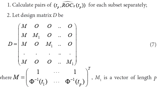
1. Calculate pairs of ( ,t ROC t_p k( ))_p for each subset separately; 2. Let design matrix D be

1 1 1 .. .. .. . . . .. . ..         =        

M O O O

M M O O

D M O M O

M O O M

(7)

where 1 1

1

1

1

( )

( )

− −





=





Φ

Φ









T p

M

t

t

, M₁ is a vector of length p

with constant value of one, and O _{is a zero value matrix.}

3. Let Y= ( , ,..., )Y Y 1 2 YK T and Yk = (Φ−1(ROC tk( ))...1 Φ−1(ROC tk( )))p ;

4. Our linear model is: for the reference subset,



1 1

1 _{1 1 1}

(ROC t( ))p β γ ( )tp ε,

− −

Φ  + Φ +

where nD,1ε1 is normally distributed with mean 0 and asymptotic

covariance matrix Σ_r,1; and for subset k,k = 2,3,..,K



1 1

1 1

(ROC tk( ))_p β γ ( )t_p β_k ε_k,

− −

Φ  + Φ + +

where nD k, εk is normally distributed with mean 0 and asymptotic

covariance matrix Σ_r,k;

5. Our OLS estimator for

θ

* _is

* 1

ˆ = (D D D Y)

θ _′ − _′

The above method assumes covariate effects can be explained adequately by the difference in the intercept parameter (α₀). If in addition we allow the slope of a binormal ROC curve to be different across covariate categories by assuming

Φ−1_(ROC

k(t)) = β1 + γ1Φ−1(t) + (1 Φ−1(t)) θTZ(k), (8)

where 2 2

=

T k k

β

β

θ

γ

γ

















then the parameter of interest is θ* _{= (β}

1, γ1,…, βk, γk)T. The estimating

procedure is similar to the case where only intercept parameters vary, but with M₁ replaced by M in (7). Inference for the significance of θ* _in

both settings can be achieved by estimating the variance of θ* _{with the}

bootstrap resampling method.

Simulation

Estimation of the ROC curve

The estimation procedure specified in the previous section starts with the choice of the false positive set T. Although in theory, any

λ α0 α1 R(0.2) R(0.4) R(0.7)

0.5 1.10 1.72 1.09 1.06 1.20

1 1.10 1.64 1.05 1.06 1.20

2 1.10 1.59 1.03 1.06 1.20

chosen set of T _{would yield estimators with the same asymptotic}

property, their small sample properties need to be investigated. An obvious starting point is to choose the collection of the observed false positive fractions that fall into the interval [a,b], we call this observed FP (OFP) method. In the case where there are no ties in the test results of non-diseased subjects, this is equivalent to the method selecting the subset of {1/ ,2 / ,...,(nD nD nD−1) / }nD within [a,b], which we call

the equal fraction (EF) method. Another possible choice is to divide interval [a,b] into nD−1 equally spaced sub-intervals and choose the midpoints of those subintervals to be the set T (midpoint(MP) method). For the last two methods, the number of points in T always equal to nD−1 regardless of the length of [a,b].

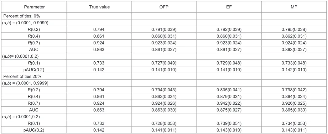
We compare the performance of the OLS estimators between those three different methods of selecting T (OFP, EF and MP). We simulate dataset both with and without ties and vary the values of [a,b] to estimate either a full curve or a partial ROC curve.

First, we generate YDN(0,1) and YDN( / ,1/α α0 1 α12)

. The resulting ROC curve follows a binormal model: ROC(t) = Φ(α₀

+ α₁Φ−1_{(t)). The parameters (α}

0, α1) are chosen to be (1.2, 0.45),

corresponding to an area under the curve (AUC) value of 0.863 and a partial AUC (pAUC) value of 0.142 for t ∈ (0, 0.2). With sample size of nD=nD= 100, we compare the biases and sampling standard errors in estimating AUC, ROC(0.2), ROC(0.4) and ROC(0.7) in the full curve estimation and pAUC(0.2) and ROC(0.1) in the partial curve estimation. To simulate data with ties, we chose 20% tied values within each population.

From Table 2, when the test results have no ties, midpoint(MP) method has the best performance. When data has ties, observed false positive fraction(OFP) method has the smallest bias when estimating the entire curve, but MP has the best performance for estimating the partial curve. We recommend using either method MP or OFP in practice and we choose MP method for the subsequent simulations (Table 2).

Next we compare performance of the OLS estimator with two

existing semiparametric ROC modeling approach (ROC-GLM and PV), which have been shown to have good performance among others. Table 3 summarizes relative biases and standard errors for the three estimators for estimating either a full or a partial ROC curve. We observe that when the full ROC curve is of interest, the OLS and the GLM estimators have comparable performances while the PV estimator has somewhat larger biases. When estimating a partial ROC curve, however, the OLS estimator can have substantially smaller bias compared to other estimators (Table 3).

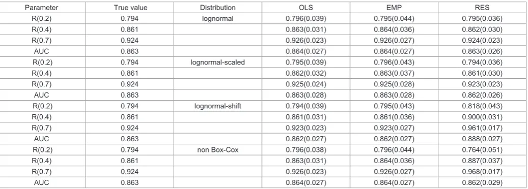
In Table 4, we demonstrate performance of the OLS estimator relative to the nonparametric ROC estimator and the parametric ROC estimator assuming normal case and control distributions after

Box-Cox transformation. We generate data as YDLOGN(0,1) and

2

0 1 1

( / ,1/ )

D

Y LOGNα α α so the resulting ROC curve is the same as

above. We further modify the data as following: (i) inflating all data points by two fold (scaled log normal distribution); (ii) increasing all data points by 2 units (shifted log normal distribution); (iii) exp(Y1/3

) (non Box-Cox). For the parametric method, Box-Cox transformation is applied to YD and YD separately before the fitting of a normal

distribution. For log normal data or scaled log normal data, the OLS estimator and the parametric estimator combined with Box-Cox transformation have similar performances. For shifted log normal and non Box-Cox data, however, the parametric estimator performs poorly with a large bias even after a Box-Cox transformation. Both the OLS estimator and the nonparametric estimator are unbiased in these scenarios with the former substantially more efficient (Table 4).

Lastly, we perform simulation studies to investigate the use of large sample inference for ROC curve and AUC based on the OLS estimator. Table 5 shows the mean estimated asymptotic error and the coverage of corresponding 95% Wald confidence intervals. The variance estimate from the asymptotic theory reflects the actual sampling variance and the coverage of 95% confidence intervals is excellent (Table 5).

Application to DPOAE Data Set

The DPOAE data set was first published by Stover et al. [13].

Parameter True value OFP EF MP

Percent of ties: 0% (a,b) = (0.0001, 0.9999)

R(0.2) 0.794 0.791(0.039) 0.792(0.039) 0.795(0.038) R(0.4) 0.861 0.860(0.031) 0.860(0.031) 0.862(0.031) R(0.7) 0.924 0.923(0.024) 0.923(0.024) 0.924(0.024) AUC 0.863 0.861(0.027) 0.861(0.027) 0.863(0.027) (a,b)= (0.0001,0.2)

R(0.1) 0.733 0.727(0.049) 0.729(0.048) 0.733(0.048) pAUC(0.2) 0.142 0.141(0.010) 0.141(0.010) 0.142(0.010) Percent of ties:20%

(a,b) = (0.0001, 0.9999)

R(0.2) 0.794 0.794(0.043) 0.805(0.041) 0.798(0.042) R(0.4) 0.861 0.862(0.034) 0.879(0.031) 0.864(0.034) R(0.7) 0.924 0.924(0.026) 0.942(0.022) 0.926(0.025) AUC 0.863 0.863(0.030) 0.875(0.027) 0.865(0.030) (a,b) = (0.0001,0.2)

R(0.1) 0.733 0.728(0.053) 0.739(0.051) 0.734(0.053) pAUC(0.2) 0.142 0.141(0.011) 0.143(0.010) 0.143(0.011)

Table 2: Inference of the ROC curve by the semiparametric least squares based method (OLS) with different choices of the false positive sets (OFP: observed false positive fraction, EF: equal fraction or MP: midpoint method). Cases and controls are drawn from normal distributions. (α0, α1) = (1.2, 0.45). n , nD D = (100, 100). Sample

Parameter True value OLS GLM PV (a,b) = (0.0001, 0.9999)

α0 1.2 1.09(0.150) 1.46(0.152) 2.40(0.161)

α1 0.45 2.42(0.083) 1.38(0.080) 9.44(0.101)

R(0.2) 0.794 -0.14(0.040) 0.16(0.038) -0.53(0.040) R(0.4) 0.861 -0.02(0.031) 0.12(0.031) 0.15(0.032) R(0.7) 0.924 -0.02(0.023) -0.002(0.023) 0.38(0.024) (a,b) = (0.0001,0.2)

α0 1.2 0.18(0.246) -1.79(0.235) 7.45(0.266)

α1 0.45 -0.62(0.141) -6.82(0.130) 14.04(0.159)

R(0.05) 0.677 0.11(0.051) 1.27(0.049) -1.00(0.051) R(0.1) 0.733 -0.02(0.046) 0.51(0.046) 0.11(0.045) R(0.15) 0.768 -0.13(0.046) 0.08(0.045) 0.61(0.045)

Table 3: Inference of the ROC curve by the semiparametric least squares based method (OLS), the ROC-GLM method (GLM) and the placement value method (PV). Cases and controls are drawn from normal distributions. (α0,α1) = (1.2, 0.45), (n nD, D ) = (100, 100). Relative bias and sampling standard error from 500 simulations are shown. Relative bias = bias/true value × 100%.

Parameter True value Distribution OLS EMP RES

R(0.2) 0.794 lognormal 0.796(0.039) 0.795(0.044) 0.795(0.036) R(0.4) 0.861 0.863(0.031) 0.864(0.036) 0.862(0.030) R(0.7) 0.924 0.926(0.023) 0.926(0.027) 0.924(0.023)

AUC 0.863 0.864(0.027) 0.864(0.027) 0.863(0.026)

R(0.2) 0.794 lognormal-scaled 0.795(0.039) 0.796(0.043) 0.794(0.036) R(0.4) 0.861 0.862(0.032) 0.863(0.037) 0.861(0.030) R(0.7) 0.924 0.925(0.024) 0.925(0.028) 0.923(0.023)

AUC 0.863 0.863(0.028) 0.863(0.028) 0.862(0.026)

R(0.2) 0.794 lognormal-shift 0.794(0.039) 0.795(0.043) 0.818(0.043) R(0.4) 0.861 0.861(0.031) 0.861(0.036) 0.900(0.031) R(0.7) 0.924 0.923(0.023) 0.923(0.027) 0.961(0.017)

AUC 0.863 0.862(0.027) 0.862(0.027) 0.888(0.027)

R(0.2) 0.794 non Box-Cox 0.796(0.038) 0.796(0.044) 0.764(0.051) R(0.4) 0.861 0.863(0.031) 0.864(0.036) 0.887(0.037) R(0.7) 0.924 0.926(0.023) 0.926(0.027) 0.968(0.017)

AUC 0.863 0.864(0.027) 0.864(0.027) 0.862(0.029)

Table 4: Inference of the ROC curve by the semiparametric least squares based method (OLS), the nonparametric method (EMP) and the parametric method (RES).

Cases and controls are drawn from log-normal distributions and modified as noted. (α0, α1) = (1.2, 0.45). (n nD, D) = (100, 100). Sample means and sampling standard errors from 1000 simulations are shown.

Relative Bias SSE ASE CP

(n nD, D) = (100, 100)

α0 2.4% 0.163 0.151 94.8%

α1 2.2% 0.085 0.083 95.4%

R(0.2) 0.4% 0.039 0.039 94.6%

R(0.4) 0.3% 0.032 0.031 93.4%

R(0.7) 0.1% 0.025 0.023 90.8%

(n nD, D) = (100, 50)

α0 0.9% 0.159 0.157 95.0%

α1 2.9% 0.088 0.088 94.6%

R(0.2) -0.3% 0.041 0.042 94.6%

R(0.4) -0.1% 0.033 0.033 94.6%

R(0.7) -0.1% 0.025 0.024 93.8%

(n nD, D) = (50, 100)

α0 1.1% 0.205 0.208 96.4%

α1 0.9% 0.101 0.113 97.2%

R(0.2) -0.2% 0.053 0.053 93.8%

R(0.4) -0.2% 0.041 0.043 94.4%

R(0.7) -0.3% 0.030 0.033 94.6%

Table 5: Result of 1000 simulations to evaluate the application of inference based on asymptotic theory to finite sample studies. (α0, α1) = (1.2, 0.45). Relative bias = bias

/ true value x 100%; SSE: sampling standard error; ASE: mean estimated standard error using asymptotic theory; CP: coverage of 95% Wald-confidence intervals using

DPOAE stands for distortion product otoacoustic emission, which is an audiology test used to separate normal-hearing from hearing-impaired ears.

The test is administrated under nine different auditory stimulus conditions with three levels of frequency (1001, 1416 and 2002 Hz) and three levels of intensity (55, 60 and 65 dB SPL). A total of 210 subjects were included in the study. The subjects were considered cases with hearing impairment at a given frequency if their audiometric threshold exceeds 20dB HL measured by a behavior test (gold standard). Each subject was tested in only one ear. Test result is the negative signal-to-noise ratio, -SNR, with higher value being more indicative of hearing impairment. The objective of the analysis is to determine the optimal setting for the clinical use of DPOAE to separate normal from hearing-impaired ears, but bear in mind an ear may be determined to be hearing impaired or normal at different frequencies.

We partition the data into nine subsets, corresponding to the nine test settings. Data is analyzed by the method specified in (8) where both intercept and slope parameters vary across subsets. The set T is chosen by the midpoint method from (0.0001, 0.9999). We choose the reference subset (subset 1) to be the test setting with frequency value of 1001Hz and intensity value of 55 dB SPL. Let (β₁, γ₁) be the intercept and slope estimates for the ROC curve for setting (1001, 55) and the subsequent β_k and γ_k, with k = 2,…,9, represent the differences in the intercept and slope parameters of the ROC curves between subset k and subset 1. None of the γˆk is statistically significantly different from 0 at

α = 0.05 α= 0.05 level (data are not shown). We also develop a χ2

test statistic γ γˆ'Σˆγˆ, where γ = (γ2,…γ9) and

ˆ_γ

Σ is the estimated covariance matrix of γˆ. Write the null hypothesis as H₀: γ = 0 and compare the above statistic with a χ2

distribution with 8 degrees of freedom gives a P-value of 0.84, suggesting insignificant slope terms consistent with the result from testing the significance of each γ_k separately.

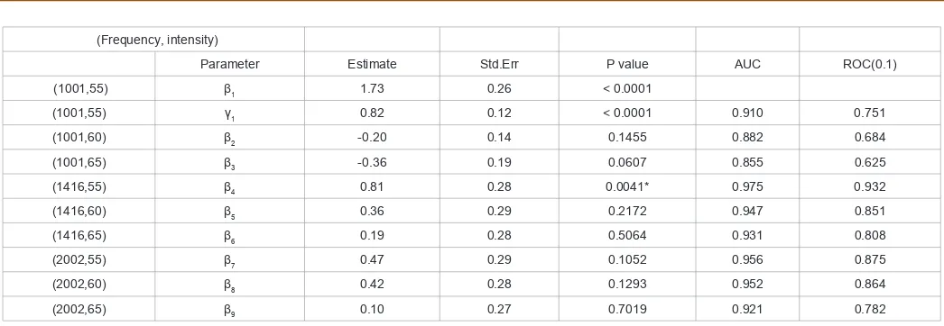
We re-analyze the data with the slope terms omitted and Table 6 summarizes the results. We can see that among the nine test settings, the setting (1416, 55) (β₄) has the largest intercept estimate and the difference from the intercept of the reference setting (1001, 55) is statistically significant (p=0.0041). The p values for other parameters (β₂ β₃ β₅to β₉₎ are not significant. The estimated ROC curve for setting (1416, 55) is ROC(t) = Φ(2.54 + 0.82Φ−1_{(t)) with estimated AUC value}

of 0.975, which is the largest among all settings. The performance of the test declines with increasing intensity at each fixed frequency value. This analysis suggests (1416Hz, 55 dB SPL) is a better test setting than the reference setting. It has also shown that at fixed false positive level of 10%, the expected sensitivities for the nine test settings range from 62.5% to 93.2%, demonstrating the importance of choosing an optimal test setting (Table 6).

Concluding Remarks

This manuscript proposes a semiparametric OLS method to estimate and compare performance of diagnostic tests and more generally, to assess potential covariate effects on the test performance. The asymptotic distribution theory for the OLS estimator is developed for the ROC curve estimation, in which the estimators are shown to be consistent and asymptotically normally distributed. For modeling covariate effects, we recommend boostrap resampling for variance estimation.

Our proposed estimator provides useful addition to the field of rank-based semiparametric ROC modeling. Those semiparametric approaches are more robust than parametric approaches, by assuming a functional form on the ROC curve itself but not the test results and thus invariant to monotone transformation of the test results. At the same time, they offer better efficiency compared to nonparametric method. We have done extensive simulations to compare the proposed OLS estimator with two other commonly used semiparametric ROC modeling methods (the ROC-GLM and placement value based method), and found the OLS estimator has comparable performance in general and slightly better performance in some scenarios [12]. The OLS estimator, however is much more intuitive compared to other estimators and very easy to implement using standard linear regression software, which could make it particularly appealing to clinical audience.

In summary, the proposed linear regression framework provides an unified approach for the ROC curve analysis. It can be used to estimate the ROC curve, as well as model covariate effect. The application of ROC curve goes beyond the medical diagnostic field and it can be used for evaluating any discrimination tools. It is, and will continue to be an important and exciting area to engage in research.

Acknowledgements

The authors would like to acknowledge Margaret S. Pepe for her invaluable contribution to the development of this manuscript. The work is partially funded by NIH grant GM54438 and P30CA015704.

(Frequency, intensity)

Parameter Estimate Std.Err P value AUC ROC(0.1) (1001,55) β1 1.73 0.26 < 0.0001

(1001,55) γ1 0.82 0.12 < 0.0001 0.910 0.751

(1001,60) β2 -0.20 0.14 0.1455 0.882 0.684

(1001,65) β3 -0.36 0.19 0.0607 0.855 0.625

(1416,55) β4 0.81 0.28 0.0041* 0.975 0.932

(1416,60) β5 0.36 0.29 0.2172 0.947 0.851

(1416,65) β6 0.19 0.28 0.5064 0.931 0.808

(2002,55) β7 0.47 0.29 0.1052 0.956 0.875

(2002,60) β8 0.42 0.28 0.1293 0.952 0.864

(2002,65) β9 0.10 0.27 0.7019 0.921 0.782

References

1. Swets JA, Pickett RM (1982) Evaluation of diagnostic systems: method from signal detection theory. Academic Press.

2. Pepe MS (2004) The statistical evaluation of medical tests for classification and

prediction. Oxford University Press, United Kingdom.

3. Metz CE, Kronman HB (1980) Statistical significance tests for binormal roc

curves. J Math Psychol 22: 218-243.

4. Metz CE, Herman BA, Shen JH (1998) Maximum likelihood estimation of receiver operating characteristic (ROC) curves from continuously-distributed data. Stat Med 17: 1033-1053.

5. Dorfman DD, Alf E (1969) Maximum likelihood estimation of parameters of

signal detection theory and determination of confidence intervals-rating method

data. J Math Psychol 6: 487-496.

6. Pepe MS (1997) A regression modelling framework for receiver operating characteristic curves in medical diagnostic testing. Biometrika 84: 595-608. 7. Pepe MS (2000) An interpretation for the ROC curve and inference using GLM

procedures. Biometrics 56: 352-359.

8. Alonzo TA, Pepe MS (2002) Distribution-free ROC analysis using binary regression techniques. Biostatistics 3: 421-432.

9. Pepe MS, Cai T (2004) The analysis of placement values for evaluating discriminatory measures. Biometrics 60: 528-535.

10. Cai T (2004) Semi-parametric ROC regression analysis with placement values. Biostatistics 5: 45-60.

11. Hsieh F, Turnbull BW (1996) Nonparametric and semiparametric estimation of the receiver operating characteristic curve. Ann Statist 24: 25-40.

12. Baker SG, Pinsky PF (2001) A proposed design and analysis for comparing digital and analog mammography. J Am Statist Assoc 96: 421-428.

13. Stover L, Gorga MP, Neely ST, Montoya D (1996) Toward optimizing the clinical utility of distortion product otoacoustic emission measurements. J Acoust Soc Am 100: 956-967.

14. Zhang Z (2004) Semiparametric least squares analysis of the receiver operating characteristic curve. University of Washington.

Submit your next manuscript and get advantages of OMICS Group submissions

Unique features:

• User friendly/feasible website-translation of your paper to 50 world’s leading languages • Audio Version of published paper

• Digital articles to share and explore

Special features:

• 200 Open Access Journals • 15,000 editorial team • 21 days rapid review process

• Quality and quick editorial, review and publication processing

• Indexing at PubMed (partial), Scopus, DOAJ, EBSCO, Index Copernicus and Google Scholar etc • Sharing Option: Social Networking Enabled

• Authors, Reviewers and Editors rewarded with online Scientific Credits • Better discount for your subsequent articles



0 1

|

( )

( ) |

0

. .

sup

e

t

ROC t

ROC t

a s

 





(9)

They also showed (Theorem 2.2) for independent observations, under the above conditions, there

exists a probability space on which one can define sequences of two independent versions of Brownian

bridges

(

B

₁( )n

,

B

₂( )n

, 0

 

t

1)

, and the following statement holds:



12

1

( ) 0 1 ( ) 2

1 1 1 2

(

( ))

(

( )

( )) =

(

( ))

( )

(

(

) )

(

( ))

n n

e D

t

n

ROC t

ROC t

B

ROC t

B

t

o n

logn

t

  













 









(10)

. .

a s

uniformly on

[ , ]

a b

,

0 <

a

<

b

< 1

.

The above two theorems stated the strong consistency and strong approximation properties for

the ROC curve.

Fix

t



[ , ]

a b

, by intermediate value theorem,





1 1 1 *

(

ROC t

e

( ))

(

ROC t

( )) = (



(

ROC t

( )))(

ROC t

e

( )

ROC t

( ))

  



 





(11)

where



*

|

ROC t

( )



ROC t

( ) | |



ROC t

e

( )



ROC t

( ) |

(12)

Therefore,

ROC t

*

( )



ROC t a s

( ) . .

by (9)

From continuous mapping theorem:

1 * 1

(

(

ROC t

( )))

(

(

ROC t

( ))) . .

a s







 





(13)

Notice

1

1 1

0 1

1

1

(

(

( ))) =

=

(

(

( )))

(

( ))

ROC t

ROC t

t





  



 





 

(14)

Then we have





1 1

1 0 1

1

(

(

( ))

(

( )))

(

( )

( ))

(

( ))

e e

D D

n

ROC t

ROC t

n

ROC t

ROC t

t

  

 





 





 

(15)

Let



1 1

( ) =

(

(

e

( ))

(

( )))

n D

V t

n





ROC t

 



ROC t

(17)

( ) ( )

1 1 2

1 1

1

1

( ) =

(

( ))

( )

(

(

( )))

(

( ))

n n

V t

B

ROC t

B

t

ROC t

t



















(18)

Equation (16) implies

V t

_n

( )



V t

( )

in (

D a b

[ , ],|| . || )

_

Equation (4) resulted from the fact that V(t) is the sum of two independent Brownian Bridges.

Appendix II: Proof of Theorems 1