The mathematics of object recognition in machine and human vision

California State University, San Bernardino California State University, San Bernardino

CSUSB ScholarWorks

CSUSB ScholarWorks

Theses Digitization Project John M. Pfau Library

2003

The mathematics of object recognition in machine and human

The mathematics of object recognition in machine and human

vision

vision

Sunyoung Kim

Follow this and additional works at: https://scholarworks.lib.csusb.edu/etd-project

Part of the Applied Mathematics Commons

Recommended Citation Recommended Citation

Kim, Sunyoung, "The mathematics of object recognition in machine and human vision" (2003). Theses Digitization Project. 2425.

https://scholarworks.lib.csusb.edu/etd-project/2425

THE MATHEMATICS OF OBJECT RECOGNITION IN MACHINE

AND HUMAN VISION

A Thesis

Presented to the

Faculty of

California State University,

San Bernardino

In Partial Fulfillment

of the Requirements for the Degree

Master of Arts

in

Mathematics

by

Sunyoung Kim

THE MATHEMATICS OF OBJECT RECOGNITION IN MACHINE

AND HUMAN VISION

A Thesis

Presented to the

Fa9ulty of

California State Uni~ersity,

San Bernardino

by

Sunyoung Kim

12--/4

!os

Oat~ I

December 2003

Approved by:

Chair

Peter William, Chair

Department of Mathematics

Terry Hallett,

Graduate Coordinator Department of

ABSTRACT

We present the framework of projective geometry. This

framework allows us to study the reconstruction of three­

dimensional structure and motion from sequences of two­

dimensional images of the available features of an object.

This theory is derived in the context of the affine camera,

which preserves parallelism and generalizes the

orthographic, scaled orthographic and para-perspective

camera models.

We derive explicit recognition polynomials for the

detection of rigid three-dimensional motion from two weak­

perspective views by using Kontsevich's equation. In

addition to detection of rigid motion, these polynomials

can be used to recognize a given three-dimensional object

from two-dimensional views,. and in fact to reconstruct its

depth coordinates.

We also provide some interesting theorems in linear

algebra which arise as generalizations of theorems used in

ACKNOWLEDGMENTS

I thank God for the intellect to explore the wonderful

world of Mathematics. I thank my parents for give me a

support and opportunity to study in United State of

America. I thank Paul Amaya, who is assistant director of

International Student Services, for helped me and

understood me about my situation and legal status. Most of

all, I thank my advisor Dr. Chetan Prakash for his patient

TABLE OF CONTENTS

ABSTRACT i i i

CHAPTER FOUR: RECOGNITION OF RIGID THREE DIMENSIONAL MOTION FROM SEQUENCES OF TWO

CHAPTER FIVE: RECONSTRUCTION OF THREE DIMENSIONAL MOTION FROM SEQUENCES OF TWO

ACKNOWLEDGMENTS iv

LIST OF FIGURES vi

CHAPTER ONE: PROJECTIVE GEOMETRY 1

CHAPTER TWO: CAMERA MODELS . . . 5

CHAPTER THREE: EPIPOLAR LINES AND PLANES 15

DIMENSIONAL IMAGES . . . 20

DIMENSIONAL IMAGES . . . . 26

CHAPTER SIX: SOME THEOREMS IN LINEAR ALGEBRA 28

LIST OF FIGURES

Figure 1. Image Formation in a Pinhole Camera 5

Figure 2. The Pinhole Camera Model . 6

Figure 3. Camera Models: (a) perspective (all rays

pass through a single projection point O,

and the intersection of the ray star with

the image plane _generates the image); (b) orthographic(all rays are parallel, with the optical center Oat infinity);

(c) weak perspective(combined orthographic

and perspective projection). For (b) and

(c), parallel lines in the scene remain parallel in the image; this isn't true for

(a). 10

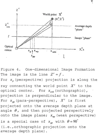
Figure 4. One-dimensional Image Formation

The image is the line

zc

=

f'.

xP (perspective) projection is along the

ray connecting the world point Xe to the

optical center. For xonh (orthographic) ,

projection is perpendicular to the image.

For xPP (para-perspective) , Xe is first

projected onto the average depth plane at

angle 0, and then projected perspectively

onto the image plane; x~ (weak perspective)

is a special case of xPP with 0=90° (i.e.,

orthographic projection onto the average

depth plane) 11

Figure 5. The Epipolar Geometry 15

Figure 6. (Ci,C_{2 )} is Parallel to the Plane R_{1 :}

is oo; the epipolar lines are parallel

E₁

in the plane R₁ and at intersect at E₂

17

Figure 7. (Ci,C2 ) is Parallel to the Planes R1

CHAPTER ONE

PROJECTIVE GEOMETRY

The study of projective geometry is related to the

sort of sensors that machines and humans use for vision.

It is known from geometric optics that any system of lenses

can be approximated by a system that realizes a perspective

projection of the world onto a plane. The simplest way to

look at such a system is to look at i t projectively. Here

is the general definition of projective space of any

dimension.

Definition: a point of an n dimensional real projective

is represented by an (n+l) vector of real coordinates

x= [ Xi,X 2 ,···,xn+I], where at least one of the xi is nonzero.

The numbers are called the homogeneous or projective

coordinates of the point, and the vector x i s called a

coordinate vector. Note that the correspondence between

points and coordinate vectors is not one to one.

Note that an (n+l) x (n+l) matrix A such that det(A)-::f:-0

defines a linear transformation on Rn+I _{which may be}

'

interpreted as a projective isomorphism ofP11

Definition: i) (n+l)x(n+l) matrix A with detA:;cO is called

a collineation. ii) the set of collineations is a group and

this group is also known as the projective group. iii) a

projective basis is a set of (n+2) points of pn such that

no (n+l) of them are linearly dependent. Any point x of

pn can be described as a linear combination of the (n+l)

points of the standard basis:

n+I

x = Ix;e;'

i=l

where X; are the projective coordinates in this basis.

P1

For n

=

P

is called the projective plane;

P

is called simply

P1

projective space. The space is the simplest of all

projective spaces and many structures embedded in

higher-dimensional projective spaces have the same structure as

P1

• In P1, a point on the line can be written as x =

P2

The space is used to model the image plane as a

P2

projective plane. A point in is defined by three

numbers(xi,x₂,x_{3 ) ,} not all zero. There are objects other by

and the lines form coordinate vectors x and u defined up to

3

a scale factor. The equation of the line is then 'z:u;X;

=

P

in the standard projective basis of • Formally, there is

no difference between points and lines in P2 • This is

known as the principle of duality. Among all possible

lines, the one whose equation is x₃= 0 is called the line at

infinity of P2, denoted by

t .

3

the projective plane of the form of 'z:u;X; = 0 intersects l"'

i=l

at the point (-u₂ ,ui,O), which is the point at infinity of

the line L.

There is a structure of the projective plane that has

numerous applications, especially in stereo and motion:

P

Definition: A pencil of lines is the set of lines in

P2

passing through a fixed point. Any pencil of lines in

is projectively isomorphic to the one-dimensional

projective space P' .

P 3

A point x in , known as the projective space, is

defined by four numbers (~'~'~'~), not all zero. There

planes. A plane is also defined as a four numbers

( u"u2,u3, u4 ) , not all zero. . The points and the planes form a

coordinate vector x and u defined up to a scale factor.

4

The equation of this plane is then

I:Uixi

i=l

projective basis ( ei,e₂,e₃,e_{4 ,} e_{5 )} of P 3 • A line is defined as

the set of points that are linearly dependent on two points

and P₂ • Among all possible planes, the one whose P₁

equation is x₄ = 0 is called the plane at infinity or ~ 00 of

P 3 • As in the case of the projective plane, i t is often

useful to think of the points in the plane at infinity as

the set of directions of the underlying affine space. For

example, the point of projective coordinates [x1 , x2 , x3 , OJ

represents the direction parallel to the vector [x_{1 ,} x_{2 ,} x₃]

and indeed i t does not matter whether.x1 , x2 and x3 are

defined up to a scale factor, since the direction does not

CHAPTER TWO

CAMERA MODELS

There is a deep relationship between camera models and

projective geometry. So I would like to look at camera

models. A simple camera model can be considered from two

sta6dpoints. One is a geometric model and the other is

physical model. In this paper, we are only interest in a

geometric model.

~-•_-~

---/ /

/1

- - - image

object

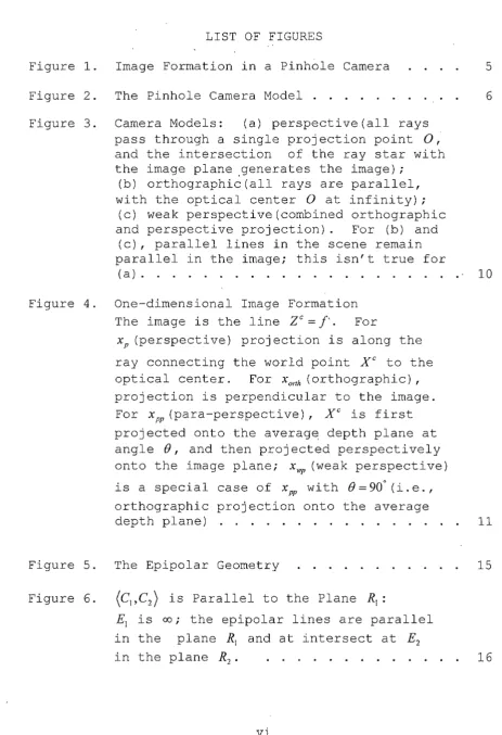
Figure 1. Image Formation in a Pinhole Camera

Let us considir the system consists of two screens. In the

first screen, a small hole has been punched and through

this bole some rays of light reach on the second screen.

---

---

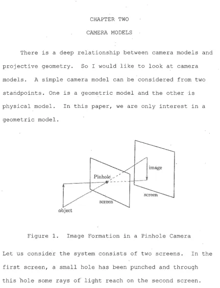
---camera that consists of a plane

R,

in which the image is formed through an operation called a

perspective projection: The distance f from the optical

center C to the retinal plane R is called the focal length

of the camera.

lvI

Figure 2. The Pinhole Camera Model

This is used to form the image m in the retinal plane of

the three-dimensional point M as the intersection of the

line CM with the plane R.

Let us take a look at camera model in further detail.

We can choose the coordinate system X = ( Xi,X2 ,X3 ) for the

3D space and x

= (

system X = ( Xi,X₂ ,X_{3 )} is called the standard coordinate

system of the camera. The relationship between image

coordinates x and 3D space coordinates can be written in

terms of a projection matrix P

Pi2 Pi3

lP,,

P,,

j

x,

(1) P2, P22 P23 P24

X3 P31 P32 P33 P34

X4

related to x and X by x

X

Thus a camera can be considered as a system that

performs a linear projective transformation from the

P3

P

projective space into the projective plane • We

sometimes refer to the three-dimensional coordinate system

X as the world coordinate system. Also, the camera can be

considered as a system that depends upon both intrinsic and

extrinsic parameters. Intrinsic parameters are those that

do not depend on the position and orientation of the camera

scale factors a 11 and av and the coordinates u0 and v0 of the

intersection of the optical axis with the image plane.

There are six extrinsic parameters, three for the rotation

and three for the translation of the camera, which define

the transformation from the world coordinate system to the

coordinate system of the camera.

There is a special case of the projective camera

called the affine camera. This affine camera can be

written using equation (1) with P31

=

=

=

Fi2 Fi3

[P.1

P,,1

pa.ff= ~ I P22 P23 P24 (2)

0 0 P34

It corresponds to a projective camera with its optical

center at the plane at infinity; consequently, all

projection rays are parallel. We can decompose PaJJ •

Gil G12 Gl3 Gl4

C12

c1,ff

G21 G22 G23 G24

[c"

Paff= CP 11 G= C21 C22 c23 o 1 0

G31 G32 G33 G34

c31 C32 C33 0 0 0

~1

G41 G42 G43 G44

The 3x3 matrix C accounts for intrinsic camera parameters

and represents a 2D affine _transformation (hence

=

C31

=

0

f

0

where~ is the camera aspect ratio, f the focal length and

(ox,oy) the principal point (where the optic axis intersects

the image plane). The 3x4-matrix Pn performs the parallel

projection operation, and the 4x4 matrix G accounts for

extrinsic camera parameters, encoding the relative position

and orientation between camera and the standard coordinate

system. Therefore the affine camera covers the composed

effects of i) a 3D affine transformation between world and

camera coordinate system; ii) parallel projection onto the

image plane; and iii) a 2D affine transformation of the

image.

In terms of inhomogeneous image world coordinates, the

affine camera is written

x

=

p

where M=

l

J

=

34

t

major property of the affine camera is that i t preserves

parallelism: lines that are parallel in the world remain

parallel in the image.

(o) (b\

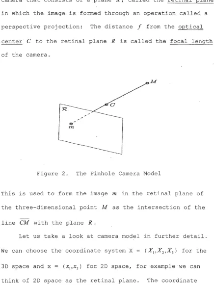
Figure 3. Camera Models: (a) perspective (all rays pass through a single projection point 0, and the intersection of the ray star with the image plane generates the image); (b) orthographic (all rays are parallel, with the optical center Oat infinity) ; (c) weak perspective (combined orthographic and perspective projection). For (b) and (c), parallel lines in the scene remain parallel in the image; this isn't truefor (a).

I would like to introduce some special cases of the

perspective projection, and para-perspective projection

cameras.

The

parallel

onto the

orthographic projection camera is modeled by rays

to the optical axis projected orthographically

average depth plane

zc=

Wot1d point Xi: (X~ Z

1

Average depth '"ptn.ne'' f Image "plane" Optical cent.re ,, ; -..

Figure 4. One-dimensional Image Formation The image is the line

zc

=

For xP (perspective) projection is along the ray connecting the world point Xe to the optical center. For x₀,.₁h ( orthographic) ,

projection is perpendicular to the image. For x~ (para-perspective), Xe is first projected onto the average depth plane at angle 0, and then projected perspectively onto the image plane; x~ (weak perspective)

Next, we look at the weak perspective projection

camera. Consider the familiar camera centered perspective

equations, where each point is scaled by its individual

depth

z~

center:

In above equation, Xe= (

Xe,Ye,ze)

camera frame. When the camera field of view is small and

the depth variation of the object ~

Zt

=

Zt -z;.,e

compared to the average distance of the object from the

camera

z;ve,

zt

Z~, giving a weak perspective or scaled orthographic

camera:

We can say the weak perspective camera is a combination of

the orthographic and perspective projection. Coordinates

measured in a world coordinate system (X) are related to Xe

translation vector representation the origin of the world

frame. The depth of a point Xi measured along the line of

sight in the camera frame is then Zt

=

of the point set is denoted

x_

the object is given by jj_ZiC

=

X

y

z

1

Next, we look at para-perspective camera. The

para-perspective camera generalizes weak para-perspective case, such

that projection of the scene point onto the average depth

plane occurs parallel to the optic axis by projecting

direction. Since the average depth plane remains parallel

to the image plane, the perspective projection stage simply

introduces a scale factor. The lD case takes the form

Xpp

=

~

zave

where 0 denotes the angl~ between the projection direction

and the positive X-axis. In the 2D case, the projection

in the X-Z plane and 0Y is the equivalent angle in the

Y-Z

the rigid transformation between the camera and world

coordinate frames gives

cot0x! cot0Y

CHAPTER THREE

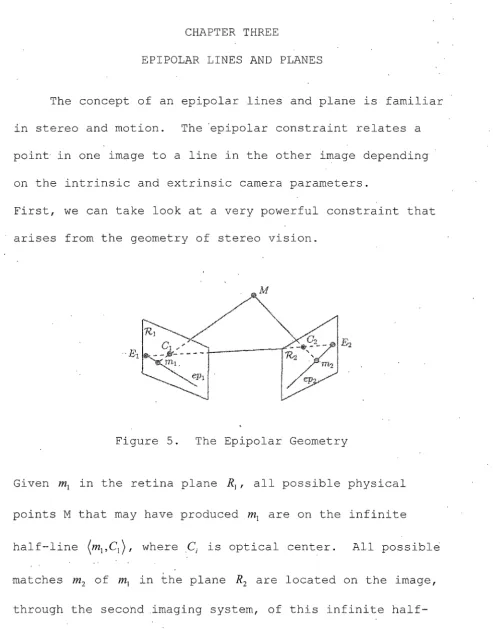
EPIPOLAR LINES AND PLANES

The concept of an epipolar lines and plane is familiar

in stereo and motion. The ·epipolar constraint relates a

point in one image to a line in the other image depending

on the intrinsic and extrinsic camera parameters.

First, we can take look at a very powerful constraint that

arises from the geometry of stereo vision.

Figure 5. The Epipolar Geometry

Given m₁ in the retina plane R_{1 ,} all possible physical

points M that may have produced m1 are on the infinite

half-line (mi,C1) , where .Ci is optical center. All possible

half-lirie. This image is an infinite half-line ep2 going through

the point E2 , which is the intersection of the line (Ci,C2 )

with the plane R_{2 •}

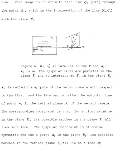
Figure 6. (Ci,C_{2 )} is Parallel to the Plane R_{1 :}

is oo; the epipolar lines are parallel in the E₁

plane R₁ and at intersect at E₂ in the plane R₂ ,

is called the epipole of the second camera with respect

E₂

to the first~ and the line ~ ₂ is called the epipolar line

of point m₁ in the retinal plane R₂ of the second camera.

The corresponding constraint is that, for a given point m1

in the plane

R

R

lies on a line. The epipolar constraint is of course

symmetric and for a point m₂ in the plane R_{2 ,} its possible

matches in the retinal plane R1 all lie on a line ep1

line (Ci,C_{2 )} with the plane R_{1 •} The lines ep₁ and ePz are the

intersections of the plane C₁MC_{2 ,} called the epipolar plane

defined by M, with the planes R₁ and R₂ , respectively.

E₂ at

00

Figure 7.

(c

R, and R2 : E1 and E2 are at oo; the epipolar lines are parallel in both planes R₁ and R₂ •

When the plane

R

R

the line (Ci,C2 ) , one or both epipoles go to infinity and the

epipolar lines in one plane or both become parallel. The

situation where both planes are parallel to the line (C1,C2)

is often assumed because of its simplicity. Let's compute

the epipolar geometry. In this section, the notation~ is

to indicate projective quantities. For example, x denotes

multiplicative nonzero scalar, and x denotes a vector of

Rn. Let mi'= P1 M and m2

=

coordinates of the two optical centers, C, (i= 1,2), in the

world reference frame, are obtained by solving the

following two systems of linear equations: P,M= 0, where

i

=

Since each epipole E₁ is the image by the ith camera of the

other camera's optical center C₁ ( j

*

coordinates of the epipoles Ei are obtained by applying

matrices PI to the vectors C 1 ( i, j = l , 2 , i

*

Now, I like to show how, for a given point m₁ in the plane

R_{1 ,} the corresponding epipolar line ep1 can be computed. We

need to points to determine a line. One of them is the

- - [ P,-1 ]

epipole E_{2 ,} which is given by e2

=

point is the point at infinity of the optical ray

(C

The image m2 of this point in the second retinal plane is

- ~

written a Fm1 where Fis a 3x3 matrix. If we let E2 be

the 3x3 antisymmetric matrix representing the cross product

with e2 • We have F

=

• Any pixel m₂ on the epipolar

~ T

line ep2 of m1 satisfies the equation m2 F m1

=

in particular that the roles of m1 and m2 are symmetric and

that the epipolar line of a pixel m₂ in the first retinal

CHAPTER FOUR

RECOGNITION OF RIGID THREE DIMENSIONAL MOTION FROM

SEQUENECS OF TWO DIMENSIONAL IMAGES

A recognition polynomial is a polynomial in the image

data (i.e., the coordinates of the points in the given

view) that evaluates to zero when the image data are

consistent with those from.rigid motions of a given 3-D

object. Using a Kontsevich's approach, we can derive

explicit recognition polynomials for the detection of rigid

3-D motion from two weak-perspective views. I would like

to introduce Kontsevich's derivation of the two-view

rigidity constraint in weak perspective projection.

Kontsevich used some of the same geometric ideas as in

Koenderink and van Doorn, notably the decomposition of

rigid rotation into a rotation about the viewing direction

and a rotation about an axis in the image plane. The

motions we consider are rigid rotations in 3-D space or

translations along the viewing direction that followed by

uniform scaling so we can ignore translations parallel to

Suppose we have an object that has five distinguished

points, labelled "0, 1, 2, 3, and 4." Let

0

displacement in

R

O

first view (with j =1, 2, 3, 4) . Then

r;

corresponding displacement, in R3 , in the second view. And

let ff be the orthographic projection to the image plane,

then the projected displacement can be written

R3 The fact is given an image plane, any rigid rotation in

can be thought of as a composition of two rotations. The

first is.a rotation about a unit axis vector v parallel to

the image plane and second is a rotation about an axis

vector perpendicular to the image plane. The second

rotation takes the first axis vector v to a new unit vector

v1 in the image plane. If the uniform scaling factor is s,

1

1 1

then we can let V = - V .

s

Consider the first of the decomposed rotations, around the

axis v. Then the respective projections of

0

v are equal and the second rotation takes v to v1• If we

denote 7z-(r))

=

p),

1

p}

same as those rigid of~ and p₁ onto v. Thus p₁ ·v=p₁ I ·v. I

Finally, consider the scaling. Since 7l" is orthographic,

the scaling factor of s results in p~=~} and, in equation

v'=!v

, we can arrive at the linear Kontsevich equations:

s

0

P1 ·V-P1I ·VI

= '

with

llvll =l, llv'JJ =

M,

IIP'JI =silPII ·

s

The equation p₁ -v-p~·v'=0 is a homogeneous system of four

linear equations in the four unknown coordinates c_1, c_{2 ,}

c;,

If we let p₁ =

[;J ,

=

coefficient matrix have rank less than 4. Thus v and v' can

be known only up to an overall scale factor; choosing a

factor s from the equation

llv'II

=

M.

s

exposition of Kontsevitch's two-view derivation.

Now, take look at how a recognition polynomial arises

for the two-view weak perspective recognition of rigid

motion. This is a polynomial in the 16 data values

{ x₁ ,y₁ ,x:,y:} _{J=l, ...,4} which must evaluate to zero for there to be

a rigid interpretation. The condition that equation

p₁ · v-p: · v'

=

determinate of the coefficient matrix vanish. Ignoring the

negative signs in the last two columns of this matrix, we

get:

X1

Y1

X2

Y2

Y2

det =0

X3

Y3

Y4

Therefore the two-view recognition polynomial is the

determinant in above.

The recognition polynomial is a polynomial in 16 variables,

corresponding to the image plane coordinates of the weak

perspective projections of four feature points in each of

the two views. To use the polynomial for the detection of

actual object with, say, five feature points, an observer

can choose one of the points. Then, if the image

coordinates of the four remaining feature points in the two

views satisfy the recognition polynomial, we may infer that

the 3-D motion is rigid with probability one. To use the

polynomial for the recognition of a given object, suppose

we know the image plane coordinates of five feature points

on the object. We can use these coordinates to assign

numerical values to those variables in the polynomial which

correspond to the first view. This gives a reduced

polynomial in eight variables. Then, given a view of a

novel object with four feature points, we can plug the

image plane coordinates of these points into the reduced

polynomial, and if the result is 0, we may infer that the

novel object coincides with the memory object with

probability one.

Theorem: Let A be a 4x4 matrix with rank 3. Let A be the

3x4 matrix obtained from A by deleting the last row. Let

A; be the ith column of A.

cI

= -

I - -

-cI

= -

is a nontrivial solution to Ax= 0. Moreover, if both of

the 2x2 diagonal minors of A are nonsingular, then in this

I I

solution both vectors ( c"c_{2 )} T and ( c₁ ,c_{2 )} T are nonzero.

Lemma: Let A(k) be the 3 x 4 matrix obtained from A by

deleting the kth row. Let·C(k) be the vector (c₁,c₂ ,c₁ ,c₂ )T

I I

obtained from A(k) as C = (c"c₂ ,c₁ ,c_{2 )} T is from A . Then C is a

CHAPTER FIVE

RECONSTRUCTION OF THREE DIMENSIONAL MOTION FROM SEQUENCES OF TWO DIMENSIONAL IMAGES

Kontsevich performed a change of.coordinates so as to

simplify the depth reconstruction. To this end, define

A - ~ I

ev,

=

(c1

A A A A

Thus eu,ev,ez (where ez is the unit vector perpendicular to

the image plane) forms an orthogonal coordinate system, as

A A A

does _e11,,ev',ez.

A I A

Now define the u coordinates in the new systems:

11 -C2XJ +C1Y1

Note that the v,v I

coordinates, defined similarly, are equal

for corresponding points. Now let the z-coordinate of the

edge r be r₁,z • For each angle

a,

1

. ) (P1,11J

P~,_11,

= (

rJ,=

=

Hence

r₁,z

=

Letting ,1,

=

=

CHAPTER SIX

SOME THEOREMS IN LINEAR ALGEBRA

Euler's Theorem: Any RE S0(3) can be written R = R;RJ'R;,

where (¢,0,lf/) are Euler angles of R and R: is a rotation

through angle¢ around the·positive Z-axis.

S2

Proof: Let n be the north pole of • If BE S0(3) with

Bn =Rn, set C

=

i.e., C is a rotation about Bn (and Rn).

Now 30 such that R%n has the same latitude as Rn and 3¢

such that R;, (R%n) = Rn . (:.we can set R;,R%=B)

i.e. , R

=

I\ I\ I\

Lemma: If A is a rotation about r and Br= u, for some

I\

rotation B then BAB-1 is a· rotation about u.

I\

Proof: (BAB-1_{)u = BAB-}1_Br

I\

=BAJr

I\

=BAr

I\

=Br

I\

As a consequence, we can say that any rotation C about

u

=

since by the lemma, A= B-1CB is a rotation about r

=

Then C

=

Now with R =CB, ( B

=

Bn(= Rn), we have that C

=

=

Finally R

=

B

=BD

Theorem: Let A be a 3x3 matrix with rank 2. Let A be the

3x3 matrix obtained from A by deleting the last row. Let

A; be the ith column of A.

Then the vector C = ( c₁ , c₂ , c₃ ) T defined by

c₁ = -det ( A 2 , A 3 )

c₂ = det ( A 1 , A 3 )

is a nontrivial solution to A x

=

Proof: Expanding the determinant of A off the nth row, we

-a31det(A 2,A 3J + _{a 32} det(A 1,A 3 J - _{a 33} det(A 1,A 2 l= 0,since A has

rank less than n. That is, a₃₁ c₁ +a₃₂ c₂ +a₃₃ c₃ = 0.

Thus the vector C

= (

By the theory of determinants C is orthogonal to all the

rows of A, i.e., is a solution to Ax= 0.

Moreover, since A has rank exactly 2, C can not be the zero

vector. I.I

Let's check if AC= 0.

12 13 a11c1 + a c 2 + a c 3

+

+

-a31C1 + a32C2 + a33C3

l

all a12 a13

a21 a22 a23

n,

=

a31 a32 a33

- 2 - 3 -1 - 3 - \ - 2

- a11 det(A ,A )+a12 det(A ,A ) - a31 det(A ,A )

- 2 - 3 - \ - 3 -1 - 2

- a21 det(A ,A )+a₂₂ det(A ,A _{) - a32} det(A ,A)

- 2 - 3 - 1 - 3 - J - 2

- a 31 det(A ,A ) + a 32 det(A ·, A )-a 33 det(A , A )

If 2x2 minors of A are nonsingular than in this solution

vectors c;'s are nonzero.

Let c₁

=

Since C =J:. 0 and we are assuming c₁

=

nontrivial solution to 3x3 system. This contradicts 2x2

minors of A are nonsingular. Therefore c₁ =J:. 0. A similar

argument holds for c₂= 0 and c₃ = 0. Thus c;'s are nonzero

Theorem: Let A be a nxn matrix with rank n-1. Let A be

the (n-l)xn matrix obtained from A by deleting the last

row. Let A; be the i th column of A . Then the vector C =

... , en) T defined by

c₁ = -det (

A

, A 3 , A 4 , ••• , A 11 )

A 11

=

, A 3 , A 4 , ••• , )

C 2

c3

=

CI. = (- 1) ; d et ( A

1

f A

2

f ••• f A i-1 f A i+l f ••• f A)

A 2 , A n-1)

en= (-1) ndet ( A 1 ' A 3'

,

is a nontrivial solution to A x

=

Proof: Expanding the determinant of A off the nth row, we

get

- 2 - 3 An A' A3

n A I A 2 A n-1

(-1) anndet( , , .•. I )= 0, since A has rank less than n .

That is, a111c,+an2C2+ •.. +a1111cn= 0.

Thus the vector C

= (

row A11 • By the theory of ~eterminant C is orthogonal to

all the rows of A, i.e., is a solution to Ax= 0.



Let's check if AC= 0.

0

G11C1 + G12C2

+

+

G21C1 + G22C2 + G23C3 • • • + Gz,,C11

- 2 - 3 - 1 1 - I - 3 - n - J - 2 -n-1

det(A ,A , ... ,A )+a₁₂ det(A ,A , ... ,A )+ ... +(-1)11

det(A ,A , ... ,A )

-a11 a111

- 2 - 3 - n - I - 3 - n - I - 2 -n-1

-a₂₁ det(A ,A , ... ,A )+a₂₂ det(A ,A , ... ,A )+ ... +(-1)11

det(A ,A , ... ,A ) a211

- ? - 3 - n - I - 3 - n - I - ? -11-I

det(A-,A , ... ,A )+a det(A ,A , ... ,A )+ ... +(-l)"a det(A ,A-, ... ,A )

-a111 112 1111

=

Theorem: Let A be a 4x4 matrix with rank 2. Then we

provide a general algorithm for finding a basis of the null

Proof: Let B be the row-reduced matrix obtained from A .

Rearrange if necessary so that the last two rows of B are

zero.

all Ql2 G13 al4

G21 G22 G23 G24

0 0 0 0

0 0 0 0 X1

X₂

X3

X4

=

Let B be the 3x4 matrix obtained from

- ;

last row. Let B be the ith column of

0

0

0

0

B by deleting its

B. The null set of

A and B are identical (subject to the rearranging

described above), so i t suffices to find solutions to

Bx= 0 . Solutions can be found as follows.

If we let x4 =0, then the solution will be

-2 -3

= det(B ,B ) =

x1 a12 a23 -a13a22 -1 - 3

= -det(B ,B ) = -(aua23

x2 -a13 a21 )

- ] - 2

x3 = det(B ,B ) = aua22 -aI2 a21 )

If we let x₃ =0, then the solution will be

- 1 - 2 =-det(B ,B) =

If we let x₂ =0, then the solution will be

- 3 - 4

=

=

x₁ a13 a24 -a14 a23

- I - 3

=

=

x₄ a11 a23 -a13 a21

If we let x₁ = 0, then the solution will be

- 3 - 4

=

=

x₂ a13 a24 -a14 a23

In each case it is verified by direct computation that the given vector is a solution.

The question is: are any of these vectors non-trivial?

Since B has rank 2, at least one 2x2 sub-matrix of the

matrix consisting of the first two rows has to be nonzero

(since the matrix has rank 2 and any other 2x2 sub-matrix

has automatically zero determinants).

By inspection of the solutions given above, we see that

this particular 2x2 determinant, whatever i t is, appears in

two distinct vectors, both of which are therefore non­

trivial.

Furthermore, these two vectors must be linearly

other. Thus they form a basis of the two-dimensional

REFERENCES

1. Oliver Faugeras, Three-dimensional computer vision: a geometric viewpoint. Massachusetts Institute of Technology press, 1999

2. M. Brady, L. s. Shapiro, and A. Zisserman, "Three­ dimensional motion recovery via affine epiploar

geometry." Internation Jounal of Computer Vision, 16, 147-182 (1995)

3. B. M. Bennett, D. D. Hoffman, and C. Prakash,