Assessment of Vietnam’s capacity and commitment to ratify and implement the International Convention on Oil Pollution Preparedness, Response and Co-Operation (OPRC), 1990

(1)

World Maritime University

The Maritime Commons: Digital Repository of the World

Maritime University

World Maritime University Dissertations Dissertations

2016

An application of a simulation technique on rail

container transport between Laem Chabang Port

and Inland Container Depot Ladkrabang, Thailand

Ud Tuntivejakul

World Maritime University

Follow this and additional works at:http://commons.wmu.se/all_dissertations

This Dissertation is brought to you courtesy of Maritime Commons. Open Access items may be downloaded for non-commercial, fair use academic purposes. No items may be hosted on another server or web site without express written permission from the World Maritime University. For more information, please [email protected].

Recommended Citation

Tuntivejakul, Ud, "An application of a simulation technique on rail container transport between Laem Chabang Port and Inland Container Depot Ladkrabang, Thailand" (2016).World Maritime University Dissertations. 529.

(2)

WORLD MARITIME UNIVERSITY

Malmö, Sweden

AN APPLICATION OF A SIMULATION

TECHNIQUE ON RAIL CONTAINER TRANSPORT

BETWEEN LAEM CHABANG PORT AND INLAND

CONTAINER DEPOT LADKRABANG, THAILAND

By

Ud Tuntivejakul

Kingdom of Thailand

A dissertation submitted to the World Maritime University in partial

Fulfilment of the requirements for the award of the degree of

MASTER OF SCIENCE

In

MARITIME AFFAIRS

(PORT MANAGEMENT)

2016

(3)

ii

DECLARATION

I certify that all the material in this dissertation that is not my own work has been identified, and that no material is included for which a degree has previously been conferred on me.

The contents of this dissertation reflect my own personal views, and are not necessary endorsed by the University.

(Signature):

(Date): 19th September 2016

Supervised by: Devinder Grewal World Maritime University

Assessor: Ilias Visvikis

Institution/organization: World Maritime University

Co-Assessor: Gerhardt Müller

(4)

iii

ACKNOWLEDGEMENTS

First of all, I would like to express my gratitude to the Port Authority of Thailand and Laem Chabang Port for providing me an opportunity to expand knowledge of maritime affairs, especially, Dr. Yohei Sasakawa, the chairman of the Nippon Foundation who provided a full scholarship for me to study at World Maritime University.

My appreciation also goes to my distinguish professor, Professor Dr. Devinder Grewal, who monitored my dissertation work, provided advice and suggestions which led me to completion.

Special thanks to the director of Port Operation Division, Mr. Veerachart Phuttaraksa, and all members of the division who provide valuable information. Thanks to Mr. Siripong Koomprapan, Chief,Marketing and Development Freight Division of the State Railway of Thailand and Mr. Khomkit Puttarat of Hutchison Ports (Thailand) Limited who gave the vital information for this dissertation.

I would like to thank my senior students from my country Surasak Changjul and Sirirath Thepanual, who helped me settled down during the first period of study at World Maritime University. Thanks to my classmates Pitinoot Kotcharat, Aditya Srivastava, Thet Wai Lynn Htut, Alexandros Tsalavoutas, and Avinash Kumar, who always supported me during my dissertation progress.

(5)

iv

ABSTRACT

Title of Dissertation: An Application of a Simulation Technique on Rail Container Transport between Laem Chabang Port and Inland Container Depot Ladkrabang, Thailand

Degree: Master of Science

Since the increasing demand of container transport through Laem Chabang Port, Thailand, the port faces landside congestion due to the large share of road transport. The Inland Container Depot Ladkrabang is the dry port facility to support and increase the efficiency, and ease the congestion at the port by linking the dry port and the seaport by rail; however, the share of transport between the two facilities is largely by road.

There are three modes of transport at Laem Chabang Port i.e. road, rail, and barge. The large share of a modal split by road creates severe landside congestion. Moreover, the Inland Container Depot Ladkrabang, which serves the direct rail link to Laem Chabang Port has a larger share of road transport. This causes traffic congestion from the increasing container throughput and other problems, i.e. air emissions, pollution in port and local community, excess cost of transport, and road accidents.

This dissertation aims to study the reason why the modal share by rail has not increased, which hinders the growth of the rail transport between the two facilities by rail container transport data analysis. Furthermore, the research studies the effectiveness of government policies and investment into the rail transport system between Laem Chabang Port and Inland Container Depot Ladkrabang. Finally, the simulation technique is utilized using Rockwell Software Arena 14 to generate the virtual model, which is based on the real world system parameters and characteristics.

The virtual simulation model allows free configurations and adjustments based on the real world applicability. Three scenarios are assumed, constructed, and quantified by the software. The results show that there are possibilities to create more efficient systems in the virtual models. The presentation of the real world application shows how the virtual model could be implemented and which measures are required to maintain the system efficiency. This also illustrates the impact of the system application to the current situation.

(6)

v

LIST OF TABLES

Table 1. Rail transfer charges of LCP... 28

Table 2. Financial analysis scenario 1 ... 35

Table 5. Container throughput of ICD from 2012-2015 ... 38

Table 6. Simulation results of the current state ... 69

Table 7. Scenario 2 train schedule ... 71

Table 8. Scenario 3 train schedule ... 74

Table 9. Simulation results of Scenario 1 ... 77

Table 10. Simulation results of Scenario 2 ... 78

(11)

x

LIST OF FIGURES

Figure 1 Import and export process. ... 7

Figure 2 Share of commodity cargo by rail freight transport (millions tons), 2014. ... 8

Figure 3 SRT rail network. ... 9

Figure 4 The location of Laem Chabang Port... 10

Figure 5 Layout of Laem Chabang Port. ... 11

Figure 6 The location of ICD Ladkrabang... 14

Figure 7 Container throughput of ICD and LCP. ... 16

Figure 8 Containers transported by rail at ICD... 17

Figure 9 Percentage of the modal split between rail and road at ICD. ... 18

Figure 10 Percentage of the modal split between rail and road at LCP... 19

Figure 11 Overview of the container handling operation between ICD and LCP. ... 22

Figure 12 Layout of ICD. ... 23

Figure 13 Layout of Laem Chabang Port rail yard areas. ... 24

Figure 14 Breakdown of domestic freight transportation, 2014. ... 27

Figure 15 The modal split of LCP, 2015. ... 29

Figure 16 Policy implementation and investments by government on rail transport. ... 30

Figure 17 Annual operating cost of container handling equipment... 32

Figure 18 Break down of annual operating cost of reach stacker. ... 33

Figure 19 Unimodal alternatives (road and rail). ... 43

Figure 20 Multimodal transport (road and rail). ... 44

Figure 21 Comparison of a conventional transport and an implemented dry port concept. ... 45

Figure 22 Histogram of number of wagons each trip from ICD to LCP. ... 51

Figure 23 Histogram of number of wagons each trip from LCP to ICD. ... 52

Figure 24 Histogram of the amount of time that locomotives spend at LCP. ... 52

(12)

xi

Figure 26 Histogram of delay time from ICD to LCP. ... 54

Figure 27 Histogram of delay time from LCP to ICD. ... 55

Figure 28 Proportion of rail freight transport by day... 56

Figure 29 Container share of gate operators at ICD. ... 56

Figure 30 Container share of terminal operators at LCP. ... 57

Figure 31 Simulation process. ... 59

Figure 32 Diagram of the system. ... 60

Figure 33 Components of the model... 61

Figure 34 Analysis procedure. ... 62

Figure 35 Distribution of inter-arrival time ICD to LCP. ... 63

Figure 36 Distribution of inter-arrival time LCP to ICD. ... 64

Figure 37 Addition of calculation formulas to the model. ... 66

Figure 38 Rail container transport between ICD and LCP simulation in Arena 14. ... 68

Figure 39 Details of transit time. ... 72

Figure 40 Layout of Laem Chabang station ... 73

Figure 41 Comparison of the current system and the Scenario 3 system. ... 75

Figure 42 Comparison of simulations results. ... 80

Figure 43 Comparison of the actual modal spilt and theoretical modal spilt of ICD (2015). ... 83

(13)

xii

LIST OF ABBREVIATIONS

The following abbreviations are used in this dissertation:

ICD Inland Container Depot Ladkrabang LCP Laem Chabang Port

(14)

1

CHAPTER 1: INTRODUCTION

1.1 Background

International trade of Thailand has been growing continuously. The Lehman Brothers crisis in 2009 and floods in 2011 slowed down the international trade and had an impact on Thailand’s economy. Even though, the growth of international trade is still steadily increasing afterward.

Since the introduction of containerized cargo transport, the volume of containerized cargo has risen steadily (UNESCAP, 1999). Credit should be given to the standardization of container boxes, which allows fast, easy, and secure handling. The boxes are compatible to mount on vehicles, trailers, and rail wagons, which make multimodal transport operation run smoothly and efficiently. The benefits of the standardization of containers increase the popularity of containerized cargo transport across the globe, thus increasing the containerized cargo volume (Ham & Rijsenbrij, 2012).

(15)

2

hand, the negative effects are congestion on both landside and the seaside due to increasing traffic, throughput and overcapacity (Jaržemskis & Vasiliauskas, 2007). Laem Chabang Port (LCP) is a major seaport in Thailand. Starting the operation in 1991 with the continuously growing cargo volume, the port became the gateway of Thailand’s international trade. Inland Container Depot Ladkrabang (ICD) is the supporting facility of LCP. ICD acts as a dry port in order to ease the congestion at LCP by providing a railway link to transport containers to and from both facilities. However, there is growing landside congestion due to a large amount of container traffic transported by road at LCP and ICD. Despite having the rail container handling facilities and daily operation of rail container transport, the share of road transport is still very large. The large share of the road transport causes an impact on the surrounding community around the port, environmental problems, excessive budget for road maintenance, and congestion.

1.2 Objectives

There is a growing congestion at LCP since the port has a continuously growing throughput. Most of the day, there are several long truck queues outside the terminal gates. In the peak day, each truck could wait up to many hours due to the large share of a modal split by road. Meanwhile, at ICD, due to the low share of a modal split by rail transport, the traffic congestion at ICD is also severe.

As aforementioned, the objective of ICD is to promote an environmentally friendly and fuel efficiency mode of transport. This also helps reducing the landside congestion by transporting containers by rail instead of transporting by road; however, the objective of the ICD has not been met due to the modal split by rail is a lot lower than an modal split by road. Therefore, there is a growing congestion situation in both ICD and LCP.

(16)

3

 Identify the system constraints or bottlenecks of the rail container transport between ICD and LCP, which hinder the system efficiency.

 Quantify the potential capacity of the system.

 Present the alternatives and possible changes in the system to improve system efficiency.

 Present the measures to apply the virtual experiment to the real world system.

1.3 Methodology

The author has used methods to conduct this research according to the following steps.

Step 1: By acquiring knowledge and collecting information in order to identify useful knowledge for the topic. Relevant articles have provided a basic overview of rail freight transport in Thailand in general.

Step 2: By doing a literature review – there are many best practices or multimodal transport problem cases. The author has used some of these methods as a tool to find a suitable way to solve this problem.

Step 3: By identification of the operation process in order to find the constraints or bottlenecks, which might hinder the system efficiency.

Step 4: Applying simulation techniques by using discrete event simulation software (Arena 14) to mimic the rail container transport system between ICD and LCP.

Step 5: Apply configurations and adjustments to the model in order to see the potential capacity and efficiency of the system.

(17)

4

1.4 Contribution of this research

Obviously, the rail transport between ICD and LCP is inefficient. This research will observe a bottleneck in the system and present the practical means of operation to improve the system efficiency. Without any empirical experiment, the study will be conducted by using simulation software. The concept of this study is to observe the effects of the system modification in order to quantify and assess the results of the modification. It should be noted that each modification will be examined by scenario.

The idea in each scenario will contribute to the further empirical testing on the real system, thus, improve the system efficiency.Other benefits from efficient rail transport are road congestion reduction, which is an environmentally friendly promotion by using more energy efficient mode of transport, accident reduction from a less congested road, and increasing the port competitiveness by improving the hinterland connection efficiency.

The simulation model can contribute to future research on the rail freight transport between ICD and LCP or can be utilized in other rail transport systems since the model can be modified and adjusted according to the different system parameters.

1.5 Layout of dissertation

(18)

5

(19)

6

CHAPTER 2: RAIL FREIGHT TRANSPORT IN THAILAND

2.1 Rail freight transport

Rail freight transport is an economical mode of transport on land, which can carry a large volume of cargo in the concept of economy of scale. This creates a competitiveness, energy saving, and causes low pollution (Armstrong, 1978). Rail freight transport, which involves two or more modes of transport or so-called multimodal transport, will be explained further.

2.2 Multimodal transport

(20)

7

Import and export process

Figure 1.

Source: The author

2.3 Overview of rail freight transport

(21)

8

Share of commodity cargo by rail freight transport(millions tons), 2014

Figure 2.

Source: Adapted from State Railway of Thailand

As seen in Figure 2, the containerized cargo contributes mostly in the total rail freight transport of Thailand and most of the traffic happens between ICD and LCP.

(22)

9

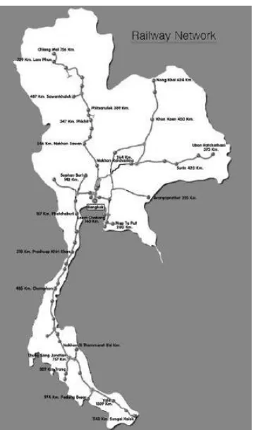
SRT rail network

Figure 3.

Source: www.railway.co.th

2.5 Laem Chabang Port

(23)

10

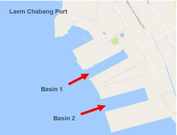
Due to the increasing volume of cargo handled by the port, the phase two development began in 1997 and was completed in 2000. Two of the so called basins were dredged to the depth of 16 meters along with deepening the entrance channel and breakwater extension to 1,900 meters.

The location of Laem Chabang Port

Figure 4.

(24)

11

Layout of Laem Chabang Port

Figure 5.

Source: Adapted from Google maps

LCP operates under the Port Authority of Thailand (PAT), which is under the supervision of the Ministry of Transport of Thailand. It is the major deep sea port of Thailand, which can accommodate up to post panamax ships and provides various kinds of maritime transport services. The port uses the landlord model, so PAT supervises the overall infrastructure including approaching channel maintenance dredging, water supply, electricity supply, access to the port (roads and lighting), port entrance gates, navigational aids, tug boats, and mooring line handling. On the other hand, the port has given concession agreements to private operators to handle the operation, for instance, construction of the superstructure, purchasing of the handling equipment, cargo operation, maintenance of the terminal area, and personnel recruitment. The maritime transport services are provided by the terminal operators as follows:

(25)

12

 Roro terminals (1 terminals)  Passenger terminals (1 terminal)  General cargo terminals (1 terminal)  Shipyard (1 yard)

The port gave concessions to major shipping lines and terminal operators, which are AP Moller, Evergreen, PSA, MOL, NYK, DP World, and HPH who are responsible for the terminals’ operation and also some other areas for rent to other private or governmental agents, which are private companies, Industrial Estate of Thailand, Customs Bureau, Animal and Plant Quarantine Agency, Dangerous Cargo Warehouse, which have supporting or connecting operations to the port. The port is associated with 14 terminals categorized by letter A, B, and C according to the series of terminals and the harbor basins. The list of terminal operators are as follows:

 LCMT Co, Ltd. (A0 Terminal)

 NYK Auto Logistics Co., Ltd. (A1 Terminal)

 Thai Laem Chabang Terminal Co., Ltd. (A2 Terminal)

 Hutchison Laem Chabang Terminal Co., Ltd. (A3 and C1-2 Terminal)  Aawthai Warehouse Co., Ltd. (A4 Terminal)

 Namyong Terminal Public Company Limited (A5 Terminal)  LCB Container Terminal 1 Co., Ltd. (B1 Terminal)

 Evergreen Container Terminal (Thailand) Co., Ltd. (B2 Terminal)  Eastern Sea Laem Chabang Terminal Co., Ltd. (B3 Terminal)  TIPS Co., Ltd. (B4 Terminal)

(26)

13

2.6 Inland Container Depot Ladkrabang

Supporting the port operations, the Inland Container Depot Ladkrabang (ICD) was built in 1996. The inland container depot or so-called dry port is a concept of easing the congestion in the seaports to inland facilities. The cargo volume is transferred to the dry port allowing ports to better utilize the area. The dry port also acts as a hub for intermodal transport by linking through the ports by rail or road (Roso et al., 2009)

In 1989, Japan International Cooperation Agency (JICA) cooperated with the Thai government to make a feasibility study regarding to the construction of the inland container depot to support the operation of LCP. Hence, the ICD was constructed.

(27)

14

The location of ICD Ladkrabang

Figure 6.

Source: Adapted from Google maps

Objectives of the construction and operation of ICD are as follows:

 Facilitate the import/export activities.

 Promote the usability of LCP by reducing the tariff between ICD and LCP.  Support the planning policy of the Bangkok port congestion reduction.  Environmentally friendly and fuel efficiency promotion.

(28)

15

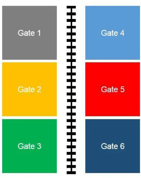
 Siam Shoreside Services Ltd. (Gate 1) (SSS)

 Eastern Sea Laem Chabang Terminal Co., Ltd. (Gate 2) (ECCO)  Evergreen Container Terminal (Thailand) Co., Ltd. (Gate 3) (ECTT)  TIFFA ICD Co., Ltd. (Gate 4) (TIFFA)

 Thai Hanjin Logistics Co., Ltd. (Gate 5) (THL)

 NYK Distribution Service (Thailand) Co., Ltd. (Gate 6) (NYK)

The distance of rail connection from ICD to LCP is 118 kilometers; the track is meter gauge type, the average speed of the rolling stock is around 40 kilometers/hour, and the transit time is nearly three hours. There are on average 24 trips of trains/day. Each trip carries 37 wagons and each wagon carries two TEU of containers; the rail operation between ICD and LCD involves containerized cargo only. From 1996 to 2012, the railway from Ladkrabang to Laem Chabang station was single track and from 2012 to present after the transport and logistics promotion policy of Thailand by the Ministry of Transport, SRT constructed double track railway to enhance the track capacity; however, the connection from the Laem Chabang station to the rail yards inside LCP area is around 4 kilometers and is still single track.

There are rail yards in LCP to accommodate the container throughput from ICD. In the export operation, once the wagons are all fully loaded from ICD, the rolling stock spends nearly three hours from ICD to LCP then stops at the rail yard. The container handling is performed by the terminal operators in LCP. For the import, the containers are unloaded from the ship and transferred to the rail yard. The containers will be loaded by the terminal operators onto the rail wagons, and once the train has been unloaded, it will travel back to ICD.

(29)

16

unstuffed at ICD for final delivery; LCP also imports empty containers to supply ICD for export cargo.

2.7 Statistics of the container handled in ICD and LCP

The following section shows the statistics of the container handled at ICD and LCP in order to show some analysis which leads to the objective of the study.

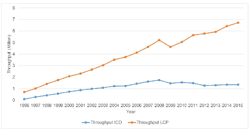
Container throughput of ICD and LCP

Figure 7.

(30)

17

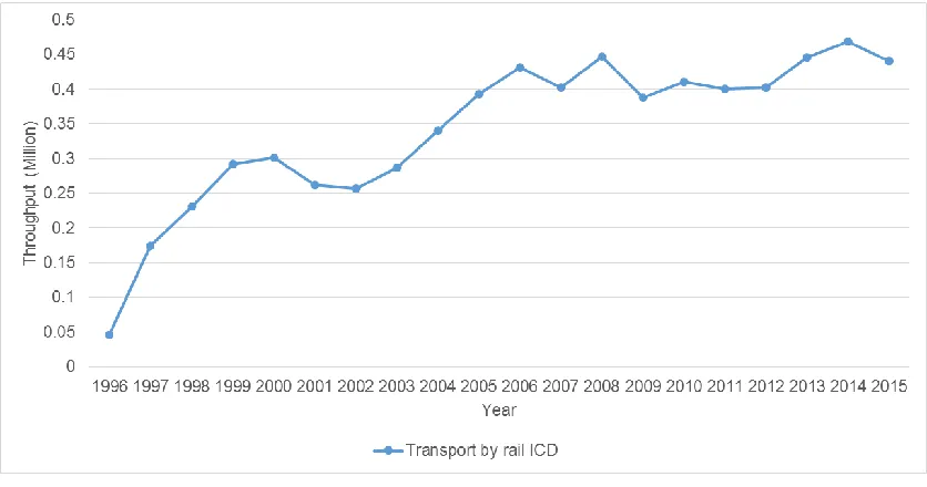
Containers transported by rail at ICD

Figure 8.

(31)

18

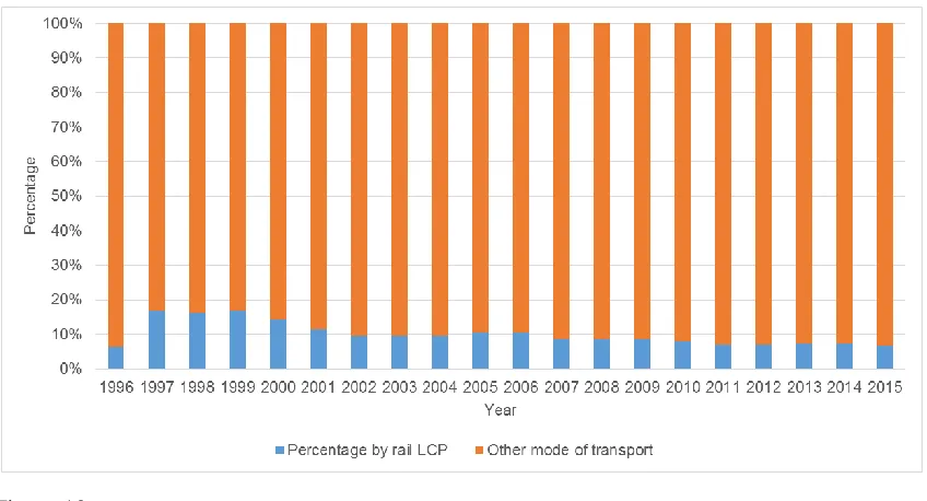
Percentage of the modal split between rail and road at ICD

Figure 9.

(32)

19

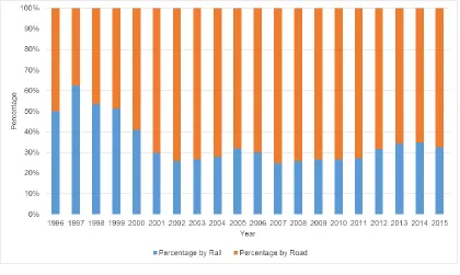
Percentage of the modal split between rail and road at LCP

Figure 10.

Figure 10 shows the percentage of the modal split by rail at LCP. The percentage of rail containers has been declining since 1999 due to the growing volume of containers at LCP whereas, the capacity of ICD has been fully utilized since 2000.

2.8 Import and Export processes

This section explains the detail of rail freight operation, which links between ICD and LCP. There are details of import and export processes, layouts of the operational area and limitations of freight transport.

2.8.1 Import process

(33)

20

operator at LCP is informed, requesting the containers to be handled at the rail yard for further transport. The shipping line also informs the module operator in ICD to arrange the wagon booking for the containers. The wagon booking should be done by the module operator by informing SRT in the daily meeting, which is conducted to share the wagons among operators. Since there are six module operators, conflict of interest happens due to limited resources of SRT (there are 24 trips of trains per day and each train carries 37 wagons, with a capacity of 74 TEU). Once the daily meeting is done, the wagon proportion of that meeting should be the share of wagons for the following day; hence, the request from the consignee should be done in advance.

Once the ship has arrived at the port, the unloading operation is performed by the terminal operators at LCP, and then the terminal operators will transfer the containers to the rail yard. The duty of the consignee or the shipping line is to make a declaration form to the customs office called “customs permission of transport cargo by other modes of transport”. The concept behind this document is that the customs office has set up a control area called customs limit in order to prevent smuggling of cargo or transport of containers out of the customs limit without customs release order. However, the customs permission of transport cargo by other modes of transport enables the transporter to make a customs release order at the point of discharge, in this case, at ICD. The terminal operators have to ensure that the documentation is done before loading the containers to the rail wagon. Once the containers are loaded into the wagon, SRT will transport the wagon by a locomotive to the ICD, where the containers will be unloaded by the module operators for further delivery.

2.8.2 Export process

(34)

21

plan to make a wagon booking in the daily meeting with SRT. Once the wagon request is confirmed, the module operators will send the confirmation to the shipping line and contact the terminal operators in LCP with a notice about container arrival. After that, the container will be transported to the container yard at LCP and transferred to the terminal by the terminal operators and wait to be loaded onto the ship.

2.9 Operation details and layouts

SRT is responsible for the rail freight operation between ICD and LCP by making concession agreements to module operators to conduct the cargo handling operation. The locomotives and wagons are also managed by SRT. Within the ICD premises, there are government agents who regulate to the import and export procedures, namely Customs Bureau, Quarantine Office, and Food and Drugs Agency.

The distance between ICD and LCP is 118 kilometers, and there are 24 trips/day, 12 of which are from ICD to LCP for export containers and another 12 trips are from LCP to ICD for import containers. The track is meter gauge, and the distance 114 kilometers to the Laem Chabang station is 114 kilometers with double tracks and the remaining 4 kilometers within LCP area is single track.

(35)

22

Overview of the container handling operation between ICD and LCP

Figure 11.

Figure 11 gives the big picture of the operation overview. In more details of the loading/unloading operations, there are tally and inspection and cargo handling together within 60 minutes, and within 30 minutes, there are disconnecting and connecting of locomotive and wagons including general safety checking.

The export process is the process whereby containers are transported from the container yards by reach stackers and loaded onto the truck chassis at ICD. The truck will deliver the containers to the apron beside the track and the container will be lifted and loaded onto the rail wagon. Once the containers are transported to LCP, unloading is performed by reach stackers and then the containers will be loaded to the truck chassis at the rail yard before moving to the terminal area by terminal trucks. The containers are then stacked in the container yard by Rubber Tired Gantry Cranes (RTG).

(36)

23

containers are transported by the rolling stock to the rail yards at ICD for further direct delivery or being unstuffed before delivery.

The layout of the operational areas of both ICD and LCP in order to provide the general understanding of the movement of containers, locomotives, and freight wagons is shown as follows:

2.9.1 ICD’s Layout of the operational areas

Layout of ICD

Figure 12.

Source: The author

(37)

24

equipment (mainly reach stackers, empty handlers, and terminal truck), and cargo handling equipment (mainly forklifts).

Rolling stocks travel through the middle of all gates, and gate operators bring reach stackers to operate loading and unloading operations at the apron in front of the track Delivering or receiving cargo and containers is performed at the terminal gates on the opposite side of the apron.

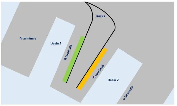
2.9.2 LCP’s Layout of the operational areas

Layout of Laem Chabang Port rail yard areas

Figure 13.

Source: The author

(38)

25

In the export process, once the train has arrived, terminal operators dispatch reach stackers to load and unload containers and temporarily store them at the rail yards before moving to the terminal. In the import process, terminal operators transfer the containers to the rail yards by truck for temporary storage before loading them onto the rail wagons by reach stacker.

2.10 Limitation of rail freight transport

There are limitations which constrain or disallow importers, exporters, and forwarders to transport containers by rail as follows.

 Refrigerated container limitation – Currently, there is no refrigerated container reception equipment installed in the wagon. For that reason, importers, exporters, and forwarders have to transport refrigerated containers by truck. There are some refrigerated containers handled at ICD, and these containers are all transported by truck.

 Dangerous cargo container limitation – Currently, there are no limitations in the transport of dangerous goods by rail. However, according to LCP regulations, for safety reasons, all dangerous goods have to be handled, stored and managed by the designated company, which is the expert in handling dangerous goods. Therefore, once the containers have arrived at LCP, the containers have to be directly transferred to a Dangerous Cargo Warehouse within the port area. This causes additional charges involving the transfer of containers. Consequently, the total cost of transporting dangerous cargo is no longer less expensive than direct transport by truck from the point of origin.

 Container Security Initiative1 (CSI) by U.S. Customs and Border Protection – In case a container has been randomly picked for scanning according to CSI, the

1_{CSI addresses the threat to border security and global trade posed by the potential for terrorist use of a maritime}

(39)

26

container has to be transferred to the scanning facilities within the port area prior to being loaded on to the ship. This causes additional charges involving the transfer of containers. Consequently, the total cost of the scanned container is more expensive than direct transport by truck from the point of origin. However, the CSI performs the task on a random basis; therefore, there is around a 5% chance subject to the probability and exporter profiles.

 There is weight limitation of the wagons, carrying capacity of the wagons ranging from 24-38 tons; therefore, sometimes the heavy 20” containers are carried on only one wagon due to loading of another 20” container with a significant weight difference which can cause an accident due to instability. There is 25% of rail wagons transported between ICD and LCP carrying only one TEU.

2.11 Policies, strategies, plans and projects to improve the capacity and efficiency of

the rail freight services

A major strategy proposed by the government to reduce the cost of transport is to reduce the share of road transport and shift to rail and barge transport. In the perspective of the Ministry of Transport, rail transport is an efficient means of transport as it is environmentally friendly, and helps reducing road congestion, road accident, and logistics cost. Thailand has a very high percentage share of road transport; however, very low rail transport as shown in Figure 14.

(40)

27

Breakdown of domestic freight transportation, 2014

Figure 14.

Source: Adapted from Ministry of Transport

(41)

28

Table 1. Rail transfer charges of LCP

Items 20" 40" More than 40"

Import Container

FCL / LCL 690 (US$20) 1,040 (US$30) 1,110 (US$32)

Empty 250 (US$7) 370 (US$11) 400 (US$12)

Export Container

FCL / LCL 520 (US$15) 780 (US$22) 830 (US$24)

Empty 250 (US$7) 370 (US$11) 400 (US$12)

Note: The charges cover the transfer of FCL2, LCL3 or empty containers from the container yard to the rail yard and also the loading of containers on the rail wagons in the case of import container or vice versa, the currency is in Thai Baht (THB).

Source: Laem Chabang Port

The charges were reduced to 470 Baht (US$14) and finally to 315 Baht (US$10) for all container status in 2004. This strategy attracted shipping lines, importers, exporters, and forwarders to utilize rail transport as the main mode of container transport between ICD and LCP due to the cost being lower than road transport after the reduction of tariffs.

Moreover, there is a privilege for the containers which use other modes of transport (coastal vessel or barge and rail) rather than road announced by LCP. This policy stated that containers which utilize coastal vessels or barges and rail transport should have only one hour closing time4. This gives a high flexibility for the exporters and forwarders, who are responsible for delivering the containers to the terminal compared to road transport whose closing time is 24 hours.

2_{FCL is a container shipment which loaded and sealed at origin by single supplier or manufacturer, then shipped by a}

combination of ocean, road or/and rail to final destination (https://cargofromchina.com/fcl-lcl/).

3_{LCL is container shipment which loaded by multiple suppliers or manufacturers, this allows exporters to ship smaller}

amounts of cargo that is not of a large enough volume to make FCL a viable option. This means the container is combined with many shipping consignments headed for the same destination (https://cargofromchina.com/fcl-lcl/).

4_{Closing time is the limit of a time window for a container to be delivered to terminal prior to the berthing of the ship}

(42)

29

Apart from the container handling charges’ reduction, infrastructure improvement projects are also introduced. There are five categories: double tracking, track rehabilitation, new network expansion, upgrading of signaling, and telecommunication systems. The major improvement between ICD and LCP was double tracking which was completed and has been fully in operation since 2012. This provides unlimited track capacity and eliminates waiting time from shunting.

Moreover, SRT also purchased new locomotives for replacing aging ones to improve the operations in 2015; therefore, the carrying capacity has been increased from 30 wagons to 37 wagons per locomotive.

Despite having many major improvements and investments in the operations, rail freight transport has not improved considerably because the major mode of container transport of LCP is still dominantly carried out by road according to Figure 15.

The modal split of LCP, 2015

Figure 15.

Source: Adapted from Laem Chabang Port

(43)

30

2.12 Examination of the effects of the government policies and investments on rail

freight transport

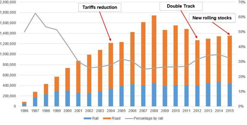
This section shows the effectiveness of the government’s policies, strategies, and plans/projects intended to improve the capacity and efficiency of the rail freight services. As aforementioned, the Ministry of Transport has been supporting the modal shift from road to other modes of transport in order to reduce the logistics cost, environmental impacts, and congestions. A series of policy implementations and investments have been done as follows:

Policy implementation and investments by government on rail transport

Figure 16.

(44)

31

Word boxes and red arrows point out the implementation of policy and investments on the certain points of time. As seen in 2004, in order to attract importers, exporters, forwarders, and shipping lines to use rail freight transport, tariff reduction policies were announced. In 2012 and 2015, double track construction and purchasing of new locomotives were performed respectively.

In 2004, after the reduction of prices, the ICD throughput went up dramatically to its peak in 2008 (nearly 1.8 millions TEU). However, the upward trend was seen as a large share of road transport rather than rail.

The drop in 2009 was the consequence of the global financial crisis. Since then the throughput remains steady until the present. The construction of double tracks and purchasing of the new locomotives did not generate a significant increase in container throughput.

2.12.1 Tariffs reduction strategy

Implemented in 2004, the tariffs have reduced to 315 Baht (US$10) for all containers and status transported by rail to LCP. This section is to investigate how effective the strategy implementation is.

(45)

32

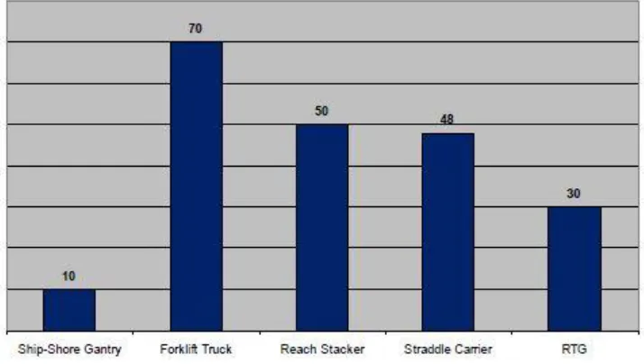
Annual operating cost of container handling equipment

Figure 17.

Source: World Bank

The data from the World Bank shows that the annual operating cost of reach stackers is approximately 50% of the purchasing price.

(46)

33

Break down of annual operating cost of reach stacker

Figure 18.

Source: World Bank

Assumptions of the financial analysis of the rail container operation:

 Fixed cost

Reach stacker costs analysis: Purchasing prices of reach stackers is approximately 600,000 USD or around 18,000,000 Baht. For the efficient operations, there are two reach stackers; therefore, the cost of a reach stacker is 36,000,000 Baht. Depreciation of the reach stacker should be estimated by the straight line method through the economic life cycle of 10 years: 2,880,000 Baht.

Operating cost

(47)

34

 Variable cost

Fuel: According to the World Bank, the annual fuel price is around 10% of the purchasing price i.e. 1,260,000 Baht. There are three scenarios in the assumption that the fuel cost should vary, plus or minus 20% according to the number of containers handled.

 Revenue

The assumption of the revenue is based on the number of containers handled. According to statistics, the author will make 3 assumptions (handling of containers of 20,000, 30,000, and 40,000 boxes), the tariff per box is 315 Baht (US$10); however, due to the fact that the rail yards are the property of LCP; therefore, it is LCP’s policy to deduct 15 Baht (US$0.5) for each box for the common use of the rail yards as the budget for maintenance and operational lightings. Then, the net revenue of the terminal operator is 300 Bath (US$9.5) /box.

 Indicator of the analysis is the annual profit and loss of the operations.

(48)

35

Table 2. Financial analysis scenario 1

Scenario 1 analysis: Handling 20,000 boxes of containers annually, fuel consumption of 1,008,000 Baht/year. The result shows a loss every year.

0 1 2 3 4 5 6 7 8 9 10

Initial Cost 36,000,000

Fixed Cost

Depreciation 2,880,000 2,880,000 2,880,000 2,880,000 2,880,000 2,880,000 2,880,000 2,880,000 2,880,000 2,880,000

Operating cost 12,600,000 12,852,000 13,109,040 13,371,221 13,638,645 13,911,418 14,189,646 14,473,439 14,762,908 15,058,166

Total Fixed cost 15,480,000 15,732,000 15,989,040 16,251,221 16,518,645 16,791,418 17,069,646 17,353,439 17,642,908 17,938,166

Variable Cost

Fuel 1,008,000 1,008,000 1,008,000 1,008,000 1,008,000 1,008,000 1,008,000 1,008,000 1,008,000 1,008,000

Total Variable cost 1,008,000 1,008,000 1,008,000 1,008,000 1,008,000 1,008,000 1,008,000 1,008,000 1,008,000 1,008,000

Total Cost 16,488,000 16,740,000 16,997,040 17,259,221 17,526,645 17,799,418 18,077,646 18,361,439 18,650,908 18,946,166

Revenue 6,000,000 6,000,000 6,000,000 6,000,000 6,000,000 6,000,000 6,000,000 6,000,000 6,000,000 6,000,000

(49)

36

Scenario 2 analysis: Handling 30,000 boxes of containers annually, fuel consumption of 1,260,000 Baht/year. The result shows a loss every year.

0 1 2 3 4 5 6 7 8 9 10

Fixed Cost

Depreciation 2,880,000 2,880,000 2,880,000 2,880,000 2,880,000 2,880,000 2,880,000 2,880,000 2,880,000 2,880,000

Operating cost 12,600,000 12,852,000 13,109,040 13,371,221 13,638,645 13,911,418 14,189,646 14,473,439 14,762,908 15,058,166

Total Fixed cost 15,480,000 15,732,000 15,989,040 16,251,221 16,518,645 16,791,418 17,069,646 17,353,439 17,642,908 17,938,166

Variable Cost

Fuel 1,260,000 1,260,000 1,260,000 1,260,000 1,260,000 1,260,000 1,260,000 1,260,000 1,260,000 1,260,000

Total Cost 16,740,000 16,992,000 17,249,040 17,511,221 17,778,645 18,051,418 18,329,646 18,613,439 18,902,908 19,198,166

Revenue 9,000,000 9,000,000 9,000,000 9,000,000 9,000,000 9,000,000 9,000,000 9,000,000 9,000,000 9,000,000

(50)

37

Scenario 3 analysis: Handling 40,000 boxes of containers annually, with a fuel consumption of 1,512,000 Baht/year. The result shows a loss every year.

0 1 2 3 4 5 6 7 8 9 10

Fixed Cost

Depreciation 2,880,000 2,880,000 2,880,000 2,880,000 2,880,000 2,880,000 2,880,000 2,880,000 2,880,000 2,880,000

Operating cost 12,600,000 12,852,000 13,109,040 13,371,221 13,638,645 13,911,418 14,189,646 14,473,439 14,762,908 15,058,166

Total Fixed cost 15,480,000 15,732,000 15,989,040 16,251,221 16,518,645 16,791,418 17,069,646 17,353,439 17,642,908 17,938,166

Variable Cost

Fuel 1,512,000 1,512,000 1,512,000 1,512,000 1,512,000 1,512,000 1,512,000 1,512,000 1,512,000 1,512,000

Total Cost 16,992,000 17,244,000 17,501,040 17,763,221 18,030,645 18,303,418 18,581,646 18,865,439 19,154,908 19,450,166

Revenue 12,000,000 12,000,000 12,000,000 12,000,000 12,000,000 12,000,000 12,000,000 12,000,000 12,000,000 12,000,000

(51)

38

2.12.2 Double track construction

Table 5. Container throughput of ICD from 2012-2015

Year Throughput Rail throughput Road throughput Percentage by rail

2012 1.271 0.402 0.869 32%

2013 1.301 0.446 0.855 34%

2014 1.344 0.468 0.876 35%

2015 1.355 0.44 0.915 32%

Note: Throughput shown in millions TEU.

Double track construction was fully functional in 2012. Table 5 shows statistics of container throughput of ICD between 2012 and 2015. There are very marginal increases in throughput from year to year and also minor changes in the percentage of rail throughput.

2.12.3 Purchasing of new locomotives

New locomotives were purchased in 2015 to replace all of the old models; consequently, the efficiency of the operations improved from the transport of 30 wagons to 37 wagons each trip. It is expected to be up to a 25% increase in container throughput.

2.13 Chapter summary

(52)

39

(53)

40

CHAPTER 3: LITURATURE REVIEW

3.1 Logistics concept

(54)

41

inbound, outbound, internal, and external movements, and return of materials for environmental purposes” (Reference: Council of Logistics Management, http://www.clm1.org/mission.html, 12 Feb 98). “The process of planning, implementing, and controlling the efficient, cost-effective flow and storage of raw materials, in-process inventory, finished goods and related information from point of origin to point of consumption for the purpose of meeting customer requirements” (Reference: Canadian

Association of Logistics Management,

http://www.calm.org/calm/AboutCALM/AboutCALM.html, 12 Feb, 1998). There are many other definitions, which provide similar or near similar meanings, and as mentioned, it can be summarized that logistics is the cargo and information movement management in such an efficient and cost-effective manners. The main focus of the logistics is time and cost which can be derived as 3R’s consists of Right thing, at the Right place, at the Right time; on top of the 3R’s can be Right price, Right customer, Right condition, and Right quantity. (Class notes, Port logistics and planning, World Maritime University, 2016).

3.2 Port performance and competition

(55)

42

There are factors regarding the port competition as explored by Yuan et al. in 2011. There are three groups of port users, who are shipping lines, forwarders, and shippers. By using the Analytic Hierarchy Process (AHP) to the industry experts, it found that, the factors considered in this study are port location, costs at port, variety of rates, port facility, storage space, shipping services, terminal operators, port information system, electronic information, hinterland connection, customs, and government regulations. The results showed that the most important factor for the shipping lines is costs at port (terminal handling fees and other expenses), followed by customs and government regulations and hinterland connections. In the perspective of forwarders, the most important factor is port location, followed by hinterland connection. In the viewpoint of shippers, port location is the most important factor. From the empirical results, it is illustrated that hinterland connection is not the most important factor for all the port users; however, among the top ranking factors, it is the significant factor to consider and could be one of the influential elements for the port competitiveness.

3.3 Comparative analysis of road and rail transport

(56)

43

Unimodal alternatives (road and rail)

Figure 19.

Source: Adapted from Jonkeren et al. (2011)

(57)

44

Multimodal transport (road and rail)

Figure 20.

Source: Adapted from Banomyong and Beresford (2001)

With the cost at the multimodal transfer point, the rail transport cost curve shifts upward and becomes a multimodal transport cost curve. Examples of the transfer costs are handling costs, terminal fees, and surcharges (Banomyong & Beresford, 2001). This makes the break-even point move to longer distance.

3.4 Dry port concept

(58)

45

Comparison of a conventional transport and an implemented dry port concept

Figure 21.

Source: Roso (2009)

As seen in Figure 21, instead of transport by point to point from the cargo origins to the seaport as (a), all the points of transport are concentrate at the dry port, which directly links to the seaport as (b), resulting in shorter transport route, more energy efficient mode of transport, and less congestion for roads and city (Roso, 2009). However, this generates higher cargo handling cost than the additional cargo handling has at the dry port.

3.5 Rail freight transport challenges and solutions in other literature

This section is a review of relevant literature and articles. Books or articles are shown in the sub-topics and the brief description, methodology, and summary is explained in the following.

3.5.1 Hinterland connectivity of Malaysian container seaports: Challenges and

solutions

(59)

46

There are problems of imbalance of a modal split (98% transported by road and 2% transported by rail), road congestion, space constraint in dry port, emission and environmental problems from road transport, service reluctance of trucking companies over the short distance, and limitation in rail transport due to track capacity (single track). Interviews were used to find the problems, solutions, and recommendations.

Chen et al., (2015) has summarized that in order to improve the efficiency of Malaysian transport infrastructure, responsible agencies need to develop the following guidelines:

 Improve rail infrastructure to electrified double tracks.  Improve the quality of wagons.

 Improving the trade corridor by improving rail facilities and cargo services.  Reduce haulage cargo formalities.

 Moving non-maritime activities away from the seaport.  Deploy traffic polices to check overload trucks.

 Road expansion.

 Dry ports provide haulage services to deliver the container to the destination.  Joint collaboration among dry ports for efficient utilization of land space.

3.5.2 An exploratory analysis of the effects of modal split obligations in terminal

concession contracts

(60)

47

of transport and ensure the sustainability. This shows how the Port Authority of Rotterdam annexes the modal split obligations in the concession agreements in order to ensure sustainable hinterland connectivity.

Berg and De Langen, (2014) used interviews, questionnaires, and inserting a concession obligation clause to force terminal operators to have a volume of modal split according to the Port Authority's desired proportion.

The results of this study are shown as follows.

 Shippers and forwarders have realized that more proportion in a modal split in rail or barge can improve port competitiveness; however, more proportion in modal split may cause effects on terminal layout, design, and operations.

 More investment in intermodal services should be applied to accommodate more intermodal cargo.

 The business model of terminal operating companies to have a certain proportion of different modes of transport.

 Intermodal transport pricing should be defined.

 The modal split obligation has a significant impact on some of the terminal operating companies who need to re-engineer the business decisions and terminal layout.

 Modal split obligation can accelerate the development of intermodal transport.

3.5.3 Hinterland access regimes in seaports

(61)

48

forwarders, transport operators, and port authorities participate. Nevertheless, all the parties should gain benefits from doing so (De Langen & Chouly, 2004).

There are problems defined in literature, namely hinterland accessibility problem, the problem of quality of the hinterland services, and inter-firm alliances feasibility.

De Langen and Chouly, (2004) used open interview and the result shows that hinterland access is a collective action problem, so inter-organizational collaboration is needed to improve hinterland accessibility.

3.5.4 Analysis of optimal resource level in rail transportation for Lat Krabang

Inland Container Depot (LICD) to Laem Chabang Port (LCB) Route

Sajasophon and Wasusri, (2008) conducted an analysis of the resource level of rail transport between ICD and LCP by using historical data as baseline information. By using Exponential Smoothing Methods with Holt Winters Trend and Seasonal together with simulation modeling by using Arena 10.0 software led to obtaining the optimal resources level.

Sajasophon and Wasusri, (2008) found that by utilizing the double track railway with the 11 locomotives is the optimal resource level, which best responds to future demands; however, to make the project be successful, suitable organization management and information technology systems should be in place.

3.6 Chapter summary

(62)

49

A comparative analysis of road and rail transport was made despite having the higher initial cost of transport in rail than that of road transport; however, rail transport can achieve lower transport cost than that of the road over a certain distance. Multimodal transport shifts the transport cost due to the handling of cargo at the intermodal point, which increases the break even distance between two modes of transport.

A dry port functions as a seaport but is situated inland. It offers all cargo services i.e. customs clearance, forwarding, storage, and container maintenance. With the direct link to the seaport by rail or road, the dry port can reduce the seaport congestion by regulating the flow of cargo; thus, increasing the seaport capacity and competitiveness.

(63)

50

CHAPTER 4: RAIL CONTAINER TRANSPORT OPERATION ANALYSIS

USING SIMULATION TECHNIQUE

This chapter focuses on the development of a simulation model using Rockwell Software Arena 14. The simulation parameters in this study were determined by using historical data of rail freight transport between ICD and LCP. The objectives are to assess the situation and utilize the model for further adjustments in a scenario analysis.

The essential points of the simulation study are the understanding of the system, having clear goals, the logic of the model, translating the model to the software, input data, verification of the model, design of the scenario, running the experiments, results analysis, insight from the analysis, and findings documentation (Kelton et al., 2007). The development of the model is presented as follows.

4.1 Analysis of the current system

From the data of the rail freight transport between ICD and LCP, the analysis briefly shows the current situation in the systems.

(64)

51

full containers. Conversely, the import containers, which include rail freight transport from LCP to ICD, are mostly empty containers since the road transportation of empty containers is cheaper than the full container. Additionally, the empty containers are mostly transported to empty container depots, which are located nearby LCP and industrial areas. Therefore, transporting the empty containers by using trucks is favored by the shipping lines or freight forwarders. Those empty containers should be cleaned or maintained before reusing them for the export cargo. For this reason, SRT struggles to attract customers to fill the empty wagons. Despite the cheaper transport cost of empty containers by road rather than rail, there are also empty containers transported from LCP to ICD. These containers are mostly used for stuffing non-containerized general cargo at ICD for export.

Histogram of number of wagons each trip from ICD to LCP

Figure 22.

Source: The author

(65)

52

Histogram of number of wagons each trip from LCP to ICD

Figure 23.

Source: The author

In Figure 23, the histogram shows that most of the time, rolling stocks from LCP to ICD are transported with almost full capacity at around 31 to 35 full wagons. Furthermore, there are quite a few rolling stocks transported empty or almost empty (0-5 wagons). Moreover, most of the containers transported from LCP to ICD are empty.

Histogram of the amount of time that locomotives spend at LCP

Figure 24.

(66)

53

In Figure 24, the histogram illustrates the distribution of the amount of time that locomotives spend at LCP. The vertical axis represents the number of trains and the horizontal axis represents the amount of time spent at LCP (20 minutes interval). This histogram illustrates how many locomotives spend time in certain intervals. As shown, most of the time, locomotives spend around 20-40 minutes at LCP. The operation involves connection of the wagons to the locomotive, checking the brake system, and general safety check before the journey, which on average, the whole operation takes around 30 minutes. However, there are many locomotives that spend excessive time which could be up to more than 12 hours. The reason is the slow cargo handling operation at LCP, which makes the locomotives wait for containers. Moreover, this excessive time makes the average time spent at LCP equal to three hours and 12 minutes.

Histogram of the amount of time that locomotives spend at ICD

Figure 25.

Source: The author

(67)

54

excessive time could be up to more than 14 hours. The reason is the locomotives and wagon inspection and maintenance, so the locomotives need to stop operation during the day for fixing the schedule. The average time spent at ICD is 3 hours and 39 minutes.

Histogram of delay time from ICD to LCP

Figure 26.

Source: The author

(68)

55

Histogram of delay time from LCP to ICD

Figure 27.

Source: The author

(69)

56

Proportion of rail freight transport by day

Figure 28.

Source: The author

The data show that on average Friday has the least traffic of rail freight transport in terms of train trips. In addition, the most shares falls to Thursday; however, there is no significant difference between these days.

Container share of gate operators at ICD

Figure 29.

(70)

57

The data show that the largest share of container transport at ICD is 31% conducted by Siam Shoreside Services Ltd. (Gate 1) (SSS); the share of the remaining operators is shown in Figure 29.

Container share of terminal operators at LCP

Figure 30.

Source: The author

The data shows that the largest share of container transport at LCP is 29% conducted by C1-2 terminal following by 23% by B1 terminal, the share of the rest operators shown in figure 30.

(71)

58

4.2 Simulation technique

(72)

59

Simulation process

Figure 31.

Source: Class notes, Port Logistics and Planning, Port Management, World Maritime University, 2016

First of all, the process of problem identification has defied the problem about the rail transport and to study the potential capacity of the existing infrastructure.

The next step is the model design, where the model should be constructed on the software; the model should reflect the real world system.

The following task is the data collection. This step is considered as one of the most important steps in the simulation. The real world system can be modeled to make a computer understand and be ready to process and calculate the result; however, without data, the model can become meaningless.

(73)

60

Model validity is the important step which researchers have to carefully examine. The logic in the model, which is constructed in the computer, should provide the results which are similar or near similar to the real world system. If the results are away from the reality, the model should be checked, corrected, rerun and revalidated accordingly.

4.3 Development of simulation model

The model consists of the dispatch of rolling stock, travel time, loading and unloading of containers, and departure of rolling stock.

4.3.1 System description

When the rolling stocks are dispatched from either ICD or LCP, there is travel time between the two facilities. Once the rolling stocks arrive, loading and unloading of containers will be performed, and finally, when the loading and unloading of containers is finished the rolling stocks will leave the system. The diagram of the system is illustrated in Figure 32.

Diagram of the system

Figure 32.

Source: The author

4.3.2 Components of the model

(74)

61

Components of the model

Figure 33.

Source: The author

The first module from the left represents the dispatch of the rolling stocks from the facilities (ICD or LCP). The second module represents the travel time of the rolling stocks. As there are four container handling stations at ICD and two rail yards with two container handling stations per each rail yard at LCP, the third module represents the selection of the rail yard, where rolling stocks will travel to. The fourth box is the set of modules which represents the occupation of a rail yard by the rolling stocks and the delay for container handling. Lastly, the fifth module represents the departure of the rolling stocks where they leave the system.

4.3.3 Input parameter

(75)

62

4.3.3.1 Probability distribution

Arena 14 comes with several tools, one of which is called input analyzer which is designed specifically to fit the distribution, parameters estimation, and measure the goodness of distribution fitting to the data (Kelton et al., 2007). The Input analyzer needs text files as an input in the software to fit the probability distributions. The Input analyzer will process and evaluate the best fit distribution to the data. The first step is to acquire the data. The second step is to process the data by using the Input Analyzer tool and make a distribution fitting. The fourth is to take the distribution expression as an input parameter to the simulation model. The process of data analysis can be explained as follows.

Analysis procedure

Figure 34.

Source: The author

(76)

63

Distribution of inter-arrival time ICD to LCP

Figure 35.

Source: The author

(77)

64

Distribution of inter-arrival time LCP to ICD

Figure 36.

Source: The author

From Figure 36, most of the inter-arrival time distribution from LCP to ICD concentrates in the range from 0-4.5 hours; the average value is 1.95 hours and the maximum value is 12.5 hours. By using the Input Analyzer tool, the distribution summary is fit to Lognormal Distribution (Expression: -0.001 + LOGN(2.1, 2)) with 0.005199 square error, which means very marginal errors in the distribution fitting. The expressions of both distribution of inter-arrival time ICD to LCP and LCP to ICD will be an input to the dispatch module (see Figure 33).

4.3.3.2 Constant value

(78)

65

4.3.3.3 Percentage by chance

The percentage by chance is the values provided to the rail yard selection modules. According to historical data, at LCP, there is a 54% chance that the rolling stocks to handle the containers at B rail yard and a 46% chance to handle the container at C rail yard. There are two container handling stations each at B and C rail yards; therefore, the 54% and 46% have to be divided by two. Then the values provided to the rail yard selection modules for the system of rail container transport from ICD to LCP are 27%, 27%, 23%, and 23%.

At ICD, there are four container handling stations. The values provided to the rail yard selection modules for the system of rail container transport from LCP to ICD are 25% for all chances of selection due to the fact that there are equal chances of rolling stocks to handle containers at all stations.

4.3.3.4 Calculationformulas

(79)

66

Addition of calculation formulas to the model

Figure 37.

Source: The author

Formulas aim to measure the outputs of the system, which are the number of trains, the number of wagons, and the number of containers.

The number of trains can be calculated by the “EntitiesOut” variable; the function of this variable is to record tally of the trains departing from the system.

The number of wagons carried from ICD to LCP can be calculated by multiplying “EntitiesOut” by 37 because the average number of wagons carried from ICD to LCP is 37 wagons per locomotive.

The number of wagons carried from LCP to ICD can be calculated by using the following formula:

Assessment of Vietnam’s capacity and commitment to ratify and implement the International Convention on Oil Pollution Preparedness, Response and Co-Operation (OPRC), 1990

The Maritime Commons: Digital Repository of the World

Maritime University

An application of a simulation technique on rail

container transport between Laem Chabang Port

and Inland Container Depot Ladkrabang, Thailand

WORLD MARITIME UNIVERSITY

AN APPLICATION OF A SIMULATION

TECHNIQUE ON RAIL CONTAINER TRANSPORT

BETWEEN LAEM CHABANG PORT AND INLAND

CONTAINER DEPOT LADKRABANG, THAILAND

Ud Tuntivejakul

A dissertation submitted to the World Maritime University in partial

Fulfilment of the requirements for the award of the degree of

MASTER OF SCIENCE

In

MARITIME AFFAIRS

DECLARATION

ACKNOWLEDGEMENTS

ABSTRACT

TABLE OF CONTENTS

LIST OF TABLES

LIST OF ABBREVIATIONS