Abstract— In this work, the idea consists to minimize and compensate the end effects in a linear induction machine. To minimize these effects a new order is developed. This control consists in imposing a primary flux so as to have minimal losses. For compensation, the variations due to the end effects are calculated by a neural network. The use of these variations makes it possible to operate the vector control to overcome these effects. The developed strategies of vector control are sensitive to the secondary parameters variation. To cure this insufficiency, another approach will be developed.
Index Term— Linear Induction Motor, End Effects, Vector Control, Minimization, Compensation.
I. INT RODUCT ION
Linear Induction Motor (LIM) has attracted much interest in several industrial applications such as the electric traction, textile industries, autonomous moving robotics and particularly in the field of high velocity manufacturing that appeared recently [1], [2].
The use of those actuators represents a suitable choice compared to the alternatives utilizing the rotary machines associated to movement transformation systems. The main advantage of the Linear Induction Motor (LIM) is the absence of gears of rotary-to-linear converts.
Two types of the motor are found, single-sided and double-sided. Single-sided induction motor (SLIMs) are used more because of their simple structure. The secondary of a SLIM consists of conducting plate backed by a ferromagnetic material (back iron) [3], [4], [5].
To
analyze LIMs, we use equivalent circuit model. The classical equivalent circuit does not allow studying the performances of a SLIM, because of their specific phenomena.T his work was supported by the Laboratory of Analysis and Control of Systems. Department of Electrical Engineering, National Engineering School
of T unis, T unis El Manar University.
Mansour Hajji is with the National Engineering School of T unis, T unis El Manar University. BP 37 le Bélvedaire 1002 T unis, T unisia (e-mail:
hajji_mansour@ yahoo.fr).
El Manâa Barhoumi is with the National Engineering School of T unis, T unis El Manar University. BP 37 le Bélvedaire 1002 Tunis, T unisia (phone:
216-20-256-480; e-mail: barhoumi.manaa@ gmail.com). Boujemâa Ben Salah is with the National Engineering School of T unis, T unis El Manar University. BP 37 le Bélvedaire 1002 Tunis, T unisia (e-mail:
boujemaa.bensalah@ enit.rnu.tn).
To quantify the phenomena called end effect, many researchers have derived per-phase equivalent circuit. Duncan [6] developed the per-phase equivalent circuit by modifying the magnetizing branch of the equivalent circuit of the rotary induction motor. The relative motion between a primary of finite length and an infinite long secondary causes the end effect, which produces braking forces and an additional loss. Duncan used the parameter Q to simulate this effect [6].
y ym
yLR Q
L L v
(1)
Note that Q is dimensionless but represents the motor length on the normalized time scale. On this basis, the motor length is clearly dependent on the motor velocity so that at zero velocity, the motor length is infinitely long. As the velocity rises, the motor length will effectively shrink. The total magnetizing inductance in Duncan‟s model is:
1 exp( ) 1
m m
Q
L Q L
Q
(2)
Notice that, as the velocity tends to zero, or the motor length tends to infinity, the magnetizing branch inductance becomes Lm and the linear induction motor is identical to the rotary motor as the end effect disappears.
The power loss due to the end effect can be represented as a serially connected resistor in the magnetizing branch.
1 exp ( )
y y
Q
R Q R
Q
(3)
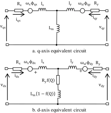
II. MODEL OF T HE LINEAR INDUCT ION MOT OR The (q) axis equivalent circuit of the LIM is identical to the (q) axis equivalent circuit of the rotary induction motor (RIM), i.e. the parameters do not vary with the end effects. However, the (d) axis entry secondary currents affect the air gap flux by decreasing (dy). Therefore, the (d) axis equivalent circuit of the RIM cannot be used in the LIM analysis when the end effects are considered.
From the equivalent circuit of the LIM (Fig.1), the primary and secondary voltages equation in a synchronous reference system aligned with the secondary flux are given by [2]-[10]:
( ) dx
dx x dx y dx dy x qx
d
v R i R Q i i
dt
(4)
Approaches of Vector Control of a Linear
Induction Motor Considering End Effects
qx
qx x qx x dx
d
v R i
dt
(5)
dy 0dy y dy y dx dy
d
v R i R Q i i
dt
(6)
0
qy y qy sl dy
v R i
(7)Where:
( ) ( )
dx L Q ix dx L Q im dy
(8)qx L ix qx L im qy
(9)( ) ( )
dy L Q iy dy L Q im dx
(10)0
qy L iy qy L im qx
(11)While referring to the preceding equations, the primary and secondary currents are given by:
2( ) ( )
( ) ( ) ( )
y dx m dy
dx
y x m
L Q L Q
i
L Q L Q L Q
(12)
2
y qx m qy qx
y x m
L L
i
L L L
(13)
2( ) ( )
( ) ( ) ( )
x dy m dx
dy
y x m
L Q L Q
i
L Q L Q L Q
(14)
2
x qy m qx qy
y x m
L L
i
L L L
(15)
From (7) and (11) the slip frequency is obtained as followed:
1
y qy m
sl qx
dy y dy
R i L
i T
(16)
The slip frequency equation sl is the same as that of the conventional induction motor. The main difference is the characteristic dy.
a. q-axis equivalent circuit
b. d-axis equivalent circuit
Fig. 1. dq-equivalent circuit of the LIM with end effects From (6) and (10), we obtained:
1
y m y
dy dx
m y y
R L L f Q
i
s L L f Q R f Q
(17)
The thrust force is given by:
3 2
e dx qx qx dx
F p
i
i
(18)
After a long manipulation of the equation (18), we obtain:
2 ( )
3
2 1
y m
e dy qx dx qx
y m y
l f Q
L Q
F p i i i
L L f Q L f Q
(19)
The secondary self inductance Ly ly Lm Lm, because the leakage inductancely Lm. In this case, the thrust force Fe does not directly depend on Q. For that, the dependence of
Fe to the speed appears not to be as significant as dy is kept
constant. Thereafter, it will be shown, by simulation, that the dependence of dy to Q is large. Therefore, the thrust force Fe
becomes:
21 2
3
2 1
y
e dy qx dx qx e e
y
l f Q
F p i i i F F
L f Q
(20)
Starting from the preceding equation, the thrust force is not proportional to iqx, due to the existence of the second term in (19) which is produced by the eddy current loss. The second term always has the opposite sign, thus is called „dynamic braking force‟ [5]. In an extreme case such that emergency stop is necessary; the dynamic braking force may be used to assist the motor to stop. But, the dynamic braking force should be compensated to achieve a linear relationship between Fe and iqx.
III. ORIENT ED VECT OR CONTROL WITH MINIMIZATION OF END
EFFECT S
In conventional vector control (without minimization), the end effects give rise to a variation of the primary currents idx
and iqx, therefore by increase of losses in this type of actuator.
To develop an order with minimization of end effects, summons us brought to impose a variable secondary flux dy
according to the operating conditions. The value of this flux is calculated by minimization the losses in this type of motor.
For the steady state, equation (4)-(7) can be transform to (21)-(24)
dx x dx y dx dy x qx
v R i R f Q i i (21)
qx
qx x qx x dx
d
v R i
dt
(22)
0dy y dy y dx dy
v R i R f Q i i (23)
0
qy y qy sl dy
v R i
(24)A. Assessment of the losses
Iron losses are given by the following expression:
2Fe y dx dy
P R Q i i (25)
iqy
Ry
Rx
vqx vqy
ωxϕqx lx ly ωslϕqy
Lm
iqx
+ +
idx idy
Ry
Rx
vdx vdy
ωxϕdx lx ly ωslϕdy
Lm 1 − f Q
Primary copper losses are given by:
2 2
cx x dx qx
P R i i (26) Secondary copper losses are expressed by the following equation:
2 2
cy y dy qy
P R i i (27)
Total losses in a linear induction motor are obtained starting from the equations (25)-(27):
t Fe cx cy
PP P P (28)
The end effects cause a variation of the primary currents; therefore we calculated the total losses according to these currents. We expressed the secondary currents according to the primary current in the following equations:
( )
1 ( )
dy dx
f Q
i i
f Q
(29)
m
qy qx
r
L
i i
L
(30)
From (25)-(30), total losses are given by [11]:
2 2
t d ds q qs
PR i R i (31)
Where:
( )
1 ( )
d x y
f Q
R R R
f Q
(32)
2
m
q x y
y
L
R R R
L
(33)
We note that y 2dx f (Q)
R i
1 f (Q) represents the losses due to the
ends effects. Primary current idx can be expressed according to
dx
as follows:
1 ( )
( )
dx dy
m r
f Q i
L L f Q
(34)
The force is expressed by:
3 3 3
2 2 2
m
e dy qy qy dy dy qy dy qx
y
L
F p i i p i p i
L
(35) From (32)-(33), it follows,
2 2 2
2
2
2 2
2
1 ( 2 1
( ) 3
y e
t d y q
m y m y
e y
y
L F
f Q
P R R
L L f Q p L
F
A B
(36)
Where:
2
1 ( )
( )
d
m y
f Q
A R
L L f Q
(37)
2 2 1 3
y q
m
L
B R
p L
(38)
If we want to gain the minimum Pt (minimum end effects),
then
2 3
2 2 0
t e
y
y y
P F
A B
(39)
As a consequence
* 4
y e
y
B F A v
(40)
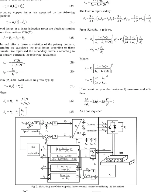
Fig. 2. Block diagram of the proposed vector control scheme considering the end effects
ϕdy∗
icx
ϕdy
Speed controller
iax ibx
iqx∗
3 2P
π τ
Lm(Q)
Ly−Lmf Q ϕdy
∗
iax∗
ibx∗
icx∗
Ry Lm−Lyf Q
s Lm−Lyf Q +Ry 1+f Q
ϕdy
π τ θx
θx
iax
ibx
iqs
iqx
idx
LIM Ec
vax
vbx
vcx
PI
PI
IP Current
controller
Fe
Fe
idx∗
vy∗
vy
vy
ωsl ωy
ωx
dq abc dq
abc
Fe∗
RyLm
Ly
iqx
ϕdy iqse ly2
Ly
f Q 1−f Q
idxiqx
ϕdy flux
estimation
From (40), the secondary magnetic flux * y
corresponding to minimum end effects is determined by force Fe and speed vy.
B. Simulation results
The type of test‟s machine that is considered in this work is linear induction motor with simple primary. Its primary is three phase connected in star. It is characterized by the parameters presented in table I. The bloc diagram of the proposed vector control considering the end effect is given by Fig. 2. The validity of this control approach, elaborated to regulate the secondary speed, is realized by numeric simulation using the Simulink interface of the Matlab environment.
IV. SECONDARY FLUX ORIENT ED VECT OR CONT ROL WIT H
COMPENSAT ION OF END EFFECT S
In a LIM, the end effects are expressed by both the generation and the disappearance of the field that create the eddy current in the reaction rail. The air gap flux is more affected by the eddy current. For this raison, the linkage flux ϕ is separate in two portions: the first is independent of the end effects ( dy1 0.7424Wb ), while the second describes the linkage flux that is due to the end effects (dy2).
1 2
dy dy dy
(41)A. Basic idea for the compensation
The LIM‟s primary currents are separable into two portions. The first portion is the current in a conventional machine and the secondary portion is a current due to the LIM‟s end effects. Based on equation (17), the primary current idx is [12]:
For no load, secondary flux is fixed at its nominal value (
dy 0.7424Wb
) to have a good fluxing of the machine. For a given load, flux varies according to this load and speed forced so as to have a minimal end effects.
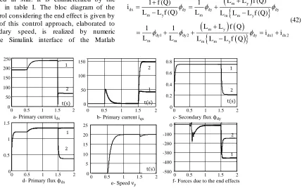
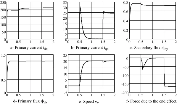
The results of simulation show that the influence of the end effects on idx current is more significant than that on iqx
current. Indeed, for a speed of 20 m/s, the variation of idx is
about 48A whereas the variation of iqx is approximately 5A.
At no load, the results obtained by the two methods are identical. This idea enables us to have a good fluxing of the machine. At load, the curves representing the currents and flux are different. Indeed, idx current is equal to 236.3A for
conventional method and equal to 66.12A for the proposed method.
m y
dx dy dy dy
m y m m m y
m y
dy1 dy2 dy dx1 dx 2
m m m m y
L L f (Q)
1 f (Q) 1
i
L L f (Q) L L L L f (Q)
L L f Q
1 1
i i
L L L L L f Q
(42)
Where:
1 1
1
dx dy
m
i
L
(43)
2 2
1 m y
dx dy dy
m m m y
L L f Q
i
L L L L f Q
(44)
Based on equation (18), the primary current iqx is:
2 2 1
3 ( )
1 ( )
e qx
y
dy dx
y
F i
P l f Q
i
L f Q
(45)
After a long manipulation of the equation (45), we obtained:
1
2
2
1 2
2 1 3
2 1 3
e qx
dy
dy dx
e
dy dy dy dy dy dx qx qx
F i
P
Ai F
P Ai
i i
(46) Fig. 3. Response of velocity control with end effects (1: without minimization; 2: with minimization)
c- Secondary flux ϕdy
0 0.5 1 1.5 2 0
0.2 0.4 0.6 0.8
t(s)
1
2
b- Primary current iqx
0 0.5 1 1.5 2 0
50 100 150
t(s)
2
1
a- Primary current idx
0 0.5 1 1.5 2 0
50 100 150 200 250
t(s)
2 1
f- Forces due to the end effects
0 0.5 1 1.5 2 -500
-400 -300 -200 -100 0
2
1
e- Speed vy
0 0.5 1 1.5 2 0
5 10 15 20 25
t(s)
d- Primary flux ϕdx
0 0.5 1 1.5 2 0
0.5 1 1.5
1
Where:
2
( )
1 ( )
y y
l f Q
A
L f Q
(47)
1
1 2 1 3
e qx
dy
F i
P
(48)
2
2
2 2 1
3
dy dx
qx e
dy dy dy dy dy dx
Ai
i F
p Ai
(49)
B. Neural Network
The (d, q) currents dependent of the end effects (ids2 and
iqs2) are related to dy2. To calculate dy2 in real time, a
neuronal model is used. The inputs of the Neural Network (NN) are the secondary speed vy and the load force Fl, the
output of the NN is the variation of dy due to the end effects. The connective weights and biases of the NN are adjusted by a data base to produce dy2. The neural network understands
three layers; - Input layer:
In the input layer, the input vector of the NN is the secondary speed and the load force:
1, 2k k
k k i k
y x
k
f y y
(50)
V.PRIMARY FLUX ORIENT ED VECT OR CONT ROL The control strategies developed previously are very sensitive to the secondary parameters variation. To cure this insufficiency, another approach of vector control based on the primary flux oriented is developed.
Where:
1 y( )
x v t , x2F tl( ) (51)
- Hidden layer:
1 1, ,1 i
i ik k i
k
i i i y
y W
i m
f y
e
(52)
Where Wik are the connectives weights between the input and
hidden layers; k are the threshold values for the units in the hidden layer; fi is the activation function, which is a sigmoid
function. - Output layer:
1j ij i k
j j j j
y W
j
f y y
(53)
Where Wji are the connective weights between the hidden and
the output layers; θk dy2
C.Simulation results
The strategy of control with compensation consists in acting on different regulators to impose idx1 and iqx1 such as
variables of control.
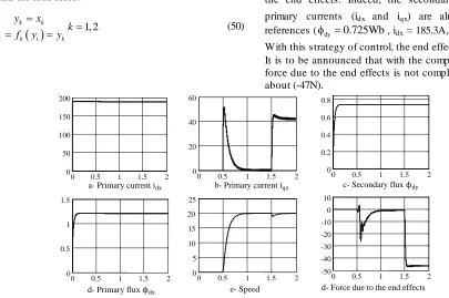
Fig. 4 shows the simulation results with compensation of the end effects. Indeed, the secondary flux dy and the primary currents (idx and iqx) are almost equal to their
references ( dy 0.725Wb, idx = 185.3A, and iqx = 41.3A).
With this strategy of control, the end effects are compensated. It is to be announced that with the compensation method, the force due to the end effects is not completely neutralized. It is about (-47N).
The eddy current loss of the secondary conductor must be to describe by a parallel resistor, same as the core loss [4]. However, in Duncan‟s model, the eddy current loss is described by a series resistor.
In this phase study, we neglected the eddy current loss (Ry.f(Q)). However, the inclusion of the loss branch increases
the complexity of the equation greatly, whilst the presence or absence of the loss branch does not make a significant difference in the current dynamics unless SLIM is moving at a very high speed [4].
Fig. 4. Results obtained with compensation of the end effects a- Primary current idx b- Primary current iqx
d- Primary flux ϕdx
c- Secondary flux ϕdy
d- Force due to the end effects
0 0.5 1 1.5 2 -50
-40 -30 -20 -10 0 10
0 0.5 1 1.5 2 0
0.2 0.4 0.6 0.8
0 0.5 1 1.5 2 0
20 40 60
e- Speed
0 0.5 1 1.5 2 0
5 10 15 20 25 0 0.5 1 1.5 2 0
50 100 150 200
0 0.5 1 1.5 2 0
The idea remains unchanged; it is a question of acting in instantaneous and independent manner on the phase and the amplitude of the primary voltage, so as to regulate current iqx
without modifying flux dx.
A. Mathematical equations of the machine
The primary and secondary voltages equations are given by [4], [13]:
dx dx x dx
d
v R i
dt
(54)
qx x qx x dx
v R i
(55)vdy R iy dy d dy sl qy 0 dt
(56)
0
qy qy y qy sl dy
d
v R i
dt
(57)
The dq-axis flux linkages of primary and secondary are given by:
( ) ( )
dx L Q ix dx L Q im dy
(58)( ) ( )
qx L Q ix qx L Q im qy
(59)( ) ( )
dy L Q iy dy L Q im dx
(60)( ) ( )
qy L Q iy qy L Q im qx
(61)These two functions (66) and (67) show significant sensitivity to the variations of primary resistance. To note that because of the end effects, the control of primary resistance is easier with the evolution of secondary resistance.
While referring to the preceding equations, the primary and secondary currents are given by:
2( ) ( )
( ) ( ) ( )
y dx m dy
dx
y x m
L Q L Q
i
L Q L Q L Q
(62)
2( ) ( )
( ) ( )
y qx m qy
qx
y x m
L Q L Q
i
L Q L Q L Q
(63)
2( ) ( )
( ) ( ) ( )
x dy m dx
dy
y x m
L Q L Q
i
L Q L Q L Q
(64)
2( ) ( )
( ) ( ) ( )
x qy m qx
qy
y x m
L Q L Q
i
L Q L Q L Q
(65)
The primary equations (54) and (55) constitute the estimators homologous with those of the control based on secondary flux oriented.
Indeed, the speed vx results directly from the following
relation:
qx x qx e
x e
x
v R i
v
(66)
And the flux is expressed directly starting from the following formula:
0
t e
x vdx R ix dx dt
(67)We show that there is a similar property in the case of primary flux oriented. The secondary equations (56) and (57) of the model are initially transformed to reveal the secondary sizes. The secondary currents result from the expression of primary flux.
x x dx dy
m
L Q i i
L Q
(68)
x
qy qx
m
L Q
i i
L Q
(69)
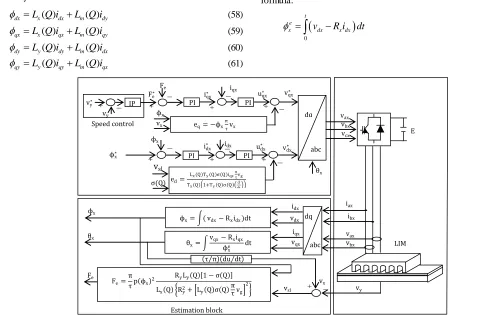
Fig. 5. Block diagram of the primary flux oriented vector control
LIM
Fe
iax ibx θx
vqx
E
ϕx
vax vbx vdx
idx iqx
Estimation block
vy dq
ϕx∗
ϕx Speed control
IP Fe vy∗
vy
Fe∗
eq= −ϕxπτvx iqx∗ PI
idx∗ PI
iqx u qx ∗ PI
vqx∗
udx∗
PI vdx
∗ idx
ed=
Lx Q Ty Q σ Q iqxπτvg
Tx Q 1+Ty Q σ Q dtd ϕx
vx
vsl
σ(Q)
θx dq
abc vax vbx vcx
abc ϕx= ( vdx− Rxidx)dt
θx=
vqx− Rxiqx ϕxe dt τ π du dt
vsl
vx Fe=
π τp ϕx2
RyLy Q 1 − σ Q Lx Q Ry2+ Ly Q σ Q πτ vg
Under these conditions, secondary fluxes are written:
y x y
dy x m dx
m m
L Q L Q L Q
L Q i
L Q L Q
(70)
x
yqy m qx
m
L Q L Q
L Q i
L Q
(71)
What carries out the new system of secondary equations, are:
0 1 y( ) x x 1 y dx
y x sl dx
d d
T Q L Q T Q Q i
dt dt
T Q L Q Q i
(72)
0
1 1
x x dx sl
y x qx
y
Q L Q i v
d
T Q Q L Q i
T Q dt
(73)
By combining these two last equations to eliminate idx, we
express iqx according to speed vsl, it comes:
2
21
1
qx
y x
sl
x y y sl
i
T Q Q
v d
L Q T Q Q T Q Q v
dt
(74) The formula giving the force becomes:
2
2 2
3
2 .
3
2 1
1
e x qx x
y x
sl
x y y sl
F p i p
T Q Q
v d
L Q T Q Q T Q Q v
dt
(75) In steady state, the derivative becomes null and, after having expressed Ty (Q), the expression (75) becomes:
2
2 2
1 3
2
y y
e x
sl
x y
s y
l
R L Q Q
F p v
L Q R L Q Q v
(76)
In the equation (54), we express idx starting from the
expression (72). It comes:
1
1
1
y x
dx x
x
y
x y
qx sl
x y
d T Q
R dt
v
d L Q
Q T Q dt
R Q T Q v
d i
d dt
Q T Q dt
(77)
This last equation associated with the expression (55) models the electric part seems two mono-variable processes coupled by the variables of disturbance ed and eq such as:
2 2 1
1
x y x y x
x y dx d
d d
T Q T Q Q T Q T Q
dt dt
d
T Q Q T Q v e
dt
(78)
x qx qx q
R i v e (79)
Where
1
q x y
x y qx
d
l
sl y
s
x
e v v
Q L Q T Q i v
e
d
T Q Q T Q
dt
(80)
B. Simulation results
For this control, the adjustment structure is given by fig. 5. For the vector control with primary flux oriented, fig. 6, primary flux dx remains constant and equal to 1.242Wb whereas secondary flux dy decreases according to speed.
Current idx undergoes a weaker variation compared to the first
strategy. The primary current iqx does not undergo any
VI. CONCLUSION
The minimization and compensation of the end effects in a LIM constitutes the principal theme in this paper. For that, an approach of modeling is developed to hold account the end effects which characterize this type of machine. The minimization idea consists in forcing secondary flux (dy) so
as to have minimal losses. This strategy shows that idx current decreases whereas iqx current increases. These change lead to good results. The strategy of compensation consists in estimating the primary flux variation by a Neural Network. This flux is used to determine the secondary currents dependent of the end effects. The compensation is ensured by action on the different regulators. The obtained simulation results show that the end effects can be compensated. The control strategies developed previously are very sensitive to the secondary parameters variation. To cure this insufficiency, another approach of vector control based on the primary flux oriented is developed.
REFERENCES
[1] GIERAS, J. F., Linear Induction Drives, Oxford, U. K. Clarendon Press, 1994.
[2] BHAT IA, R. P. and SNIDER, D. R., T hrust Expressions for Induction Motors with T hin Conducting Secondaries, IEEE Trans. Magn., Vol. 26,
No. 2, pp. 1101-1106, March 1990.
[3] GIERAS, J. F., DAWSON, G. E. and EAST HAM, A. R., A new longitudinal end effect factor for linear induction motors, IEEE Transaction on Energy Conversion, Vol. EC-2, No. 1, pp. 152-159, March 1987.
[4] KAN, G. and NAM, K., Field-oriented control scheme for linear induction motor with the end effect, IEE, Proc. Electr. Power Appl. Vol.
152, No. 6, pp. 1565-1572, Novem ber 2005.
[5] SUNG, J. H. and NAM, K., A New Approach to Vector Control for Linear Induction Motor Considering End Effects, IEEE IAS annual
m eeting, Phoenix, Arizona, pp. 2284 -2289, October 3-7, 1999.
[6] DUNCAN, J. and ENG, C., Linear induction motor-equivalent circuit model, IEE Proc., Electr. Power Appl. Vol. 130, No. 1, pp. 51 -57,
January 1983.
[7] DA SILVA, E. F., DOS SANT OS, E. B., MACHADO, P. C. M. and DE OLIVEIRA, M. A. A., Dynamic Model for Linear Induction Motors,
IEEE ICIT Conference, Maribor, Slovenia, pp. 478 -482, 2003.
[8] DA SILVA, E. F., DOS SANT OS, E. B., MACHADO, P. C. M. and DE OLIVEIRA, M. A. A., Vector Control for Linear Induction Motor, IEEE
ICIT Conference, Maribor, Slovenia, pp. 518 -523, 2003.
[9] DA SILVA, E. F., DOS SANT OS, E. B. and DE NERYS, J. W. L., Field oriented Control for Linear Induction Motor T aking into Account End effects, IEEE International workshop on Advanced Motion,
Kawasaki, Japan, pp. 684-694, 2004.
[10] HAJJI, M., NASR KHOIDJA, M. A. and BEN SALAH, B., Direct thrust control of a Linear Induction Motor with end effects, International Review of Electrical Engineering, Vol. 4, No. 4, pp. 539 -546, July-August 2009.
[11] HAJJI, M., NASR KHOIDJA,M. A., BARHOUMI, E. M., and BEN SALAH, B., “ Vector Control for Linear Induction Machine with Minimization of the end effects” The First International Conference on Renewable Energy and Vehicular Technology, REVET, March 26
-28,2012, Ham m am et-Tunisia.
[12] HAJJI, M., NASR KHOIDJA, M. A. and BEN SALAH, B., Vector control for Linear Induction Motor with Compensation of the end effect, International Review on Modeling and Sim ulation, Code ISSN
1974-9821, Vol. 4, No. 1, pp. 20-26, February 2010.
[13] HAJJI, M., NASR KHOIDJA, M. A. and BEN SALAH, B., “ Vector Control for Linear Induction Machine Considering End Effects” the 12th International Conference on Sciences and Techniques of Automatic Control and Computer Engineering, Decem ber 18 -20, 2011, Sousse, Tunisia.
APPENDIX Fig. 6. Results obtained by the secondary flux oriented vector control
0 0.5 1 1.5 2
0 50 100 150 200 250
0 0.5 1 1.5 2
0 5 10 15 20 25 30 35
0 0.5 1 1.5 2
0 0.2 0.4 0.6 0.8
a- Primary current idx b- Primary current iqx c- Secondary flux ϕdy
0 0.5 1 1.5 2
0 0.5 1 1.5
0 0.5 1 1.5 2
-5 0 5 10 15 20 25
0 0.5 1 1.5 2
-200 -150 -100 -50 0
d- Primary flux ϕdx e- Speed vy f- Force due to the end effects
T ABLEI
DESIGN DATA OF THE P ROP OSED SLIM
Symbol Quantity Value
τ Pole pitch 250 mm
p Number of poles 6 Resistance of primary per
phase
0.0968Ω Resistance of secondary per
phase