On Classification Approaches for Misbehavior Detection in Wireless Sensor Networks

On Classification Approaches for Misbehavior

Detection in Wireless Sensor Networks

Matthias Becker

Martin Drozda

Sven Schaust

Sebastian Bohlmann

Helena Szczerbicka

Welfengarten 1, 30167 Hannover, Germany

Email:{xmb, drozda, svs, bohlmann, hsz}@sim.uni-hannover.de

Abstract— Adding security mechanisms to computer and communication systems without degrading their perfor-mance is a difficult task. This holds especially for wireless sensor networks, which due to their design are especially vulnerable to intrusion or attack. It is therefore important to find security mechanisms which deal with the limited resources of such systems in terms of energy consumption, computational capabilities and memory requirements.

In this document we discuss and evaluate several learning algorithms according to their suitability for intrusion and attack detection. Learning algorithms subject to evaluation include bio-inspired approaches such as Artificial Immune Systems or Neural Networks, and classical such as Decision Trees, Bayes classifier, Support Vector Machines,k_-Nearest Neighbors and others. We conclude that, in our setup, the more simplistic approaches such as Decision Trees or Bayes classifier offer a reasonable performance. The performance was, however, found to be significantly dependent on the feature representation.

Index Terms— Attack, Intrusion and Anomaly Detection; Wireless Sensor Networks; Artificial Immune Systems; Ma-chine Learning; Bio-Inspired Approach.

I. INTRODUCTION

A Wireless Sensor Network (WSN) consists of small battery powered wireless devices (sensors) that are ca-pable of monitoring environmental conditions such as humidity, temperature, noise, etc. Sensor networks do not have a fixed infrastructure but form an ad hoc topology using wireless communication channels. In many scenar-ios, it is expected that environmental data, collected by a sensor network, gets evaluated remotely. This implies a necessity of a gateway (collection) wireless device that is directly connected to an external network, possibly to the Internet.

After sensors get deployed in the monitored area, the access to them can be difficult. For example, a sensor network, with the goal to monitor conditions in the sewer system of a large city, might be inaccessible for mainte-nance, software updates or battery exchange. Therefore, a special focus has been put on designing energy efficient protocols at all layers of the OSI (Open Systems Intercon-nection) protocol stack; see [1] for a thorough review of protocols for sensor networks. Additionally to addressing

This paper is based on “Performance of Security Mechanisms in Wireless Ad Hoc Networks,” by M. Becker, M. Drozda, and S. Schaust, which appeared in the Proceedings of the Workshop on Security and High Performance Computing Systems, Nicosia, Cyprus, 2008

energy constraints, these protocols should impose a high degree of robustness in order to minimize the need for human intervention.

Since sensor networks are expected to become an important part of technical infrastructure, their failure can lead to substantial decrease in services or even cause financial losses. Sensor networks can also be subjected to various forms of intrusions and attacks. The motivation for attacking a sensor networks could be, for example, to gain an undeserved and exclusive access to the collected data. There has been a multitude of attacks described in the literature: probabilistic data packet dropping, topol-ogy manipulation, routing table manipulation, prioritized data and control packet forwarding, identity falsification, medium access selfishness etc. We refer the reader to [2] for a more complete list of attacks and intrusions.

The protection system of a sensor networks usually relies on the following two mechanisms: (i) authentica-tion and secure protocols and (ii) intrusion and attack (misbehavior) detection. As the experience from the In-ternet shows, the weaknesses in authentication and secure protocols are frequently exploited. These protocols alone are in general considered being insufficient to provide the necessary level of protection [3]. Therefore, there has been a lot of effort invested in providing networks with means for a timely detection of an attack or intrusion. Such detection is often based on methods and algorithms known from the field of machine learning [4].

Our goal was therefore to investigate the feasibility of different learning and classification algorithms for detection of misbehavior in sensor networks. The choice of learning algorithms is based upon the fact that mis-behavior is rather unforeseeable and thus an intelligent approach is necessary in order to respond to unknown misbehavior (caused by new forms of attacks).

information available about the shape and complexity of the underlying space. We could however show that the space is severely impacted by the choice and complexity of the chosen communications protocols.

Even though AIS based approaches look promising, it was an open question whether AIS fit well the task of misbehavior detection. We therefore wanted to contrast AIS with other approaches such as Neural Network, Decision Trees, Bayes classifiers etc. Our main goal was to evaluate these different learning algorithms in several experiments using an identical scenario.

This document is structured as follows. First, we give a short overview on protocols in WSN and of our ap-proach to misbehavior detection in sensor networks. In Section IV we give a brief overview of the different kinds of classification algorithms which were employed. In Section V, an outline of the experimental setup is presented. In Section VI we present the features used in classification. In Section VII we present the results and, finally, in Section VIII we conclude.

II. PROTOCOLS FORWSN

Data exchange in a point-to-point (uni-cast) scenario usually proceeds as follows: a user initiated data exchange leads to a route query at the network layer of the OSI stack. A routing protocol at that layer attempts to find a route to the data exchange destination. This request may result in a path of non-unit length. This means that a data packet in order to reach the destination has to rely on successive forwarding by intermediate nodes on the path. An example of an on-demand routing protocol often used in sensor networks is DSR (Dynamic source routing) [12]. Route search in this protocol is started only when a route to a destination is needed. This is done by flooding the network with RREQ1 _{control packets. The destination}

node or an intermediate node that knows a route to the destination will reply with a RREP control packet. This RREP follows the route back to the source node and updates routing tables at each node that it traverses. A RERR packet is sent to the connection originator when a node finds out that the next node on the forwarding path is not replaying.

At the MAC (Medium access control) sublayer of the OSI protocol stack, the medium reservation is often contention based. In order to transmit a data packet, the IEEE 802.11 MAC protocol uses carrier sensing with an RTS-CTS-DATA-ACK handshake.2 _{Should the medium}

not be available or the handshake fails, an exponential back-off algorithm is used. This is combined with a mechanism that makes it easier for neighboring nodes to estimate transmission durations. This is done by exchange of duration values and their subsequent storing in a data structure known as Network Allocation Vector (NAV).

The 802.11 protocol was, however, mainly designed for networks with high data rates (above 1Mbit/s) and not

1_{RREQ = Route Request, RREP = Route Reply, RERR = Route Error.} 2_{RTS = Ready to send, CTS = Clear to send, ACK =}

Acknowledg-ment.

for energy restricted sensor networks. There has been a continuing effort to propose medium access protocols that would better fit the needs of sensor networks. Examples of such specialized medium access protocols are the IEEE 802.15.4 and S-MAC protocols [13].

III. MISBEHAVIOR DETECTION INWSN Our approach to misbehavior detection in WSN re-lies on the ability of a given wireless device (node) to efficiently analyze its own states and events as well as all observable events and states in its physical neighbor-hood. A neighboring node is said to be in the physical neighborhood of a node, if this given node is able to overhear the traffic of the neighboring node. All states and events are evaluated and averaged over a sliding time window. Each node in the network runs an instance of the learning algorithm. This implies that each node is able to detect whether one of his neighbors is likely to misbehave. Our approach currently does not include any exchange of detection information, there is no collective evaluation of misbehavior and it does not support any actions that would be able to suppress or eliminate the consequences of a misbehavior on a sensor network.

We would like to note that overhearing the traffic in the neighborhood assumes that the given node is able to operate in the so-calledpromiscuous mode. Operation in promiscuous mode is rather energy inefficient since the node has to stay on all the time. There have been several approaches aimed at energy preservation at nodes. One of the approaches suggests, each node should publish its listen-sleep schedule. An example of a protocol utilizing a listen-sleep schedule is the S-MAC protocol [13]. This protocol, though, being more energy efficient than for example the IEEE 802.11 protocol, severely limits the ability of a node to observe events and states in its physical neighborhood. Our goal was however not to investigate quality and feasibility of various features for classification but rather to give an insight about the performance of several learning and classification algo-rithms, if used in the context of misbehavior detection in sensor networks. Our goal was therefore to elucidate the relationship between learning algorithms and their performance on one side, and between their performance and suitability for sensor networks on the other side.

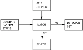
DETECTOR SET MATCH NO

YES

REJECT STRINGS SELF

STRING RANDOM GENERATE

Figure 1. Detector generation by random-generate-and-test process. Only strings that do not match anything self become detectors.

MATCH STRINGS NEW

YES DETECTOR

SET

DETECTED NON−SELF

Figure 2. Recognizing non-self is done by matching detectors with suspected non-self strings.

IV. CLASSIFICATIONAPPROACHES

In our initial studies we used AIS [10], [11], [14] as it seemed to be a promising tool for misbehavior detection. However AIS have some drawbacks and weaknesses that need to be studied with respect to the proposed application area, i.e. resource limited sensor networks. Therefore we undertook an initial comparative study with Neural Networks [15] and subsequently evaluated several major classification algorithms [16].

A. Summary of Classification Algorithms

For Decision Trees, k-nearest neighbors, Chi-square Automatic Interaction Detectors (CHAID), Neural Net-works and naive Bayes classifiers we used the implemen-tations given in Yale [17]. For the AIS we used our own implementation; details about the AIS implementation can be found in [10], [14].

1) Artificial Immune Systems: Inspired by the Human Immune System, AIS have already been considered for misbehavior detection in communication networks, and especially in flexible environments such as ad hoc and sensor networks. The AIS in our setup, requires two phases: learning phase and detection phase. During the learning phase, a so called self-set, which represents the expected behavior, serves as a basis for computing a set of anomaly detectors. This process is in our setup performed using anegative selection mechanism. In negative selec-tion, candidate detectors are produced randomly and then compared with the self-set. Should a candidate detector match some element in the self-set, it gets removed. Candidate detectors that do not match anything in the self set are included into the detector set. This process is depicted in Figure 1.

The detection (or testing) phase uses the set of detectors in order to detect anomaly. Therefore behavior patterns (antigens) of features, computed from the network traffic

observable in a node’s neighborhood, have to be created for an observed time window. A pattern is matched against the complete detector set and if a positive match is found an observed anomaly is reported for the specific time window. This process is depicted in Figure 2. Both Figure 1 and 2 assume that the bit-string representation is used. Other widely investigated representation approach includes real-value vectors [18].

The learning mechanism used in AIS is adopted from the process of T-cell maturation and selection in the thymus. The role of detectors is to detect non-self anti-gens. A popular algorithm for matching detectors and antigens, if represented as bit-strings, is ther-contiguous bits matching rule. Two bit-strings of equal length match under this matching rule, if there exists a substring of lengthrat positionp in each of them, which is identical in both bit-strings.

The negative selection process is known to perform unfavorably in highly complex spaces. It was initially analyzed in [19] where it was shown that the number of candidate detectors grows, in general, exponentially with the size of the self set. Recently, it was shown by Timmis et al. that the negative selection approach is NP-complete [20]. A good review of other approaches motivated on the Human Immune System can be found in [5], [21].

2) Neural Networks: Neural Networks using back-propagation as learning mechanism are a well known approach, therefore only a brief review of the algorithm is given (see [22] for more details).

Neural Networks typically consist of several neuron layers, namely an input layer, one ore more hidden layers and an output layer. Input neurons learn a function from an input vector to an output vector. During the learning phase, input vectors are presented to the network and an output vector is calculated. Depending on the resulting output vector (correct or not), the weights in the Neural Network are changed using a back-propagation algorithm in order to achieve the correct output. This procedure is repeated until the correct output is calculated for all input vectors (with someǫ error possible).

In order to train a Neural Network the available data is divided into a training and a test set. During the learning phase the training set is used to train the network. The test set is used in order to evaluate the network’s ability forpredictionof unknown input vectors.

During the learning phase it is necessary to avoid the problem of over-fitting, causing the Neural Network to create a specific output vector regardless from the input given (see [23]).

ex-periments, namelySVM with particle swarm optimization (SVM-PS, [24]) andSVM with evolutionary optimization (SVM-Evo, [25]). Both use a binary classifier with a hyperplane to separate class members from non-members in a high dimensional space and a radial kernel type.

For the SVM-PS a population size of100with a maxi-mum of500evaluations has been selected. The local and global knowledge of the best individuals are combined with the same level of relevance. In our experiment a start setup of 10 individuals was chosen for the SVM-Evo. Mutation is enabled with a Gaussian distribution. For selection a tournament mode with a fraction of0.75 is used. The best individual solution survives under all circumstances.

4) Decision trees [26]: In general, Decision Trees are a method to classify data based on conjunctions of features which lead to the specific classification, whereas the classification is represented as a leave in the tree. In our experiments a binary tree representation is used, where every tree node corresponds to an input parameter. The basic criterion is to achieve a decreasing information gain on the path to the leafs. We allowed a maximum tree height of size 10.

5) k-Nearest Neighbors [27]:Thek-Nearest Neighbor algorithm (KNN) classifies input vectors based on a majority vote of its neighbors, assigning the vector to the most common class amongst itsk-Nearest Neighbors. KNN is trained using vectors of ad-dimensional feature space. This feature space is partitioned into regions and labels using a training set. Apoint(vector) in the space is assigned to a class if it is the most frequent class among the k-nearest training samples. During the test phase, the distances of a new vector to all stored vectors are computed and the k closest ones are selected. Then the most common class amongst the k neighbors is chosen and assigned to the new vector. In our experiments the mixed Euclidean distance has been used for calculation of the distances between the vectors.

6) Chi-square Automatic Interaction Detectors [28]– [30]: The CHAID-algorithm described by Anderberg in 1973 is a Decision Tree algorithm using theχ2

attribute relevance test during the tree building process. The test decides whether two variables are dependend or not, thus creating different branches from a parent node. The algorithm uses a tree structure, where every node is allowed to have more than two children in order to keep the tree compact. The growing of the Decision Tree is limited using a pruning mechanism during the tree building process. The same parameter combinations as for the simple Decision Tree are used.

7) Naive Bayes [31]: A naive Bayes classifier is a probabilistic classifier based on the Bayes’ theorem with naive independence assumptions. The Bayes approach assumes that the presence of a particular feature of a class is not related to the presence of any other feature. An advantage of the naive Bayes classifier is that it requires only a small amount of training data to estimate the pa-rameters necessary for classification. For our experiments

an estimated normal distribution as classification model is used.

V. EXPERIMENTSETUP

The sensor network consists of1718nodes with a com-munication radio radius of100m. Nodes are distributed randomly over a square area of 2900m ×2950m using a snapshot of a random waypoint mobility model. This approach was motivated by the results gained from eval-uating the structural robustness of sensor networks [32].

During our experiments we used two packet injection models, namely constant bit rate and Poisson distributed packet injection. Additionally the impact of the network congestion using10and50 connection with data packet sources was considered. Each connection has a differ-ent destination and the distance between sources and sinks was chosen to be approx. 7 hops, so that inter-mediate nodes were shared between some connections. As misbehavior in our scenarios we used probabilistic packet dropping with three levels of dropping proba-bilities (10%,30%,50%). Also ”normal” traffic with no misbehavior was simulated, to ensure that ”self” could be learned by the different learning algorithms from these normal behavior runs.236nodes were setup to misbehave, however, only 10− 15 were forwarding enough data traffic. I.e. there was a small number of nodes that could actively misbehave (drop packets). The reason is, a majority of the236nodes did not lie on any active routing path.

For each packet received or sent in the experiment by a node the following information was captured:

• IP header type (UDP, 802.11, DSR)

• MAC frame type (RTS, CTS, DATA, ACK)

• Current simulation clock

• Local source

• Local destination

• Global source

• Global destination

• Packet size

Glomosim [33] was used as network simulator creating 4-hours of simulated traffic. Each scenario was repeated 20times with independent Glomosim runs (80in total as we had one normal run and three different misbehavior runs). In each run for every node the packet information was collected in28non-overlapping time windows of size 500seconds. For each time window and for every node an antigen was computed representing the current node status. The different measured network features which we used in our experiments are described in the following subsection.

VI. FEATUREEXTRACTION

1) MAC layer ratio:

The ratio of complete MAC layer handshakes be-tween a node si and its successor si+1 on a path

and the RTS packets sent bysitosi+1is computed.

Note if there is no traffic between two nodes this ratio is set to ∞ (a large number). This ratio is averaged over a time period. A complete MAC layer handshake is defined as a completed sequence of the MAC layer packets RTS, CTS, DATA and ACK between the two nodes.

2) Forward ratio DATA:

The ratio of data packets sent fromsi tosi+1 and

then subsequently forwarded tosi+2 is computed.

If there is no traffic between the nodes this ratio is set to∞(again a large number). This computation requires nodesi to be in promiscuous mode. The feature was adapted from the watchdog idea in [34]. 3) Average delay DATA:

The time delay that a data packet spends at node

si+1 before being forwarded to si+2 is measured.

The time delay is observed by si in promiscuous mode. If no traffic is between the two nodes, the delay is set to zero. This measure is averaged over a time period. It is a quantitative extension of the previous measure.

4) Forward ratio RERR:

The same ratio as in2 but computed separately for RERR routing packets.

5) Average delay RERR::

The same ratio as in3 but computed separately for RERR routing packets.

Each computed feature was discretized into a 10-bit signature, where each bit defines a certain value range. All computed bit-strings were then concatenated forming a50-bit string. Each self and non-self pattern (antigen in case of the AIS) has therefore a size of50bits.

Additionally to the five features above, we also em-ployed a statistical evaluation process for feature extrac-tion. We declared for every event type a discrete event counter (14 in total) and tested several combinations of these counters as possible features using clustering tests. The clustering method suggested30possible feature combinations, all representing some ratio. We evaluated the significance of these30 combinations and eventually found six significant features, namely

1) forward ratio(DATA) 2) reaction index(RTS/CTS)

3) completed handshakes(i.e. completed data transfer) 4) routing ratio(percentage of routing packets) 5) ratio of unrouted packets(i.e. percentage of packets

that arrive at a node and do not leave the node) 6) number of completed handshakesa node is involved

in for both directions

The average packet delay which was used in the first experiments was found not to be a significant measure as the misbehavior in our case was packet dropping and not delaying packets. However the approximated standard deviation of the delay as a value based on the

average value seems to be significant. All six features form together a suitable combination to detect packet dropping misbehavior in a running scenario where route discovery has already been performed. As we also wanted to detect possible misbehavior during the startup phase of a sensor network we added the average packet size (average and standard deviation) and the packet delay (average and standard deviation) as features. Note that the last two features ratio of unrouted packets and number of completed handshakes do not create any significant clusters of their own, but have relevance in combination with others.

These ten features were used in our later experiments trying to evaluate the suitability of other learning al-gorithms besides AIS. We again used a time window mechanism (800seconds this time), but instead of using a discretized representation, we used a real value repre-sentation for classification. First experiments showed that it was possible not only to distinguish between normal behavior and misbehavior, but also to distinguish the different levels of misbehavior. Therefore every feature calculated in a time window was linked with a specific error state (0%, 10%, 30%, 50% misbehavior). After processing the data, ten-dimensional input vectors divided into four classes were ready to be used together with a set of standard classification algorithms.

A. Classification Experiments

We performed several different classification experi-ments using the basic and the extended feature set. First we took a closer look on the AIS detection capabilities using the basic feature set and studied the influence of the traffic shape on the performance of the AIS.

Since the basic AIS approach needs a special represen-tation in form of a discretized feature set for the data to be learned, first comparisons with other algorithms had been carried out using such a discretized representation together with the described basic feature set. The results of these experiments were not satisfactory for some of the other approaches. To a great extent this has been caused by the data representation, which was tailored to fit to the matching algorithm being used within the AIS approach. So in a next step, the extended feature set was used for the other algorithms together with a feature representation based on real values forming ten-dimensional input vectors.

Additionally for both experiments with classical algo-rithms we added white Gaussian noise to the normalized measurements in order to verify the algorithms prediction abilities.

VII. RESULTS A. Influence of Traffic Quality on AIS

In this section we take a closer look at the AIS and how the data traffic quality and different levels of misbehavior influence the detection success.

Figure 3. Detection rates and False Positives Rate (FP) in percentage (left) and standard deviation (right) for AIS with CBR and Poisson traffic.

traffic, both for three levels of misbehavior (10,30 and 50%). Dealing with CBR seems to be more difficult than with Poisson traffic, especially when the misbehavior level is low in the network (10%). The overall results are reasonable since if little misbehavior (packet dropping in this case) is present, it is hardly distinguishable from normal packet loss that frequently occurs during normal operation of an ad hoc sensor network due to packet collisions and environmental conditions.

Using Poisson data traffic shows more variation for each observed time window, caused by a bigger vari-ance in feature measurements. As a result the learning algorithm trained on a normal traffic with much smaller variation shows better results, as can be seen on the detection rate and the rate of false positives. This is in contrast to the CBR traffic, which produces data with lesser variation. This means, variation naturally occurring in the detection phase gets classified as bad behavior. We conclude, it is desirable to test misbehavior detection algorithms in scenarios where significant misbehavior is present in order to distinguish it from naturally occurring failures.

B. Comparison of AIS with Other Learning Algorithms

The following experiments deal with the feasibility of other learning algorithms for misbehavior detection in our scenario. For the sake of comparability we used the basic feature set with a discretized input data representation and compared the results to the AIS approach. For result validation we used a split-up of three sets, combining two of them for learning and one for testing. Three different combinations of sets were used for the experiments. For each classification algorithm all learning tasks were performed. We only used the highest possible misbehavior level and the misbehavior free traffic for classification. Nonetheless almost all classification algorithms fail in these experiments, with a majority of the test data being classified as ambiguous. As the classification algorithms were not able to separate the two groups based on the given information, a new group named undefined was introduced, having all undecidable input vectors as members. The state space of this experiment is 105

, as

each feature was discretized into a 10-bit string. Only 62diverse feature combinations over all simulation runs were found using this kind of representation. Of these many were used several times. After relabeling the vectors to the three groups (norm, misbehavior, undefined) only traffic samples including all three activity groups were used for classification. We also conducted the experiment with different noise levels and observed that a noise level≤5%does not significantly influence the prediction process of the classical learning algorithms (the figures are not included). For the AIS equivalent data input the results in Figure 4 in comparison to Figure 5 show, that the performance of the classical algorithms is highly dependent on the chosen input representation.

C. Performance of other learning algorithms using the extended feature set and standard data representation

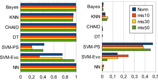
Since the other algorithms seemed to perform unfavor-ably with the classification based on the data representa-tion designed for AIS, we repeated the experiment, using real valued vectors as a representation together with the extended feature set. As indicated above, our goal was to classify a given vector as either normal or representing one of the three misbehavior levels. I.e. we used not only a good / bad classification but we distinguished among all four levels, namely normal (or0%),10%,30%

Figure 5. Prediction rates (left) and standard deviation (right) of the classification algorithms for four misbehavior levels (0,10,30,50%).

and 50% misbehavior. Our experiment again consisted of three split-up groups of data, combining two of them for learning and one for testing. We used three different combinations of the sets for learning and testing. Results in Figure 5 show that nearly all approaches except the SVMs learned the data very well, showing prediction rates of nearly100%with small standard deviations. Especially the Bayes algorithm is performing very well in relation to the AIS equivalent experiment (using the discretized values). Decision tree and CHAID reach almost a 100% correct prediction with the chosen feature set and repre-sentation. Both approaches create classification trees with a lower node degree level as in the AIS equivalent exper-iment with discretized input vectors. This makes the clas-sification fast and the prediction model is consuming less memory. Adding white Gaussian noise to the normalized measurements showed that even with high noise levels the classical approaches were able to produce a correct tendency, e.g. instead of predicting50%misbehavior, the level 30% was predicted (see Figure 6). Note that the prediction rates clearly decrease with growing noise levels but still the approaches are able to distinguish normal from misbehavior when misbehavior rates are above10%. From noise level 0 to 0.05 the prediction rates did stay nearly constant, between 0.05 to 1 the prediction rates decrease more less quickly. Noise levels beyond 1 make correct prediction nearly impossible.

D. Computational Requirements of AIS and Neural Net-works

As not only the detection performance is of interest when looking for a feasible classification approach for wireless sensor networks, we additionally evaluated the memory requirements of the AIS approach and compared it to a Neural Network solution. The Neural Network in this case consists of a three layer architecture, where layer one has50input neurons and layer two (the hidden layer) not more than9neurons. The output layer consists of one neuron indicatingtrueorfalse.

Once the AIS and the Neural Networks are trained,

the AIS needs nearly six times more memory resources for its task than a Neural Network. Our experiments showed good detection results for AIS using d = 2000 detectors3_{,d being the desired number of detectors and}

with h ≤ 9, where h is the number of hidden neu-rons, for Neural Networks respectively. As we used bit-strings of length 50 the memory needed for our AIS is approx. 50×d = 100kBits = 12,500 bytes. Our Neural Network is represented by a weight matrix of size 50×h+h×1 = 459 weight values, for h = 9. When weights are encoded usingfloatdata types of size 4 bytes, the memory requirements are 1,800bytes. The computational requirements for detection in AIS are in worst cased×r×(50−r)operations,rbeing the number of bits to be used for comparison in ther-contiguous bits matching. When using a reasonable value of r = 10, the number of comparisons is800,000. That is for every computed antigen for a time window in the detection phase, the complete detector set has to be matched against it in the worst case (hence d times). The detection in Neural Networks can be measured in terms of necessary multiplications and additions: 50×10 + 10×1 = 510 operations plus an additional amount of the same size in the worst case. As the computational costs are propor-tional to the energy consumption it is necessary to choose a detection mechanism which offers a reasonable trade-off between its detection rate and its energy consumption. Note that the complexity of the AIS learning algorithm is based on the complexity of the negative selection algorithm.

VIII. CONCLUSIONS ANDFUTURERESEARCH The results in this work suggest that simpler classifica-tion algorithms are equally well suited for sensor networks as their more complex counterparts for the given problem. While the need of memory of both classical and bio-inspired algorithms is negligible compared to the memory of actual sensors, the issue of operations in the detection

3_{We would stop the random-generate-and test process after we found}

Figure 6. Averages of prediction rates with growing noise, for four levels of misbehavior (from left to right0,10,30,50%)

phase is more crucial. For example Neural Networks need approximately three orders of magnitude less operations than AIS for a classification. This means that detection with an AIS can have a profound negative impact on the operation of the sensor network. While this might be negligible in sensor networks, whose operation is not time critical, the resulting increased power consumption of AIS is more important. This fact tips the scale in favor of Neural Networks or other approaches like Decision Trees and naive Bayes. However, the classification approaches are different regarding the length of the preprocessing phase, memory requirements, speed of computation and detection performance. All investigated approaches seem to be, with the exception of SVM, suitable for misbe-havior detection in sensor networks. The decision which approach to choose for a specific sensor network depends on the details of the scenario.

Our intermediate research direction will be to undertake similar tests as described in this document on Mica2 sensors [35] and verify viability of AIS and classical learning algorithm (especially Decision Trees and Neural Networks) based misbehavior detection in real world settings. Yet another goal is to suggest what corrective measures should be employed, if a misbehaving node has been detected. We also plan to investigate other types of features; in order to facilitate their testing we have written a specialized AIS library [36]. Our focus will be on features that capture certain types of network equilibria such as our featuresforward ratio,completed handshakes or the MAC layer ratio. While the MAC layer ratio indirectly measures the medium contention, the forward ratiodirectly measures data packet dropping. In order to deceive both of these features, a misbehaving node must appear to be correctly forwarding data packets and at the same time to preserve the quality of medium contention. Such features can also be useful in detecting non-trivial forms of node failures and can be also helpful in detecting any type of misbehavior that upsets such an equilibrium. It is an open question, how to then extend such features to

sensor wireless networks when the networks dynamics is limited by e.g. medium access protocols utilizing a listen-sleep schedule such as S-MAC [13].

Additionally the question of another suitable feature representation for the AIS approach has to be examined, as the results of the classical algorithms together with a real-value representation showed, that the information loss due to discretization leads to a measurable drawback in the prediction ability.

ACKNOWLEDGMENTS

This work was supported by the German Research Foundation (DFG) under the grant no. SZ 51/24-2 (Sur-vivable Ad Hoc Networks - SANE).

REFERENCES

[1] H. Karl and A. Willig, Protocols and Architectures for Wireless Sensor Networks. John Wiley and Sons, 2005. [2] M. Drozda and H. Szczerbicka, “Artificial immune

sys-tems: Survey and applications in ad hoc wireless net-works.” Proc. International Symposium on Performance Evaluation of Computer and Telecommunication Systems (SPECTS’06), pp. 485–492, 2006.

[3] V. Yegneswaran, P. Barford, and J. Ullrich, “Internet intru-sions: global characteristics and prevalence,” Proceedings of the 2003 ACM SIGMETRICS international conference on Measurement and modeling of computer systems, pp. 138–147, 2003.

[4] E. Alpaydin, Introduction To Machine Learning. MIT

Press, 2004.

[5] D. Dasgupta, “Advances in artificial immune systems,” IEEE Computational Intelligence Magazine, pp. 40–49, 2006.

[6] S. Hofmeyr and S. Forrest, “Immunity by design: An artificial immune system,”Proc. Genetic and Evolutionary Computation Conference (GECCO), vol. 2, pp. 1289– 1296, 1999.

[8] S. Sarafijanovic and J.-Y. Le Boudec, “An artificial im-mune system approach with secondary response for

mis-behavior detection in mobile ad hoc networks,” IEEE

Transactions on Neural Networks, vol. 16, no. 5, pp. 1076– 1087, 2005.

[9] M. Drozda, S. Schaust, and H. Szczerbicka, “Is AIS Based Misbehavior Detection Suitable for Wireless Sensor

Net-works?” Proc. IEEE Wireless Communications and

Net-working Conference (WCNC’07), pp. 3130–3135, 2007. [10] ——, “AIS for Misbehavior Detection in Wireless

Sen-sor Networks: Performance and Design Principles,”Proc. IEEE Congress on Evolutionary Computation (CEC), pp. 3719–3726, 2007.

[11] S. Schaust and M. Drozda, “Influence of Network Pay-load and Traffic Models on the Detection Performance of AIS,”Proc. 2008 International Symposium on Perfor-mance Evaluation of Computer and Telecommunication Systems (SPECTS’08), pp. 44–51, 2008.

[12] D. Johnson and D. Maltz, “Dynamic source routing in ad hoc wireless networks,” Mobile Computing, vol. 353, pp. 153–181, 1996.

[13] W. Ye and J. Heidemann, “Medium Access Control in Wireless Sensor Networks,”Wireless Sensor Networks, pp. 73–91, 2004.

[14] M. Drozda, H. Szczerbicka, T. Bessey, M. Becker, and B. R., “Approaching ad hoc wireless networks with au-tonomic computing: A misbehavior perspective,” Proc. International Symposium on Performance Evaluation of Computer and Telecommunication Systems (SPECTS’05), pp. 723–733, 2005.

[15] M. Becker, M. Drozda, S. Jaschke, and S. Schaust, “Com-paring Performance of Misbehavior Detection based on Neural Networks and AIS,”Proc. 2008 IEEE International Conference on Systems, Man and Cybernetics (SMC’08), pp. 757–762, 2008.

[16] M. Becker, S. Bohlmann, and S. Schaust, “Traffic Anal-ysis and Classification with Bio-Inspired and Classical

Algorithms in Sensor Networks,” Proc. 2008

Interna-tional Symposium on Performance Evaluation of Computer and Telecommunication Systems (SPECTS’08), pp. 67–73, 2008.

[17] I. Mierswa, M. Wurst, R. Klinkenberg, M. Scholz, and T. Euler, “Yale: Rapid prototyping for complex data mining tasks,”Proc. 12th ACM SIGKDD International Confernce on Knowledge Discovery and Data Mining, 2006. [18] Z. Ji and D. Dasgupta, “Real-valued negative selection

algorithm with variable-sized detectors,” Proc. Genetic and Evolutionary Computation Conference (GECCO), pp. 287–298, 2004.

[19] P. D’haeseleer, S. Forrest, and P. Helman, “An Immuno-logical Approach to Change Detection: Algorithms, Anal-ysis and Implications,”IEEE Symposium on Security and Privacy, pp. 110–119, 1996.

[20] J. Timmis, A. Hone, T. Stibor, and E. Clark, “Theoretical advances in artificial immune systems,”Theoretical Com-puter Science, 2008.

[21] U. Aickelin, J. Greensmith, and J. Twycross, “Immune system approaches to intrusion detection - a review,”Proc. International Conference on Artificial Immune Systems, pp. 316–329, 2004.

[22] S. Haykin,Neural Networks: a comprehensive foundation. Prentice Hall, 1999.

[23] A. Owen, “Overfitting in Neural Networks,” Proc. 26th Symposium on the Interface, pp. 57–62, 1994.

[24] S. Cristianini and J. Shawe-Taylor, An introduction to Support Vector Machines. Cambridge University Press, 2000.

[25] H. Yuan, Y. Zhang, D. Zhang, and G. Yang, “A modified particle swarm optimization algorithm for support vector

machine training,”6th World Congress on Intelligent Con-trol and Automation, vol. 1, pp. 4128–4132, 2006. [26] S. Rasoul Safavian and D. Landgrebe, “A survey of

Decision Tree Classifier Methodology,”IEEE Transactions on Systems, Man, and Cybernetics, vol. 21, no. 3, pp. 660– 674, 1991.

[27] G. Salton and M. McGill,Introduction to Modern Infor-mation Retrieval. MacGraw-Hill Inc., New York, NY, USA, 1986.

[28] M. Anderberg, Cluster Analysis for Applications. New York - Academic Press, 1973.

[29] J. Hartigan,Clustering Algorithms. New York - Wiley, 1975.

[30] J. McCarty and M. Hastak, “Segmentation approaches in data-mining: A comparision of rfm, chaid, and logistic regression,” Journal of Business Research, vol. 60, no. 6, pp. 656–662, 2007.

[31] R. Michalski and J. Corbonell, Machine Learning: An

Artificial Intelligence Approach. Morgan Kaufmann Inc., 1983.

[32] C. Barrett, M. Drozda, D. Engelhart, V. Kumar,

M. Marathe, M. Morin, S. Ravi, and J. Smith, “Under-standing protocol performance and robustness of ad hoc networks through structural analysis,” IEEE International Conference on Wireless And Mobile Computing, Network-ing And Communications (WiMob’2005), vol. 3, pp. 65–72, 2005.

[33] L. Bajaj, M. Takai, R. Ahuja, K. Tang, R. Bagrodia, and M. Gerla, “GloMoSim: A Scalable Network Simulation Environment,”UCLA Computer Science Department Tech-nical Report, vol. 990027, 1999.

[34] S. Marti, T. Giuli, K. Lai, and M. Baker, “Mitigating routing misbehavior in mobile ad hoc networks,” Proc. International Conference on Mobile Computing and Net-working, pp. 255–265, 2000.

[35] Crossbow Technologies Inc.www.xbow.com_.