Abstract—The build-up of financial imbalances in the Baltic States was analyzed in this article. Summarizing the results of the research, it can be stated that the financial imbalances in the Baltic countries loan markets have been build-up simultaneous during the period of 2006-2010, while in real estate markets dwelling prices were over the long-term equilibrium level in 2006 Q4 – 2008 Q4. The research results show that the potential build-up of loan and real estate markets boom in all three Baltic countries could be predicted in 2002-2003 and the specific monetary, fiscal, and macro-prudential policy tools could be introduced in time.
Index Terms—Baltic states, financial imbalances, loan
market, macro-prudential policy, real estate market.
I. INTRODUCTION
The extensive growth of credit and housing prices has been a widespread phenomenon over recent years in most of European countries [1]. The most rapid growth of credit and housing prices was observed in several Central, Eastern and South-Eastern European countries, particularly in the Baltic States, for example, credit-to-GDP ratio rose significant over the period 2000-2007 from 19 to 90 percent in Latvia, 30 to 100 percent in Estonia, and 13 to 60 percent in Lithuania [1]. At the same time, residential prices also increased significantly in the Baltic and other European countries.
Ref. [1] note “that the over lending pattern in presence of large capital inflows and concerns over sudden stop phenomena are key issues policy makers are confronted with, as the accumulation of credit creation encourages the financing of unproductive activities or spurs excessive household consumption and may be ultimately accompanied by a large housing boom.” [2] state that “over the recent years, several initiatives have taken place to develop macro-prudential regulation in order to prevent systemic risk and the build-up of financial imbalances”. Successful macro-prudential policy should enable the macro-prudential authority to identify in due time such financial imbalances, generally featured by asset-price boom-bust cycles [2]. From this perspective, [2] specify the scope of macro-prudential regulation as a set of tools aiming at avoiding the build-up of financial imbalances. [2] also note that there is an open debate on whether the prevention of the build-up of financial imbalances should be addressed to macro-prudential or monetary policy of central banks.
Most of scientists [3]-[12] focus on the identification of the
Manuscript received November 5, 2013; revised January 15, 2014. V. Deltuvaitė is with the Kaunas University of Technology, Economics and Management Faculty, Finance Department, K. Donelaičio str. 73, LT-44029 Kaunas, Lithuania (e-mail: vilma.deltuvaite@ktu.lt).
financial imbalances in the developed countries, however, a number of the scientific publications analyzing these issues in the Baltic States is quite limited. The analysis of the scientific literature revealed that only scientists [13]-[22] have analyzed the financial imbalances in the Baltic and other Central and Eastern European (CEE) countries. However, the comprehensive analysis on the build-up of financial imbalances in the Baltic States is still missing. Most of scientists analyzing the build-up of financial imbalances in the Baltic countries use a traditional financial imbalances identification method that was proposed by [11], however, the different financial imbalances identification techniques can determine diverse results. Therefore, it is important to use different financial imbalances identification methods in order to obtain unambiguous research results. Thus, the main scientific novelty of this article refers to the comprehensive analysis of the build-up of financial imbalances in loan and real estate markets in the Baltic States – Estonia, Latvia and Lithuania – during the period of 1997-2012.
The aim of the article: to identify the build-up of financial imbalances in the Baltic States using different statistical methods. The research object: financial imbalances in loan and real estate markets in the Baltic States. The research methods: the systemic, logical and comparative analysis of the scientific literature, the analysis of the statistical data, univariate time series model.
There are many methods for the identification of the build-up of financial imbalances that can be used in empirical studies. The methods that are used to identify equilibrium level in different markets (e.g. loan market, real estate market, etc.) and financial imbalances can be distinguished into three main groups (Table I). [2] note that the main purpose of these methods application is to identify periods in which the value of an asset prices exceeds a pre-determined threshold, which computation can be based on deviations from a trend series. They also note that applying these methods, some parameters have to be specified in order to identify relevant episodes: the choice of the times series filtering procedure (Hodrick-Prescott, band-pass, Kalman or other filter), the smoothing parameters that depend on the data frequency (λ=100, 1600 or 14400), the level of the threshold values, whether filters have to be computed in real time, i.e. by only accounting for data known at a given period, or not and so on and so forth.
Vilma Deltuvaitė
The Identification of the Build-up of Financial Imbalances
from Macro-Prudential Policy Perspective
II. THE REVIEW OF METHODS FOR THE IDENTIFICATION OF
The group of methods The description of methods
Assessment of a certain level of the particular market growth
rate beyond which market growth is considered to be a
boom
There are used the following indicators: credit growth, credit to private sector
growth, etc.
Estimation of a long-term trend of a particular market and its
comparison to the actual market development
Estimating a long-term trend of loan market, there are used the following variables: credit/GDP ratio, credit to the
private sector/GDP ratio, credit to the private sector/GDP expressed in growth
rates, GDP per capita, the logarithm of real credit, and real credit to population ratio. Estimating a long-term trend of
real estate market, there are used the following variables: house prices’ growth rate, dwelling price index. Development of an
econometric approach defining the long-term equilibrium of a
particular market level (growth) as a function of fundamental macroeconomic
variables
In the econometric models the following explanatory variables are used: GDP,
GDP per capita, the market interest rates, the loan-deposit interest rate spread, the unemployment rate, the long-run unemployment rate, inflation,
and the housing price index.
Source: Compiled by author, according to [3]-[9], [11], [15]-[18], [21].
There are many scientific publications ([3]-[12]) analyzing the build-up of financial imbalances in the developed and developing countries, however, a number of empirical studies investigating the financial imbalances in three Baltic countries is quite limited. Some scientists [7] analyzed a large sample of countries, however, they did not excluded the Baltic States as a separate case and presented only generalized empirical results. Thus, only some empirical studies analyze the build-up of financial imbalances in Baltic countries.
Ref. [1] have analyzed 174 countries during the period of 1980-2008. According to the results of this study, the credit peak in Lithuania was identified in 1999 and 2005, in Latvia – in 1997, 2001 and 2005, and in Estonia – in 1997 and 2006. [12] have also analyzed the build-up of credit booms across both advanced and emerging economies focusing on 99 credit booms cases. They have identified credit boom in Estonia in 1997 and 2007, while the other Baltic countries have not been analyzed.
Ref. [20] has focus only on three Baltic countries during the period of 2000-2009. According to the results of this study, Latvia had credit boom in absolute terms in 2003 Q4 –2007 Q2 with the peak at the very end of boom period. Analyzing the relative deviation of lending from equilibrium level it can be stated that excessive lending period in Latvia was observed from 2004 Q1 to 2006 Q4. The general lending cycles in Estonia is similar to those observed in Latvia: lending boom was in 2003 Q4 –2007 Q3 if the absolute deviation is estimated and in 2004 Q1–2007 Q1 in case of measuring relative deviation from the equilibrium. The analysis of relative deviation from the trend shows that lending boom in Lithuania was observed from the end of 2003 till the end of 2006. The credit boom in Lithuania
proceeded 16 quarters comparing to 12 quarters in Latvia and 13 in Estonia. The results of this study showed that in certain period relative deviation of lending from equilibrium level in Lithuania reached 23-26 % comparing to a maximum deviation 12 % in Latvia and 21 % in Estonia.
Ref. [22] has analyzed the build-up of financial imbalances in Lithuanian loan and real estate markets during the period of 1993-2012. There have been identified three phases of loan market boom: the build-up phase was observed in 2005-2007, while the peak – in 2008, and the ending phase – in 2009-2010. During 2007 Q1–2008 Q4 there has been observed the build-up of the financial imbalances in real estate market when housing prices were over the long-term equilibrium level. Summarizing the results of this empirical study it can be stated that the build-up of loan market boom and financial imbalances in the real estate market occurred at the same time and the early beginning of loan market boom caused the financial imbalances in the housing market.
Ref. [19] have investigated whether the macro-prudential policy measures had an impact on housing price inflation in several countries in Central, Eastern and South-Eastern Europe (CESEE). The authors of this study note that in CESEE a significant number of countries went through large and synchronized credit and housing boom-bust cycles during the last decade. They also state that the amplitude of the housing cycle in the CESEE region was spectacular, e.g. in some countries such as the three Baltic countries housing price inflation in the range of 120–160 percent between 2004 Q1 and 2007 Q1.
Ref. [13] analyzed excessive credit growth in the group of CEE countries during 2000-2009. According to the HP filter, the credit/GDP gap indicates excessive credit in the analyzed period for the Czech Republic, Slovakia, Lithuania, Romania and Poland, whereas the econometric estimate does not confirm this excessive credit level. By contrast, Bulgaria, Estonia, Latvia and Slovenia have excessive credit/GDP ratios according to the out-of-sample (OOS) method.
Ref. [18] investigated CEE countries during 1995-2005. They find that only Estonia and Latvia may have come close to equilibrium while the other countries have credit/GDP ratios below the estimated equilibrium levels. Overall, they find that the risk of a credit boom was high in both Estonia and Latvia according to the research results, whereas Hungary, Lithuania and Slovenia might be in the danger zone because the observed growth rates were higher than the one derived from the long-run equilibrium relationship. In addition, they argue that possible credit booms were mainly due to credit expansion to households and not to the non-financial corporate sector.
Ref. [14] analyzed the equilibrium level of private credit to GDP in 11 CEE countries during the period of 1990-2004. The results showed that the upper edges of the estimated band reached equilibrium in Bulgaria, Estonia, Hungary, Latvia and Slovenia and the initial undershooting remained relatively stable for Lithuania, Poland and Romania throughout the period. Overall, the results of this study suggest that the CEE countries cannot be generally regarded as (over)shooting stars in terms of their credit-to-GDP ratios. III. THE REVIEW OF EMPIRICAL STUDIES ANALYZING THE
BUILD-UP OF FINANCIAL IMBALANCES IN THEBALTIC STATES
TABLE I: THE REVIEW OF METHODS FOR THE IDENTIFICATION OF THE
The research on the identification of the build-up of financial imbalances in the Baltic States was organized as following:
1) Stage 1. The assessment of the loan market equilibrium level in the Baltic countries using different statistical methods.
2) Stage 2. The assessment of the real estate market equilibrium level in the Baltic countries using different statistical methods.
3) Stage 3. The comparison of the research on the identification of the build-up of financial imbalances in the Baltic States results to the results of other empirical studies.
4) Stage 4. The review of the macro-prudential policy tools that could be apply in prevention of the build-up of financial imbalances.
Research methods. In order to asses the equilibrium level in loan and real estate markets in the Baltic countries, there have been used the method that was recommended by [11]. Assessing the loan market equilibrium level in the Baltic countries, there have been used 8 indicators: loans/GDP ratio, loans to private sector/GDP ratio, loans to non-financial corporations/GDP ratio, loans to households/ GDP ratio and loans change, loans to private sector change, loans to non-financial corporations change, and loans to households change that were expressed in percentage. While assessing the real estate market equilibrium level in the Baltic countries, there have been used 2 indicators: dwelling price index and house price change.
In order to assess the equilibrium level in loan and real estate markets, [11] recommend to use the times series filtering procedure – Hodrick-Prescott (HP) filter [23]. The Hodrick-Prescott filter is a univariate time series model used to separate the cyclical component of a time series from raw data. The series (yt) is made up of a trend component, denoted by (τt) and a cyclical component, denoted by (ct) (1). Given an adequately chosen, positive value of λ, there is a trend component that will solve (2).
t t
t
c
y
(1)
2 1
21 1
1 2
min
T T
t t t t t t
t t
y
(2)Applying HP filter, there will be used the following smoothing parameters: for loan market data λ=100 (annual data) and for real estate market λ=1600 (quarterly data).
After the decomposition of time series to trend component and cyclical component, there will be calculated a deviation from a long-term trend (calculated with HP filter) to estimate the gap between actual and potential value of a particular variable. By comparing the actual particular variable value with its long-term trend obtained using the HP filter there can be estimated whether or not the loan or real estate market level is over its equilibrium level. The loan or real estate market boom will be identified when the gap between actual
and long-term trend value of a particular variable will exceed a pre-determined threshold, i.e. five percentage points as recommended by [11] and [24].
Data. Empirical analysis focuses on a sample of three Baltic countries – Lithuania, Latvia and Estonia. Assessing the loan market equilibrium level in the Baltic countries, there will be used annual statistical data for the period of 1997-2012, while assessing the real estate market equilibrium level in these countries, there will be used quarterly statistical data for the period of 2005 Q1-2013 Q2. Limitations of research methods. Despite the fact that the financial imbalances identification method that was proposed by [11] and will be used in this research is most often used by scientists, there are some limitations of this method. [12] note that this method has at least two limitations. First, there can be situations when both nominal credit and GDP are falling and yet the credit-to-GDP ratio increases because GDP falls more rapidly. Second, the credit-to-GDP ratio does not allow for the possibility that credit and GDP could have different trends. This is important limitation if countries are undergoing a process of financial deepening, or if for other reasons the trend of GDP and that of credit are progressing at different rates. Overall, these limitations should be taken into account during the interpretation of the research results, otherwise, it could result misleading conclusions.
In the scientific literature the extensive particular market growth (boom) is defined as a market development that is inconsistent with long-term market equilibrium level. The scientists [11] distinguish three phases of boom: 1) the build-up phase that starts with the first year in which the indicator characterizing the market equilibrium level is above a limit threshold and ends one year before peak; 2) the peak that is identified in the year in which there is the largest difference between the actual indicator value and its trend; and 3) the ending phase starts the year after the peak and ends the year before the indicator is below the limit threshold.
Stage 1. Analyzing the research results of the loan market equilibrium level in Lithuania using loans/GDP ratio, there can be identified three phases of loan market boom: the build-up phase was observed in 2006-2007, while the peak – in 2008, and the ending phase – in 2009 (Fig. 1). Analyzing the developments of loans to private sector/GDP and loans to non-financial corporations/GDP ratios, it can be stated that trends in these loan market segments are the same as in the whole loan market in Lithuania. The research results show that in the households segment the build-up phase started one year later than in the whole market (Table II).
However, analyzing the research results of the loan market equilibrium level in Lithuania using loans stock change, the build-up phase should be identified in 2003-2004, while the peak – in 2005, and the ending phase – in 2006-2007 (Fig. 2). While analyzing the change of loans to private sector (non-financial corporations and households) stock, the peak should be identified in 2003 and the ending phase – in 2004-2007.
IV. THE RESEARCH METHODOLOGY OF THE IDENTIFICATION
OF THE BUILD-UP OF FINANCIAL IMBALANCES IN THE BALTIC
STATES
V. THE RESEARCH RESULTS OF THEIDENTIFICATION OF THE
0 10 20 30 40 50 60 70 80
1997 1998 1999 2000 2001 2002 2003 2004 2005 2006 2007 2008 2009 2010 2011 2012
Year
L
o
a
n
s/
G
D
P
r
a
ti
o
(
%)
Loans/GDP ratio (actual) Loans/GDP ratio (trend)
Loans boom threshold
Fig. 1. The identification of loan market equilibrium level in Lithuania, using loans/GDP ratio.
-20 -10 0 10 20 30 40 50 60 70 80
1998 1999 2000 2001 2002 2003 2004 2005 2006 2007 2008 2009 2010 2011 2012
Year
L
o
a
n
s
c
h
a
n
g
e
(
%)
Loans change (actual) Loans change (trend)
Loans boom threshold
Fig. 2. The identification of loan market equilibrium level in Lithuania, using loans change ratio.
Summarizing the research results of the loan market equilibrium level in Lithuania, the following conclusions could be made: loans/GDP and other relative ratios are more suitable for the loan market equilibrium level assessment comparing to other used statistical methods. However, the analysis of the loans stock changes enables to identify the build-up of the financial imbalances in the loan market at the early stage.
Analyzing the research results of the loan market equilibrium level in Latvia using loans/GDP ratio, there can be identified three phases of loan market boom: the build-up phase was observed in 2006-2007, while the peak – in 2008, and the ending phase – in 2009-2010 (Fig. 3). So, the build-up of the financial imbalances in the loan market in Latvia started at the same year (2006) and prolonged for one year longer comparing to Lithuanian loan market. Analyzing the developments of loans to private sector/GDP, loans to non-financial corporations/GDP and loans to households/GDP ratios, it can be stated that trends in these loan market segments are the same as in the whole loan
market in Latvia (Table III).
However, analyzing the research results of the loan market equilibrium level in Latvia using loans stock change, the build-up phase should be identified in 2005, while the peak – in 2006, and the ending phase – in 2007 (Fig. 4). While analyzing the change of loans to private sector and non-financial corporations stock, the build-up phase should be identified one year earlier. Overall, it should be noted that the first signals about the build-up of the financial imbalances in the loan market in Latvia came from the households segment in early 2002.
Summarizing the research results of the loan market equilibrium level in Latvia, the following conclusions could be formulated: loans/GDP and other relative ratios are more suitable for the loan market equilibrium level assessment comparing to other used statistical methods. However, the analysis of the loans stock changes (e.g. in households segment) enables to identify the build-up of the financial imbalances in the loan market at the early stage.
Year Loans/GDP
ratio, %
Loans to private sector/GDP
ratio, %
Loans to non-financial corporations/ GDP ratio, %
Loans to households/ GDP ratio, %
Loans change, % Loans to private sector change, %
Loans to non-financial
corporations change, %
Loans to households
change, %
yt τt ct yt τt ct yt τt ct yt τt ct yt τt ct yt τt ct yt τt ct yt τt ct
1997 10.7 5.4 5.3 9.3 3.1 6.2 8.1 5.6 2.6 1.1 -2.5 3.6
1998 12.5 9.2 3.3 9.6 6.6 3.0 8.4 7.4 1.0 1.2 -0.8 2.0 30.1 20.7 9.4 14.8 16.1 -1.3 14.0 14.4 -0.4 20.7 27.8 -7.0
1999 14.4 13.0 1.4 10.9 10.1 0.9 9.4 9.2 0.2 1.6 0.9 0.7 12.4 22.8 -10.4 11.6 19.9 -8.3 9.5 17.1 -7.6 25.6 34.3 -8.7
2000 13.4 16.9 -3.6 10.0 13.8 -3.8 8.7 11.1 -2.4 1.3 2.7 -1.4 -2.6 25.0 -27.6 -4.2 23.7 -27.9 -2.8 19.8 -22.6 -12.2 40.8 -53.0
2001 14.9 21.1 -6.2 11.3 17.7 -6.4 9.8 13.1 -3.3 1.5 4.6 -3.1 18.6 27.2 -8.6 20.4 27.4 -7.1 19.6 22.4 -2.8 25.9 47.1 -21.2
2002 16.9 25.6 -8.7 13.8 22.0 -8.2 11.3 15.2 -3.9 2.5 6.7 -4.3 21.4 29.3 -7.9 29.9 30.7 -0.8 23.5 24.6 -1.1 70.7 52.4 18.3
2003 22.9 30.4 -7.4 19.9 26.5 -6.7 15.4 17.4 -2.0 4.5 9.1 -4.6 48.2 30.8 17.4 58.0 33.0 25.0 49.2 26.0 23.2 98.3 56.0 42.3
2004 29.5 35.4 -5.8 25.7 31.3 -5.6 17.7 19.7 -1.9 7.9 11.6 -3.7 41.8 31.3 10.5 42.3 33.9 8.4 26.7 26.4 0.2 96.3 57.0 39.3
2005 41.8 40.5 1.3 35.0 36.2 -1.2 22.1 21.9 0.2 12.9 14.3 -1.4 62.5 30.5 32.1 56.5 33.2 23.3 42.9 25.6 17.3 86.8 55.2 31.6
2006 50.2 45.4 4.8 46.1 41.0 5.2 27.1 23.9 3.2 19.0 17.0 2.0 38.1 28.2 9.9 51.6 30.9 20.7 41.3 23.6 17.7 69.3 50.7 18.6
2007 60.2 49.9 10.2 56.3 45.4 11.0 31.1 25.7 5.4 25.2 19.6 5.6 42.9 24.5 18.4 45.5 26.9 18.6 36.7 20.3 16.5 58.1 43.8 14.2
2008 63.5 54.0 9.6 58.9 49.3 9.6 31.9 27.2 4.7 27.0 22.0 4.9 19.1 19.8 -0.7 17.9 21.7 -3.8 15.8 15.9 -0.2 20.6 35.3 -14.7
2009 70.5 57.5 13.0 66.5 52.6 14.0 35.2 28.4 6.8 31.4 24.2 7.2 -8.8 14.5 -23.3 -7.1 15.8 -22.8 -9.4 11.0 -20.5 -4.3 25.8 -30.1
2010 64.7 60.4 4.3 59.2 55.4 3.8 30.5 29.3 1.2 28.7 26.1 2.6 -4.9 8.9 -13.8 -7.9 9.5 -17.4 -10.1 6.0 -16.1 -5.3 15.9 -21.2
2011 54.9 63.0 -8.1 49.9 57.8 -7.9 25.4 30.0 -4.7 24.5 27.8 -3.3 -5.3 3.4 -8.7 -5.9 3.2 -9.1 -7.3 0.9 -8.1 -4.5 6.0 -10.5
2012 52.0 65.5 -13.5 46.4 60.1 -13.7 23.9 30.7 -6.8 22.6 29.5 -6.9 1.1 -2.2 3.2 -0.8 -3.1 2.3 0.3 -4.2 4.5 -1.9 -3.9 2.0
Notes: denotes the build-up and the ending phases of loan market boom, while the peak of loan market boom.
0 20 40 60 80 100 120
1997 1998 1999 2000 2001 2002 2003 2004 2005 2006 2007 2008 2009 2010 2011 2012
Year
L
o
a
n
s/
G
D
P
r
a
ti
o
(
%)
Loans/GDP ratio (actual) Loans/GDP ratio (trend)
Loans boom threshold
Fig. 3. The identification of loan market equilibrium level in Latvia, using loans/GDP ratio.
-20 -10 0 10 20 30 40 50 60 70 80
1998 1999 2000 2001 2002 2003 2004 2005 2006 2007 2008 2009 2010 2011 2012
Year
L
o
a
n
s
ch
a
n
g
e
(%)
Loans change (actual) Loans change (trend)
Loans boom threshold
Fig. 4. The identification of loan market equilibrium level in Latvia, using loans change ratio.
Year Loans/GDP
ratio, %
Loans to private sector/GDP
ratio, %
Loans to non-financial corporations/ GDP ratio, %
Loans to households/ GDP ratio, %
Loans change, % Loans to private sector change, %
Loans to non-financial
corporations change, %
Loans to households
change, %
yt τt ct yt τt ct yt τt ct yt τt ct yt τt ct yt τt ct yt τt ct yt τt ct
1997 10.3 5.0 5.3 9.5 4.5 5.0 8.5 8.1 0.3 1.0 -3.6 4.6
1998 14.5 12.6 1.8 13.7 10.8 2.9 12.1 11.2 0.9 1.6 -0.3 1.9 57.8 48.8 9.1 61.5 45.7 15.7 60.0 40.7 19.2 73.8 73.8 0.0
1999 17.3 20.3 -3.0 14.9 17.2 -2.3 12.7 14.2 -1.6 2.2 3.0 -0.7 25.9 47.4 -21.4 14.3 44.8 -30.5 10.0 39.0 -29.0 47.2 72.5 -25.3
2000 22.0 28.2 -6.2 18.3 23.7 -5.4 14.9 17.3 -2.4 3.4 6.4 -3.0 39.7 46.0 -6.3 35.0 44.0 -9.0 29.2 37.4 -8.2 68.2 71.2 -2.9
2001 29.6 36.2 -6.6 25.0 30.4 -5.4 20.4 20.4 -0.1 4.7 10.0 -5.3 47.0 44.7 2.3 49.9 43.2 6.7 49.7 36.0 13.8 50.6 69.6 -19.0 2002 35.3 44.4 -9.0 30.9 37.2 -6.4 23.3 23.5 -0.2 7.6 13.8 -6.2 31.9 43.1 -11.3 36.4 42.2 -5.8 26.5 34.4 -7.9 79.6 67.5 12.0 2003 45.7 52.6 -6.8 34.4 44.2 -9.9 22.4 26.5 -4.1 12.0 17.7 -5.8 44.6 41.2 3.4 24.3 40.8 -16.5 7.4 32.7 -25.3 76.3 64.5 11.9 2004 55.1 60.7 -5.6 44.3 51.3 -7.0 26.3 29.5 -3.2 17.9 21.8 -3.8 40.3 38.6 1.8 50.0 38.8 11.2 36.8 30.8 5.9 74.8 60.0 14.8 2005 72.1 68.4 3.7 59.4 58.1 1.4 32.2 32.3 -0.1 27.2 25.8 1.5 58.8 35.0 23.7 62.9 35.7 27.2 48.4 28.3 20.1 84.2 54.0 30.2 2006 90.9 75.5 15.4 78.9 64.4 14.5 40.2 34.9 5.3 38.7 29.5 9.2 55.7 30.4 25.3 64.0 31.4 32.6 54.3 24.8 29.5 75.5 46.3 29.3 2007 91.2 81.6 9.6 81.4 70.0 11.4 40.7 37.1 3.6 40.7 32.8 7.8 32.7 24.6 8.1 36.6 25.7 10.9 34.1 20.2 13.8 39.2 37.1 2.1
2008 98.4 86.7 11.7 82.8 74.6 8.1 43.0 38.9 4.0 39.8 35.7 4.1 18.0 18.1 -0.1 11.1 19.0 -7.9 15.3 14.8 0.5 6.9 27.0 -20.1
2009 109.2 90.8 18.4 96.0 78.4 17.6 49.5 40.3 9.1 46.6 38.1 8.5 -9.9 11.0 -20.8 -5.7 11.8 -17.5 -6.5 8.9 -15.3 -4.9 16.4 -21.3 2010 103.3 93.9 9.4 90.4 81.4 9.1 45.5 41.4 4.2 44.9 40.0 4.9 -7.4 3.7 -11.1 -7.9 4.3 -12.2 -10.0 2.7 -12.7 -5.7 5.8 -11.5 2011 85.4 96.3 -10.9 75.0 83.7 -8.7 37.9 42.1 -4.2 37.1 41.6 -4.5 -7.7 -3.6 -4.1 -7.4 -3.3 -4.2 -7.1 -3.5 -3.6 -7.7 -4.8 -2.9 2012 71.2 98.5 -27.3 61.0 85.8 -24.9 31.1 42.7 -11.6 29.9 43.1 -13.3 -9.4 -10.8 1.4 -11.6 -10.8 -0.8 -10.6 -9.8 -0.9 -12.6 -15.4 2.8
Notes: denotes the build-up and the ending phases of loan market boom, while – the peak of loan market boom.
Analyzing the loan market equilibrium level in Estonia using loans/GDP ratio, there can be identified three phases of loan market boom: the build-up phase was observed in 2006-2007, while the peak – in 2008, and the ending phase – in 2009-2010 (Fig. 5). The results in Estonia are identically as in Latvian loan market, but loan market boom in Estonia prolonged for one year longer comparing to Lithuanian loan market. Analyzing the developments of loans to private sector/GDP, loans to non-financial corporations/GDP and loans to households/GDP ratios, it can be stated that trends in these loan market segments are the same as in the whole loan market in Estonia (Table IV).
However, analyzing the research results of the loan market equilibrium level in Estonia using loans stock change, the build-up phase should be identified in 2004, while the peak – in 2005, and the ending phase – in 2006-2007 (Fig. 6). The analysis of loans to private sector and non-financial corporations stock change, show the same trends as in the whole loan market in Estonia. Overall, it should be noted that the first signals about the build-up of the financial imbalances
in the loan market in Estonia as in Latvia came from the households segment in early 2003.
Summarizing the research results of the loan market equilibrium level in Estonia, the following conclusions could be formulated: loans/GDP and other relative ratios are more suitable for the loan market equilibrium level assessment comparing to other used statistical methods. However, the analysis of the loans stock changes (e.g. in households segment) enables to identify the build-up of the financial imbalances in the loan market at the early stage.
Overall, the research results show that the financial imbalances in the Baltic countries loan markets have been build-up simultaneous in 2006-2010, except the Lithuania where the loan market boom ended one year earlier than in Latvia and Estonia. The peak of loan markets boom in all three Baltic countries was identified in 2008. These research results suggest that the causes of loan markets boom in three Baltic countries are very similar: less restrictive lending policy of commercial banks, very low level of the financial deepening, the transition processes in these countries, etc.
0 20 40 60 80 100 120
1997 1998 1999 2000 2001 2002 2003 2004 2005 2006 2007 2008 2009 2010 2011 2012
Year L o a n s/ G D P r a ti o ( %)
Loans/GDP ratio (actual) Loans/GDP ratio (trend)
Loans boom threshold
Fig. 5. The identification of loan market equilibrium level in Estonia, using loans/GDP ratio. -20 -10 0 10 20 30 40 50 60 70 80
1998 1999 2000 2001 2002 2003 2004 2005 2006 2007 2008 2009 2010 2011 2012
Year L o a n s c h a n g e ( %)
Loans change (actual) Loans change (trend)
Loans boom threshold
Fig. 6. The identification of loan market equilibrium level in Estonia, using loans change ratio.
Year Loans/GDP
ratio, %
Loans to private sector/GDP
ratio, %
Loans to non-financial corporations/ GDP ratio, %
Loans to households/ GDP ratio, %
Loans change, % Loans to private sector change, %
Loans to non-financial corporations change, % Loans to households change, %
yt τt ct yt τt ct yt τt ct yt τt ct yt τt ct yt τt ct yt τt ct yt τt ct
1997 23.4 13.3 10.1 23.4 13.3 10.1 17.5 12.9 4.6 5.9 0.4 5.5
1998 23.4 17.7 5.6 23.4 17.7 5.6 18.0 14.4 3.7 5.3 3.4 2.0 12.0 14.5 -2.5 12.0 14.5 -2.5 15.5 10.1 5.4 1.7 25.1 -23.4
1999 22.9 22.3 0.6 22.9 22.3 0.6 16.6 15.9 0.7 6.3 6.4 -0.1 4.3 18.1 -13.9 4.3 18.1 -13.8 -2.0 13.2 -15.3 25.7 29.2 -3.5
2000 22.4 27.0 -4.7 22.4 27.0 -4.7 15.3 17.5 -2.3 7.1 9.5 -2.4 12.4 21.8 -9.4 12.4 21.8 -9.4 5.8 16.4 -10.6 29.7 33.0 -3.3
2001 23.8 32.2 -8.4 23.8 32.2 -8.4 15.4 19.4 -4.0 8.4 12.9 -4.4 20.5 25.2 -4.7 20.5 25.2 -4.7 14.2 19.5 -5.3 34.2 36.3 -2.2 2002 25.8 38.0 -12.2 25.8 38.0 -12.2 15.2 21.5 -6.3 10.6 16.5 -5.8 20.8 28.2 -7.4 20.8 28.2 -7.4 9.9 22.4 -12.5 40.7 38.9 1.9 2003 30.5 44.3 -13.8 30.5 44.3 -13.8 16.5 24.0 -7.5 14.0 20.3 -6.3 32.5 30.4 2.1 32.5 30.4 2.1 21.6 24.8 -3.1 48.0 40.3 7.7 2004 39.8 51.1 -11.3 39.8 51.1 -11.3 20.6 26.7 -6.1 19.2 24.4 -5.2 45.0 31.6 13.4 45.0 31.6 13.4 39.0 26.3 12.8 52.0 40.3 11.7 2005 56.8 58.1 -1.3 56.8 58.1 -1.3 28.7 29.6 -0.9 28.2 28.5 -0.4 64.8 31.2 33.6 64.8 31.2 33.6 60.7 26.4 34.2 69.1 38.6 30.5 2006 76.7 65.1 11.6 76.7 65.1 11.6 38.4 32.5 5.9 38.3 32.6 5.7 61.7 29.1 32.6 61.7 29.1 32.6 60.4 25.0 35.3 63.0 35.1 27.9 2007 85.1 71.7 13.4 85.1 71.7 13.4 42.3 35.2 7.1 42.8 36.5 6.3 33.1 25.4 7.6 33.1 25.4 7.6 32.3 22.1 10.2 33.9 30.1 3.8
2008 91.4 77.5 13.9 91.4 77.5 13.9 44.4 37.6 6.8 47.0 39.9 7.1 8.5 20.6 -12.1 8.5 20.6 -12.1 5.9 18.0 -12.1 11.0 24.0 -12.9
2009 102.2 82.6 19.6 102.2 82.6 19.6 49.1 39.6 9.5 53.1 43.0 10.1 -3.8 15.2 -19.0 -3.8 15.2 -19.0 -4.8 13.3 -18.1 -2.8 17.3 -20.1 2010 94.7 86.9 7.7 94.7 86.9 7.7 44.9 41.3 3.7 49.8 45.7 4.1 -4.6 9.5 -14.1 -4.6 9.5 -14.1 -5.9 8.4 -14.3 -3.5 10.3 -13.8 2011 79.8 90.8 -11.0 79.8 90.8 -11.0 36.7 42.7 -6.0 43.1 48.1 -5.0 -5.0 3.7 -8.7 -5.0 3.7 -8.7 -7.9 3.5 -11.4 -2.3 3.4 -5.7 2012
74.5 94.4 -19.9 74.5 94.4 -19.9 35.3 44.1 -8.8 39.2 50.4 -11.1 0.4 -2.0 2.4 0.4 -2.0 2.4 3.4 -1.4 4.8 -2.2 -3.6 1.4
Notes: denotes the build-up and the ending phases of loan market boom, while – the peak of loan market boom.
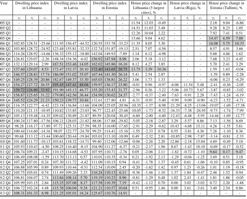
Stage 2. Analyzing the trends of real estate market in three Baltic States from the equilibrium perspective, it can be noted that in dwelling market during 2006 Q4 – 2008 Q4 there have been observed the build-up of the financial imbalances when dwelling prices were over the long-term equilibrium level (Fig. 7). In Estonian dwelling market the build-up phase has been identified in 2006 Q4, the peak – in 2007 Q2, and the ending phase – in 2007 Q3–2008 Q3. Whereas, in Latvian dwelling market the build-up of the financial imbalances was observed one quarter later than in Estonian market, the peak – in 2008 Q1, and the ending phase – in 2008 Q2–2008 Q4. The build-up of financial imbalances in Lithuanian dwelling market was identified only in 2007 Q2, the peak – in 2008 Q2, and the ending phase – in 2008 Q3–2008 Q4. Besides, it also should be noted that the largest growth of the dwelling price index was observed in Latvia suggesting about the largest financial imbalance in real estate market comparing to other Baltic countries. The house price changes in the Baltic countries capitals or 5 largest cities (Lithuania) demonstrate
no clear trends during the analyzed period (Table V).
-50 -40 -30 -20 -10 0 10 20 30 40 50 2 0 0 6 Q 1 2 0 0 6 Q 3 2 0 0 7 Q 1 2 0 0 7 Q 3 2 0 0 8 Q 1 2 0 0 8 Q 3 2 0 0 9 Q 1 2 0 0 9 Q 3 2 0 1 0 Q 1 2 0 1 0 Q 3 2 0 1 1 Q 1 2 0 1 1 Q 3 2 0 1 2 Q 1 2 0 1 2 Q 3 2 0 1 3 Q 1 Year D w e ll in g p r ic e i n d e x ( D P I) A
LTU DPI cyclical component LVA DPI cyclical component
EST DPI cyclical component DPI threshold
Fig. 7. The identification of dwelling market equilibrium level in the Baltic States.
Year Dwelling price index in Lithuania
Dwelling price index in Latvia
Dwelling price index in Estonia
House price change in Lithuania (5 largest
cities), %
House price change in Latvia (Riga), %
House price change in Estonia (Tallinn), %
yt τt ct yt τt ct yt τt ct yt τt ct yt τt ct yt τt ct
2005 Q1 - - - 11.54 12.03 -0.49 - - - 2.18 9.04 -6.86
2005 Q2 - - - 14.51 11.03 3.48 - - - 9.28 8.23 1.05
2005 Q3 - - - 12.26 10.04 2.22 - - - 7.92 7.41 0.51
2005 Q4 - - - 13.66 9.04 4.62 - - - 14.47 6.59 7.88
2006 Q1 102.85 128.51 -25.66 111.95 156.47 -44.52 120.55 153.78 -33.23 11.35 8.05 3.30 - - - 16.08 5.75 10.33
2006 Q2 103.80 128.72 -24.92 123.48 155.81 -32.33 132.74 151.87 -19.13 2.51 7.07 -4.56 - - - 8.57 4.91 3.66
2006 Q3 114.26 128.92 -14.66 136.32 155.12 -18.80 142.04 149.93 -7.89 1.14 6.12 -4.98 - - - 5.68 4.06 1.62
2006 Q4 126.81 129.07 -2.26 148.34 154.36 -6.02 156.92 147.94 8.98 2.06 5.18 -3.12 - - - 7.68 3.23 4.45
2007 Q1 132.13 129.14 2.99 167.51 153.46 14.05 162.02 145.86 16.16 8.12 4.27 3.85 - - - 5.70 2.41 3.29
2007 Q2 137.60 129.07 8.53 172.47 152.37 20.10 172.40 143.65 28.75 13.75 3.39 10.36 - - - 1.59 1.63 -0.04
2007 Q3 146.57 128.83 17.74 186.09 151.02 35.07 167.44 141.30 26.14 5.41 2.54 2.87 - - - -1.39 0.89 -2.28
2007 Q4 149.25 128.39 20.86 182.67 149.37 33.30 165.03 138.81 26.22 3.06 1.73 1.33 - - - -6.06 0.23 -6.29
2008 Q1 154.27 127.72 26.55 195.45 147.41 48.04 159.97 136.17 23.80 -0.01 0.96 -0.97 -6.06 -11.54 5.48 -2.41 -0.36 -2.05
2008 Q2 159.72 126.80 32.92 191.90 145.13 46.77 155.20 133.43 21.77 -2.96 0.26 -3.22 -5.06 -10.73 5.67 -3.87 -0.85 -3.02
2008 Q3 156.87 125.65 31.22 179.00 142.56 36.44 154.99 130.62 24.37 -2.77 -0.37 -2.40 -7.63 -9.91 2.28 -7.43 -1.24 -6.19
2008 Q4 145.52 124.29 21.23 150.23 139.77 10.46 132.61 127.80 4.81 -6.31 -0.91 -5.40 -9.99 -9.09 -0.90 -6.23 -1.52 -4.71
2009 Q1 116.35 122.77 -6.42 123.18 136.84 -13.66 104.09 125.05 -20.96 -10.35 -1.37 -8.98 -21.29 -8.25 -13.04 -19.07 -1.69 -17.38
2009 Q2 110.20 121.15 -10.95 110.82 133.85 -23.03 96.77 122.45 -25.68 -10.05 -1.73 -8.32 -34.33 -7.38 -26.95 -9.73 -1.74 -7.99
2009 Q3 105.13 119.48 -14.35 109.02 130.89 -21.87 89.59 120.04 -30.45 -6.60 -2.00 -4.60 -12.43 -6.48 -5.95 -14.46 -1.69 -12.77
2009 Q4 100.24 117.80 -17.56 106.21 128.03 -21.82 88.06 117.88 -29.82 -5.05 -2.18 -2.87 3.29 -5.57 8.86 7.13 -1.56 8.69
2010 Q1 98.28 116.17 -17.89 97.72 125.31 -27.59 98.35 116.00 -17.65 -2.91 -2.29 -0.62 10.43 -4.68 15.11 4.26 -1.35 5.61
2010 Q2 100.44 114.60 -14.16 98.07 122.77 -24.70 99.25 114.41 -15.16 -1.55 -2.33 0.78 0.55 -3.81 4.36 7.26 -1.10 8.36
2010 Q3 99.68 113.12 -13.44 100.60 120.44 -19.84 103.01 113.10 -10.09 0.49 -2.32 2.81 -10.85 -2.98 -7.87 -3.14 -0.81 -2.33
2010 Q4 101.60 111.73 -10.13 103.61 118.32 -14.71 99.40 112.06 -12.66 -0.06 -2.26 2.20 12.86 -2.18 15.04 4.69 -0.49 5.18
2011 Q1 105.93 110.43 -4.50 108.25 116.40 -8.15 104.90 111.27 -6.37 -0.21 -2.17 1.96 8.67 -1.43 10.10 -0.69 -0.17 -0.52
2011 Q2 106.74 109.21 -2.47 110.15 114.68 -4.53 107.95 110.71 -2.76 0.05 -2.06 2.11 -1.82 -0.72 -1.10 9.64 0.17 9.47
2011 Q3 106.49 108.08 -1.59 113.70 113.13 0.57 110.01 110.35 -0.34 0.21 -1.92 2.13 -1.29 -0.04 -1.25 3.69 0.51 3.18
2011 Q4 107.25 107.01 0.24 107.30 111.72 -4.42 111.09 110.15 0.94 -0.41 -1.78 1.37 -0.45 0.61 -1.06 -0.10 0.85 -0.95
2012 Q1 106.88 105.99 0.89 109.93 110.44 -0.51 112.54 110.09 2.45 -0.20 -1.62 1.42 0.97 1.23 -0.26 1.01 1.19 -0.18
2012 Q2 105.75 105.01 0.74 111.49 109.26 2.23 116.24 110.13 6.11 -0.36 -1.46 1.10 1.37 1.84 -0.47 2.46 1.52 0.94
2012 Q3 106.81 104.07 2.74 113.84 108.14 5.70 119.19 110.23 8.96 -0.81 -1.29 0.48 1.02 2.43 -1.41 1.81 1.86 -0.05
2012 Q4 105.99 103.15 2.84 115.25 107.08 8.17 117.58 110.39 7.19 -0.42 -1.12 0.70 0.00 3.02 -3.02 0.72 2.20 -1.48
2013 Q1 106.72 102.24 4.48 115.38 106.04 9.34 121.21 110.57 10.64 0.51 -0.95 1.46 0.00 3.61 -3.61 3.40 2.54 0.86
2013 Q2 108.31 101.33 6.98 121.25 105.01 16.24 125.67 110.76 14.91 - - - -
Notes: denotes the build-up and the ending phases of dwelling market boom, while – the peak of dwelling market boom. Calculating dwelling price index in all three Baltic countries the base is 2010 = 100. House price change is calculated as a change over a quarter.
The recent trends in the dwelling market in all three Baltic States signal about the increasing dwelling prices and possible next build-up of the financial imbalances in real estate market.
So, summarizing it can be stated that the build-up of financial imbalances in loan and real estate markets in three Baltic countries occurred at the same time and the loan boom caused the financial imbalances in the real estate market.
Stage 3. The research results show that the financial imbalances in the Baltic countries loan markets were simultaneous during 2006-2010, except the Lithuania where the loan market boom ended one year earlier than in Latvia and Estonia. Analyzing the trends of real estate market in three Baltic States, it can be noted that in dwelling market during 2006 Q4–2008 Q4 there have been observed the build-up of the financial imbalances. The results of this study are similar to the results that were obtained by [20] and [22]. The economy downturn in 2009-2010 in all three Baltic countries worsened banks borrowers’ abilities to meet theirs obligations to banks, which lead to a sharp growth of non-performing loans and consequently caused commercial banks losses and increased special provisions. In addition, large banks losses and reduced economic activity lead to banks capital problems and reduced aggregate credit growth.
Besides, falling real estate prices during economy recession in 2009-2010 reduced the value of companies and collateral, whereas, a lower value of collateral means that companies and households will receive less credits. In addition, more restrictive lending policy of commercial banks created difficulties for weaker companies to obtain credits. During economy recession high leveraged companies reduced their demand for banks credits and lead to slowdown of aggregate credit growth. Falling credit supply forced companies and households to reduce both investment and consumption, which resulted in a decrease of output in the short-run and had adverse effect on economy of Baltic States in the long-run.
Stage 4. Analyzing the build-up of financial imbalances in loan and real estate markets in the Baltic countries from 2005-2007 perspective, it can be stated that the potential build-up of loan and real estate market boom could be predicted in 2002-2003 and the specific macro-prudential tools could be introduced in time in order to prevent the build-up of financial imbalances. [2] distinguish the main macro-prudential policy instruments, which may be devoted to prevention of the build-up of financial imbalances: tightening capital requirements, limiting credit expansion, introducing both liquidity and leverage ratios, controlling the
degree of maturity transformation. [7] discuss the major policy options (monetary, fiscal, and macro-prudential tools) to deal with financial imbalances. They distinguish the main macroeconomic policy tools: monetary measures (tightening of monetary policy, e.g., through a rise in key policy rates) and fiscal measures (tightening of fiscal policy (removal of incentives for borrowing, e.g., mortgage interest tax deductibility, subsidies/guarantees for mortgages, corporate tax shield provided by debt) and financial sector taxation)). [7] also distinguish a wide range of regulatory policy tools: macro-prudential measures (reserve requirements, differentiated capital requirements, higher risk weights, liquidity requirements, dynamic provisioning, limits on credit growth, limits on loan-to-value ratio, limits on debt-to-income ratio, credit concentration limits, net open position limits, maturity mismatch regulations) and monitoring measures (intensified surveillance on vulnerable, stress testing and stronger disclosure requirements).
VI. CONCLUSIONS
Summarizing the identification of the build-up of financial imbalances in the Baltic States results, the following conclusions can be formulated:
1.The financial imbalances in the Baltic countries loan markets have been build-up simultaneous during the period of 2006-2010, except the Lithuania where the loan market boom ended one year earlier than in Latvia and Estonia. The main causes of loan markets boom in three Baltic countries are the following: less restrictive lending policy of commercial banks, very low level of the financial deepening, the transition processes in these countries, etc.
2.Analyzing the equilibrium level in real estate market in three Baltic States, it can be noted that in dwelling market during 2006 Q4–2008 Q4 there have been observed the build-up of the financial imbalances when dwelling prices were over the long-term equilibrium level. The loan market boom in all three Baltic countries caused the financial imbalances in the real estate market.
3.The research results show that the potential build-up of loan and real estate market boom in all three Baltic countries could be predicted in 2002-2003 and the specific policy options (monetary, fiscal, and macro-prudential tools) could be introduced in time in order to prevent the build-up of financial imbalances.
REFERENCES
[1] I. Bunda and M. C. Zorzi, “Signals from housing and lending booms,”
Emerging Markets Review, vol. 11, no. 1, pp. 1-20, March 2010.
[2] V. Borgy, L. Clerc, and J.-P. Renne, “Asset-price boom-bust cycles and
credit: What is the scope of macro-prudential regulation?” Working papers 263, Banque de France, 2009.
[3] A. Barajas, G. Dell’Ariccia, and A. Levchenko, “Credit booms: the
good, the bad, and the ugly,” Unpublished manuscript, International Monetary Fund (Washington, DC), 2009.
[4] A. Tornell and F. Westermann, “Boom-bust cycles in middle income
countries: Facts and explanation,” IMF staff papers, Palgrave Macmillan, vol. 49, pp. 111-155, 2002.
[5] D. Serwa, “Identifying multiple regimes in the model of credit to
households,” National Bank of Poland, Working paper no. 99, pp. 1-28, 2011.
[6] E. G. Mendoza and M. E. Terrones, “An anatomy of credit booms:
Evidence from macro aggregates and micro data,” IMF working papers 08/226, International Monetary Fund, 2008.
[7] G. D. Ariccia, D. Igan, L. Laeven, H. Tong, B. Bakker, and J.
Vandenbussche, “Policies for macrofinancial stability: How to deal with credit booms,” IMF staff discussion notes 12/06, International Monetary Fund, pp. 1-46, 2012.
[8] International Monetary Fund, “Are credit booms in emerging markets a
concern?” World Economic Outlook, Chapter 4, 2004.
[9] M. B. Brzezina, “Lending booms in Europe’s periphery: South-western
lessons for Central-Eastern members,” Macroeconomics 0502002,
Econ WPA, 2005.
[10] M. Schularick and A. M. Taylor, “Credit booms gone bust: Monetary
policy, leverage cycles, and financial crises, 1870-2008,” American
Economic Review, vol. 102, no. 2, pp. 1029-1061, 2012.
[11] P. O. Gourinchas, R. Valdes, and O. Landerretche, “Lending booms:
Latin America and the world,” Economia, spring issue, pp. 47-99,
2001.
[12] S. Elekdag and Y. Wu, “Rapid credit growth: Boon or boom-bust?”
IMF working papers 11/241, International Monetary Fund, pp. 1-42, 2011.
[13] A. Geršl and J. Seidler, “Excessive credit growth as an indicator of
financial in stability and its use in macroprudential policy,” Czech National Bank, financial stability report 2010/2011, pp. 112-122.
[14] B. Égert, P. Backé, and T. Zumer, “Credit growth in Central and
Eastern Europe – New (over) shooting stars?” European central bank working paper no. 687, 2006.
[15] C. Cottarelli, G. D. Ariccia, and I. V. Hollar, “Early birds, late risers,
and sleeping beauties: Bank credit growth to the private sector in
Central and Eastern Europe and the Balkans,” Journal of Banking and
Finance, vol. 29, no. 1, pp. 83-104, 2005.
[16] C. Duenwald, N. Gueorguiev, and A. Schaechter, “Too much of a good
thing? Credit booms in transition economies: The cases of Bulgaria, Romania, and Ukraine,” IMF working paper 05/128, 2005.
[17] F. Boissay, O. C. Gonzalez, and T. Kozluk, “Is lending in Central and
Eastern Europe developing too fast?” in Financial Development,
Integration and Stability, edited by K. Liebscher, Edward Elgar eds.,
2006.
[18] G. Kiss, M. Nagy, and B. Vonnák, “Credit growth in Central and
Eastern Europe: Convergence or boom?” MNB working papers 2006/10, Magyar Nemzeti Bank the Central Bank of Hungary, 2006.
[19] J. Vandenbussche, U. Vogel, and E. Detragiache, “Macroprudential
policies and housing prices – A new database and empirical evidence for Central, Eastern, and Southeastern Europe,” IMF working papers WP/12/303, International Monetary Fund, pp. 1-36, 2012.
[20] O. Ertuganova, “Baltic States: Credit crunch or return to equilibrium
level?” in International Conference on Applied Economics – ICOAE,
pp. 161-165, 2010.
[21] P. Honohan, “Banking system failures in developing and transition
countries: Diagnostics and prediction,” BIS working paper no. 39, January 1997.
[22] V. Deltuvaitė, “Paskolų rinkos pusiausvyros lygio vertinimas: Lietuvos
atvejis,” Ekonomika ir Vadyba: Aktualijos ir Perspektyvos, to be
published.
[23] R. J. Hodrick and E. C. Prescott, “Postwar U.S. business cycles: An
empirical investigation,” Journal of Money, Credit, and Banking, vol.
29, no. 1, February 1997, pp. 1-16, 1997.
[24] P. Hilbers, I. O. Robe, C. Pazarbasioglu, and G. Johnsen, “Assessing
and managing rapid credit growth and the role of supervisory and prudential policies,” IMF working paper WP/05/151, 2005.
Vilma Deltuvaitė is a lecturer at Department of Finance, Faculty of Economics and Management, Kaunas University of Technology, Lithuania. The
a is Laisves av. 55, LT-44309 Kaunas,
Lithuania. She has Accounting and Logistics specialist, Chief financial officer, Head of Logistics department, General manager (CEO) working experience in private enterprises. She obtained a doctoral degree in Social Sciences (Management) at
Kaunas University of Technology in 2013. Her r are
systemic risk management in the banking sector, banking crises, banking sector financial stability, cross-border contagion risk.
ddress