ISSN (Online): 2320-9364, ISSN (Print): 2320-9356
www.ijres.org Volume 4 Issue 9
ǁ
September. 2016
ǁ
PP. 01-05
Study and Application of TSP Based on Genetic Algorithm
Zongjie Du
1, Shulin Sui
11
(Department college Of Mathematics & Physics/Qingdao University of Science & Technology University Name, China)
Abstract:
Traveling salesman problem ( TSP ) has been proved a non-deterministic polynomial complete problems. Theoretically the enumeration can not only solve the problem, but can find out the optimal solution of the problem. It is almost impossible that using common enumeration to find the optimal solution in such a large search space. Therefore all kinds of optimization algorithm has been arisen to solve the traveling salesman problem. In this paper we study the traveling salesman problem based on genetic algorithm, we will transform the shortest path problem between cities to the offspring which can been got through crossover and mutation from parent, genetic algorithm circulate this process until the end. Through the numerical experiment on 31 cities, we can get the shortest path and the corresponding traversal sequence between the 31 cities. This crossover strategy based on genetic algorithm can retain the same pattern of parent, and we also generate better individual than the parent by larger probability.
Keywords:
Traveling salesman problem ( TSP ), genetic algorithm , shortest pathI.
INTRODUCTION
Traveling salesman problem is a typical combinatorial optimization problem, the problem show the simplified form and the focus of many complex problems in the field of generalization [1]. Effective solution this problem is classified as a scientific problem in twenty-first Century. Solution this problem has important theoretical significance and practical application value. Traveling salesman problem has wide application in many fields such as network communication, scheduling and chain stores of goods delivery paths. Therefore the rapid and effective solution the traveling salesman problem has important practical value.
As we all known any kind of algorithm is not perfect. Each algorithm is constantly improved and optimized, and each has its own scope of application. In the same way genetic algorithm has its advantages and disadvantages [2]. In this paper, we study traveling salesman problem based on genetic algorithm, the genetic algorithm which start from point set as the starting point has good global search capability. In this way we can quickly search the solution space of all solutions by the inherent parallelism, this distributed computing can approach to the optimal solution quickly [3].
II.
INTRODUCTION
THE
TRAVELING
SALESMAN
PROBLEM
AND
GENETIC
ALGORITHM
A. Introduction the Traveling Salesman Problem and Genetic Algorithm
Traveling salesman problem is an optimization problem. Assuming we know the mutual distance between cities, now a traveling salesman must traverse the cities, and each city can only be visited once, finally traveling salesman must return to the starting city[4]. How to arrange the path order can get the shortest length of the travel? That is to say how to seek a shortest Hamiltonian circuit.
In terms of [5] graph theory to restatement of the problem. there is a graph g( , )v e ,
v
represent vertex set which is named the city,e
represent the line between the cities,ij
d
regard as the distance between cityi
v
and cityj
v
, then traveling salesman problem is for Ncities1 2 ( , , , n)
v v v L v to seek access sequence
1 2 ( , , , )n
t t t L t , and we record tn1t1 as the Hamiltonian circuit. The mathematical model of
minId t i t t, 1 , i1, 2,n is the traveling salesman problem.
Therefore we need to find the shortest path from all around the travel path, the number of paths is (n1)! from the initial point, so the traveling salesman problem is a permutation problem, Through enumeration
of
n1 !
travel paths to find the shortest path of the travel paths.B. Basic principles of genetic algorithm
The genetic algorithm which is a parallel random search optimization method was put forward in 1962 by Professor Holland of Michigan University in the United States. Genetic algorithm evolves constantly to get a new generation of population by going through with the rules of selection, reproduction, crossover and mutation operations, and making the search process approach to the optimal solution based on the fitness function. After several generations of evolution, the algorithm converges to the optimal solution or satisfactorysolution. The genetic algorithm mainly includes the coding design, setting the initial group, designing the fitness function, setting control parameters and designing genetic operations (including population size, hereditary frequency, crossover probability and mutation probability, etc.). The basic operation of genetic algorithm is divided into three steps [6].
(1) select operation
The selection operation choose new population from the old population by a certain probability of fitness. The better fitness, the greater probability of being selected. The purpose of selection operation is that the optimized individual can inheritance to the next generation. Genetic algorithm can set the number of population in the initial and randomly choose parent, then genetic algorithm choose the better parent after a round of operation.
(2) crossover operation
The crossover operation exchange genetic information of chromosome, the offspring will be generated by swapping and rearranging genetic information from two parents. The crossover operation procedure is as follows, firstly the crossover point randomly select in the parent generation, then check whether there is a conflict. Lastly cross operation change conflict nodes until no conflict between the generations.
A:1100: 0101 1111 crossover A: 1100:0101 0000 B:1111: 0101 0000 B: 1111:0101 1111 (3) mutation operation
Mutation operation randomly choose one of the individuals from the population. In order to produce a better individual, mutation operation randomly select a point in the chromosome to mutation.
A: 1100 0101 1111 mutation A: 1100 0101 110
Basic operation process of genetic algorithm: (1) initialization
Set the initial iteration number t0, and the maximum number of iterations T, randomly generated M individual as the initial population P
0 .(2) individual evaluation
The problem is encoded into chromosome, and definite the fitness function, computing the individual fitness of P t
population.(3) selection operation
The selection operator acts on the population. The purpose of selection operation is that the optimized individual can inheritance to the next generation.
(4) crossover operation
The crossover operator acts on the population. The called crossover is the operation of generating new individuals by swapping and rearranging genetic information from two parents.
(5) mutation operation
The mutation operator is acts on the population. We can get the next generation P t
1
by
P t carrying out selection, crossover and mutation.
(6) termination judgment
If tT, then the evolutionary process of the individual.
III.
APPLICATION
OF
GENETIC
ALGORITHM
IN
TRAVELING
SALESMAN
PROBLEM
A. Problem description
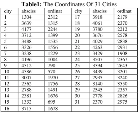
Table1: The Coordinates Of 31 Cities city absciss ordinat city absciss ordinat 1 1304 2312 17 3918 2179 2 3639 1315 18 4061 2370 3 4177 2244 19 3780 2212 4 3712 1399 20 3676 2578 5 3488 1535 21 4029 2838 6 3326 1556 22 4263 2931 7 3238 1229 23 3429 1908 8 4196 1004 24 3507 2367 9 4312 790 25 3394 2643 10 4386 570 26 3439 3201 11 3007 1970 27 2935 3240 12 2562 1756 28 3140 3550 13 2788 1491 29 2545 2357 14 2381 1676 30 2778 2826 15 1332 695 31 2370 2975 16 3715 1678
B. Application and realization of genetic algorithm in traveling salesman problem
Firstly the genetic algorithm carry out initial operation and set the fitness function. In order to facilitate description of the path, we use 1 to 31 represent the 31 cities.
Secondly we randomly select two paths as the parent, two offspring can be formed through crossover and mutation.
Then according to the predefined fitness function which represent the shortest path, we take the fitness function to rank. In the first round of the calculation, the numerical experiment selected 100 population which can generate 100 offspring. We use the fitness function to sort the 200 paths, and select the best 100 offspring as the next parents. The iterative continue to operation until the optimal path is got.
Finally we change the number of iterations and check whether the obtained path converges to the optimal path.
The minimum distance is set as the fitness function [8], the expression is as follow: ( ,1) min
( ,1) (1 )
max min 0.0001
m
len i len
fitness i
len len
Set judgment function as follow:
( ,1) *
fitness i jc jcrand alpha
Select the relatively optimal individual and retain the individual which its path is shortest. Then genetic algorithm enter the next iteration.
C. The results analysis
1000 1500 2000 2500 3000 3500 4000 4500
500 1000 1500 2000 2500 3000 3500 4000
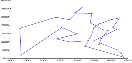
From Figure 1 we can see that the spatial coordinates of the 31 provincial cities are not regular, that is to say we can not use a numerical optimization method to find the optimal path.
We can find that there will be lots of lines between the 31 cities, the number of the calculation is 30!. We can not find the optimal solution through a simple numerical optimization.
We can discuss the greedy method, branch and bound method, list optimization method and the simulated annealing method to solve these problems. We consider genetic algorithm which has the ability to more efficient of global optimization [9].
Firstly we consider the 1000th time of iteration, and we find that the relative optimal paths of the 1000 times are as the figure 2.
1000 1500 2000 2500 3000 3500 4000 4500 500
1000 1500 2000 2500 3000 3500 4000
Fig. 2. 1000 iteration relative optimal path between the 31 cities
The 1000 relative optimal path length is 1.811245 10 4.
Relative optimal path as follow: 12 14 13 6 5 3 18 22 21 20 24 23 7 10 9 8 4 2 16 17 19 25 26 27 28 30 31 1 15 29 11
0 100 200 300 400 500 600 700 800 900 1000
1.8 2 2.2 2.4 2.6 2.8 3 3.2 3.4x 10
4
Fig. 3. 1000 iteration path length variation between the 31 cities
Through the constant iteration, figure 3 show the better offspring gradually into convergence by the superior of the fittest. When the number of iteration set 1000 times, the path length gradual tend to 1.8 10 4 .
According to the theory of genetic algorithm, the more the number of iterations, the more excellent offspring can get [10]. We can see that when iterated 2000 times, the relative optimal path condition is as the figure4.
1000 1500 2000 2500 3000 3500 4000 4500 500
1000 1500 2000 2500 3000 3500 4000
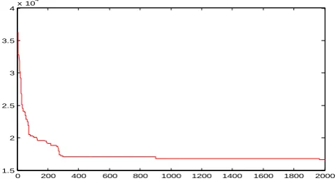
The change of superior path length is as the figure5.
0 200 400 600 800 1000 1200 1400 1600 1800 2000 1.5
2 2.5 3 3.5
4x 10
4
Fig. 5. 2000 iteration path length variation between the 31 cities
We can see from the figure above, the path length change is a convergent process. The 2000 relative optimal path length is 1.662658 10 4.
The relative optimal path of iteration 2000th times is: 5 16 3 22 21 26 28 27 31 30 25 24 20 18 17 19 23 11 29 1 15 14 12 13 6 7 2 9 10 8 4
IV.
CONCLUSION
The effectiveness of genetic algorithm to solve combinatorial optimization problems has been acknowledged for scientific researchers. In order to improve the solution performance and expand the application field, scientific researchers constantly take effort to research and explore [11]. In this paper through analyzing the principle and advantages of genetic algorithm, we study traveling salesman problem based on genetic algorithm. Through numerical experiment the genetic algorithm can find the optimal solution or suboptimal solution, this shows that the algorithm has better optimization performance.
Although genetic algorithm can find a better solution in a relatively short time, genetic algorithm prone to premature convergence phenomenon. The process of finding the optimal solution needs to be iterated many times, so we can adjust some parameters to improve the speed and precision of searching for the optimal solution.
REFERENCES
[1]. Haonan Ren, Using genetic algorithm to solve TSP problem[D]. Shandong: Shandong University, 2008. [2]. Yang Peng, Principle and application of genetic algorithm[M]. Beijing: National Defence Industry Press, 1999.
[3]. Jingwei Gao, Xu Zhang, Realization of genetic algorithm for solving traveling salesman problem[J]. The computer age, (2), 2004, 19-21.
[4]. Janghua Chen, Aiwen Lin, Ming Yang, Jian Gong, Research progress of genetic algorithm for solving TSP problem[J]. Journal of Kunming University of Science and Technology(Science and Technology), 28(4), 2003, 9-13.
[5]. Hehua Liu, Chao Cui, Jing Chen, An improved genetic algorithm to solve traveling salesman problem[J]. Journal of Beijing institute of technology, 33(4), 2013, 390-393.
[6]. Minghai Yao, Na Wang, Lianpeng Zhao, Improved simulated annealing and genetic algorithm for solving TSP problems[J]. Computer Engineering and Applications, 49(14), 2013, 60-65.
[7]. GuiPing Dai, yong Wang, Yarong Hou, Traveling salesman problem solved based on genetic algorithm and its system [J]. Microcomputer information, 26(1), 2010, 15-19.
[8]. Dengying Xuan, Fulin Wang, Minhui Gao, Haizhi Ma. A improve fitness function of genetic algorithm to [J]. Mathematics in practice and theory, 45(16), 2015, 232-238.
[9]. Yumei Lei, Solution scheme of large scale TSP problem based on Improved Genetic Algorithm[J]. Computers and modernization, (2), 2005, 34-38.
[10]. Sicai Zhang, Fangxiao Zhang, An improved method of fitness function of genetic algorithm[J]. Computer applications and software, 23(2), 2006, 108-110.