https://doi.org/10.5194/amt-11-6511-2018 © Author(s) 2018. This work is distributed under the Creative Commons Attribution 4.0 License.
Boundary-layer water vapor profiling using differential
absorption radar
Richard J. Roy, Matthew Lebsock, Luis Millán, Robert Dengler, Raquel Rodriguez Monje, Jose V. Siles, and Ken B. Cooper
Jet Propulsion Laboratory, California Institute of Technology, Pasadena, California, USA Correspondence:Richard J. Roy ([email protected])
Received: 3 July 2018 – Discussion started: 15 August 2018
Revised: 14 November 2018 – Accepted: 22 November 2018 – Published: 6 December 2018
Abstract. Remote sensing of water vapor in the presence of clouds and precipitation constitutes an important obser-vational gap in the global observing system. We present ground-based measurements using a new radar instrument operating near the 183 GHz H2O line for profiling water va-por inside of planetary-boundary-layer clouds, and develop an error model and inversion algorithm for the profile re-trieval. The measurement technique exploits the strong fre-quency dependence of the radar beam attenuation, or dif-ferential absorption, on the low-frequency flank of the wa-ter line in conjunction with the radar’s ranging capability to acquire range-resolved humidity information. By com-paring the measured differential absorption coefficient with a millimeter-wave propagation model, we retrieve humidity profiles with 200 m resolution and typical statistical uncer-tainty of 0.6 g m−3 out to around 2 km. This value for hu-midity uncertainty corresponds to measurements in the high-SNR (signal-to-noise ratio) limit, and is specific to the fre-quency band used. The measured spectral variation of the dif-ferential absorption coefficient shows good agreement with the model, supporting both the measurement method as-sumptions and the measurement error model. By performing the retrieval analysis on statistically independent data sets corresponding to the same observed scene, we demonstrate the reproducibility of the measurement. An important trade-off inherent to the measurement method between retrieved humidity precision and profile resolution is discussed.
Copyright statement. © 2018 California Institute of Technology. Government sponsorship acknowledged.
1 Introduction
is accompanied by decreased differential absorption, making the profiling capabilities of this radar coarser than the 183 to 193 GHz DAR. Furthermore, the surface returns in both cloudy and clear-sky areas make a DAR measurement of the total water column possible.
The DAR approach has two unique aspects that com-plement existing methods for remotely sensing water va-por. First, because of its ranging capabilities it has precise height registration, unlike passive sounding whereby weight-ing functions can encompass broad swaths of the atmo-sphere. Second, in contrast with other methods the DAR sig-nal increases with increasing cloud water content and pre-cipitation, with the obvious caveat that the radar signal-to-noise ratio (SNR) will decrease from attenuation as the beam penetrates into the volume. The DAR therefore nicely com-plements the infrared and microwave sounding techniques, as well as differential absorption and Raman lidar tech-niques that are commonly used to remotely sense water va-por from the ground (Whiteman et al., 1992; Wulfmeyer and Bösenberg, 1998; Spuler et al., 2015), with a notable airborne DIAL system being the Lidar Atmospheric Sens-ing Experiment (LASE) (Browell et al., 1998). Importantly, millimeter-wave transparency in clouds allows for airborne or spaceborne measurements of lower tropospheric humidity in cloudy scenes, while DIAL systems typically cannot mea-sure inside boundary-layer clouds due to high optical thick-ness.
In addition to primary applications in profiling water va-por within clouds, the instrument architecture discussed here represents an important application of recent advances in solid-state G-band technology to meteorological radar. In-deed, there has been lingering interest within the atmospheric remote sensing community for decades in utilizing G-band radar for cloud and precipitation studies, with earlier at-tempts hampered by limited sensitivity due to available tech-nology (Battaglia et al., 2014). The addition of G-band re-flectivity measurements to multi-frequency radar systems, for example a dual-frequency W- and Ka-band system, could provide significantly more information than additional mea-surements at a lower frequency because the scattering prop-erties at G band for typical cloud particle sizes are not of Rayleigh character.
Here we present ground-based measurements using a 167 to 174.8 GHz DAR, provide in-depth measurement error analysis with emphasis on the role of background noise power, and develop a retrieval algorithm based on perform-ing least squares fits of a spectroscopic model to the data. The retrieved profiles constitute the first active remote sens-ing measurements of water vapor profiles inside of clouds, and open up possibilities for a variety of scientific studies, in-cluding investigation of in-cloud humidity heterogeneity and the coupled relationship between boundary-layer clouds and thermodynamic profiles.
2 Measurement basis and method 2.1 Differential absorption radar
The DAR technique (Lawrence et al., 2011; Millán et al., 2014; Cooper et al., 2018) utilizes range-resolved radar echoes at multiple carrier frequencies in the vicinity of a gaseous absorption line to probe the frequency-dependent optical depth between two points along the radar line-of-sight. The radar echoes, or returns, may originate from cloud hydrometeors or, in the case of an airborne system, from the Earth’s surface as well, enabling total column optical depth measurements. For closely spaced transmission frequencies near the absorption line center, the hydrometeor scattering properties vary little, while the gaseous absorption exhibits strong frequency dependence. By comparing with a known propagation model, these measurements can be employed to retrieve range-resolved density profiles of the absorbing molecule. Furthermore, because of the differential nature of the measurement, one does not require absolute calibration of the radar receiver in order to obtain absolute density val-ues for the absorbing molecule. In the case of a calibrated receiver, both range-resolved density profiles of the absorb-ing molecule and microphysical properties of the reflectabsorb-ing medium can be retrieved.
Assuming negligible multiple scattering, the radar echo power received from a collection of scatterers filling the beam at a distanceris
Pe(r, f )=C(f )Z(r, f )r−2e−2τ (r,f ), (1) whereC(f )includes the frequency dependence of the radar hardware (e.g., transmit power and gain), Z(r, f ) is the (unattenuated) reflectivity, andτ (r, f ) is the one-way opti-cal depth including contributions from gaseous and particu-late extinction. Taking the ratio of powers for two different rangesr1andr2=r1+Rand assuming frequency indepen-dence of the reflectivity and particulate extinction, we find Pe(r2, f )
Pe(r1, f )
=Z(r2) Z(r1)
r
1 r2
2
e−2β(r1,r2,f )R, (2) where
β(r1, r2, f )=
τ (r2, f )−τ (r1, f ) R
= 1 R
r2
Z
r1
" X
j
ρj(r)κj(r, f )+βpart(r)
#
dr (3)
is the average absorption coefficient betweenr1andr2,ρj(r)
is the density of the gas component with label j,κj(r, f )
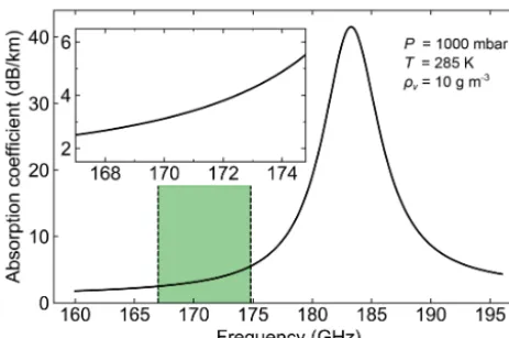
Figure 1.Gaseous absorption coefficient (one-way) calculated us-ing the model from Read et al. (2004) and the parameters listed in the figure. The green shaded region and inset highlight the 167 to 174.8 GHz transmission band for this work.
Restricting our analysis to millimeter-wave propagation near the 183 GHz water vapor absorption line, the sum over gaseous absorption terms can be replaced byρv(r)κv(r, f )+ βgas,bg(r), where the subscript v corresponds to water vapor andβgas,bgis the background gas absorption coefficient due to all other components, which is assumed to be frequency-independent. Assuming that pressure and temperature vary slowly compared to the length scale R, we can therefore write Eq. (3) as
β(r1, r2, f )=ρv(r1, r2)κv(f )+βgas,bg(r1, r2)
+βpart(r1, r2), (4)
where the overbar symbol implies taking the mean value be-tweenr1andr2. Thus, we see that measuring the frequency-dependent contribution to the optical depth between r1 and r2 reveals the average water vapor density given the known absorption line shapeκv(f ). Figure 1 shows the fre-quency dependence of the gaseous absorption coefficient ρvκv(f )+βgas,bgin the vicinity of the 183 GHz water vapor line forP =1000 mbar,T =285 K, andρv=10 g m−3. For this work, we utilize the millimeter-wave propagation model from the EOS Microwave Limb Sounder (Read et al., 2004). The 167 to 174.8 GHz transmission band is highlighted in green, as well as shown in the inset of Fig. 1, revealing a dif-ferential absorption coefficient of 3 dB km−1for 10 g m−3of water vapor.
Important to the validity of this DAR method is the domi-nance of gaseous differential absorption over particulate dif-ferential absorption, since we assume thatβpartis frequency-independent. To investigate this for boundary-layer clouds, we perform Mie scattering calculations for liquid spheres and integrate the scattering parameters over DSDs corresponding to clouds and rain for a range of mean diameters. For the DSD, we use a modified gamma distribution of the form
N (D)= N0 0(ν)
D
Dn
ν−1 1 Dn
e−D/Dn, (5)
where N0 is a normalization factor with units of particle number per volume that fixes the total liquid water content L, ν is the shape parameter, which is set to 4 for clouds and 1 for rain, and Dn is the characteristic diameter. For
rain we enforce an additional constraint thatN0=x1D1
−x2
n ,
wherex1=26.2 mx2−4andx2=1.57 have been determined in previous studies by comparing to observations (Abel and Boutle, 2012). This allows the entire rain distribution to be determined by the liquid water content. The rain rate is cal-culated from this distribution by using the terminal velocity relation from Beard (1976).
The results are shown in Fig. 2, where we plot the differen-tial particulate extinction,1βpart(f )=βpart(f )−βpart(f0), as a function ofDn. Heref0=167 GHz corresponds to the low-frequency end of the transmission band. In Fig. 2a, the corresponding rain rate is displayed on the upper horizontal axis. For the cloud species, the normalization parameterN0is not fixed by any additional constraint, and is therefore deter-mined at eachDnto fixL, which is set here to 500 mg m−3.
To find the differential particulate extinction for other values ofL, one can linearly scale the values in Fig. 2b. Clearly for precipitation scenarios, the differential extinction from rain is more than 2 orders of magnitude smaller than that from wa-ter vapor. For clouds in the limit of small diamewa-ter, the differ-ential particulate extinction asymptotes to the Rayleigh value of1βpartRayleigh=6πLIm(Kw)(f−f0)/(ρwc)=0.2 dB km−1 forf =174.8 GHz, whereρwis the density of liquid water, Kw=(m2w−1)/(m2w+2),mw is the complex refractive in-dex of water, andcis the speed of light. For larger values of Dn, the differential extinction is enhanced by a resonant
fea-ture characteristic of Mie scattering. Thus, for thick clouds withLas large as 500 mg m−3, especially those that contain drizzle drops which tend to lie near this resonant size, there are important bias considerations that warrant future study in order to establish the application of DAR in these partic-ular scenarios. Specifically, to mitigate the potential biases stemming from scattering by hydrometeors, the unattenuated reflectivity can be used to distinguish clouds from precipita-tion, and the frequency-dependent scattering effects can be modeled and incorporated in the retrieval.
Figure 2.Differential particulate extinction coefficients for (a)rain and (b)cloud. In the case of rain, the DSD characteristic diameter
Dn determines the liquid water content and hence the rain rate, while for clouds we fixL=500 mg m−3. The legend in(a)gives the
corresponding frequencies in GHz.
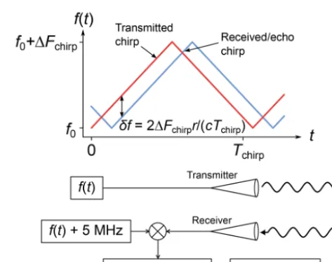
duration Tchirp. After scattering off of a target at a dis-tance r from the radar, the received chirp is delayed in time by an amount 2r/c, leading to a fixed frequency offset of δf =21Fchirpr/(cTchirp)relative to the transmitted fre-quency chirp. By downconverting the received signal using the transmitted frequencyf (t )shifted by 5 MHz for conve-nient amplification and detection, the fixed frequency offset between transmitted and received chirps is converted into a constant frequency signal in the intermediate frequency (IF) stage. Signal processing techniques are then used to convert the IF time-domain signal to a range-resolved power spec-trum. In the IF power spectrum, the zero-range point is lo-cated at 5 MHz and the echo power from a rangeRis located atfIF(r)=5 MHz±δf (r), where the positive(negative) sign applies for decreasing(increasing) frequency chirps.
Our system utilizes state-of-the-art millimeter-wave com-ponents designed at the Jet Propulsion Laboratory (JPL) and builds on years of FMCW radar development for security and planetary science applications (Cooper et al., 2011, 2017). The architecture is similar to that presented in an earlier work (Cooper et al., 2018) which demonstrated the DAR technique between 183 and 193 GHz, but modified to transmit in the 167 to 174.8 GHz band, in which transmission is not prohib-ited by international regulations (NTIA, 2015), to perform narrow-bandwidth frequency chirps, and to provide a 5 MHz offset of the zero-range radar signal from zero frequency within the IF band. The IF offset is helpful for future cali-brated power measurements because of various effects that inhibit accurate power estimation near zero frequency. The radar has an average transmit power of 140 mW, is outfit-ted with a 6 cm primary aperture with corresponding gain of 40 dB, and uses a frequency chirp of bandwidth1Fchirp= 60 MHz and durationTchirp=1 ms, resulting in a range
res-Figure 3.Basic FMCW radar schematic. See Sect. 2.2 for discus-sion.
Table 1.Hardware and radar signal acquisition parameters used in this work. The noise figure reported is for a complex radar signal detected using a double-sideband front-end mixer.
Parameter Value Unit
Transmit frequency 167–174.8 GHz
Transmit power 140 mW
Noise figure <8 dB
Primary aperture diameter 6 cm
Antenna gain 39 dB
Far-field beam width (FWHM) 1.9 degrees
Side lobe level −23 dB
Chirp bandwidth 60 MHz
Chirp time 1 ms
Range resolution 2.5 m
To process the downconverted radar signal, we first ple it using an analog-to-digital converter (ADC) with a sam-pling frequency of 20 MHz for the 1 ms duration of the chirp. Then we apply a Hanning window in the time domain be-fore performing a fast Fourier transform (FFT) to obtain the range-resolved power spectrum. Application of the Hanning window reduces side lobes from bright targets as well as the large transmit–receive leakage signal that is always present at zero range. For the radar parameters listed above, the cor-responding conversion factor from IF frequency to the target range isδf (r)/r=400 kHz km−1.
2.3 Power measurement uncertainty
The starting point for assessing the achievable precision in humidity using DAR measurements is the statistical uncer-tainty of the radar power measurements themselves. Until this point, we have ignored the role of background noise power in the radar spectrum, which is an important factor in any realistic receiver. In general, the noise power within a given radar range bin Pn is proportional to the sum of the receiver noise temperature and the antenna temperature, which itself is proportional to the scene brightness tempera-ture. By considering the simultaneous coherent detection of noise (Pn) and radar echo (Pe) power, one can show that the statistical uncertainty of thedetectedpower,Pd=Pe+Pn, is given by (see Appendix A)
σd= 1
p Np
Pe2+2PePn+Pn2
1/2
, (6)
whereNpis the number of radar pulses transmitted.
In order to accurately determine the frequency-dependent optical depth between two range bins, it is critical to obtain a separate measurement of the background noise power in the absence of radar echoes and subtract this off of Pd. To see why this is, consider Eq. (2) with the left-hand side replaced by Pd(r2, f )/Pd(r1, f ), which is equivalent to interpreting the detected power as the true echo power, setZ(r2)=Z(r1)
for simplicity, and consider the limitPePn (i.e.,Pd→ Pn). In this case we would find that exp(−2β(r1, r2, f )R)→ 1 regardless of the actual value of Pe, and thus would in-correctly estimate a vanishing water vapor density, when in fact it is the echo power which has vanished. Similarly, for modest values of the SNR≡Pe/Pn, this would lead to a sys-tematic underestimate of the true humidity. Therefore, af-ter subtracting the separate noise power measurement from Pd we obtain a measurement of Pe with total uncertainty σe=(σd2+σn2)1/2, whereσn=Pn/pNpis the noise power measurement uncertainty (see Eq. 6 withPe=0). The rela-tive uncertainty in the measured echo power is therefore
σe Pe = 1 p Np
1+ 2 SNR+
2 SNR2
1/2
. (7)
As will be discussed in Sect. 3, the range dimension is pur-posefully oversampled in our measurements, allowing us to decrease the statistical power uncertainty at a given range by averagingNbadjacent range bins. The resulting relative power uncertainty is given by
σe Pe
= ξ(Nb) p
NpNb
1+ 2 SNR+
2 SNR2
1/2
, (8)
whereξ(Nb)≥1 is a factor of order unity accounting for covariances between adjacent range bins that arise due to applying a window function to the time-domain radar sig-nal before transforming to Fourier space. For the Hanning window used in this work, this function is given byξ(Nb)=
1+Nb−1
Nb 8 9
1/2
.
2.4 Inversion algorithm for profile retrieval
Under the simplifying assumptions introduced in Sect. 2.1, and assuming that pressure and temperature are known as a function of range, the inverse problem to retrieve hu-midity can be solved directly. The implications of the lat-ter assumption are explored in Appendix C. To invert the radar spectra, we consider a set of measured echo powers Pe(ri, fj) for ranges {r1, r2, . . ., rm} and transmission
fre-quencies{f1, f2, . . ., fNf}, whereri+1−ri =1ris the radar
range resolution. We note that in most circumstances we em-ploy a retrieval step sizeR that is larger than 1r, since, as we will show below, the precision in our retrieved humidity scales favorably with total optical depth and hence with in-creasingR. Then, given a step size such thatR=ri+S−rifor
some integerS, we form the frequency-dependent measured quantity
γi(fj)= −
1 2Rln
" r
i+S
ri
2P
e(ri+S, fj)
Pe(ri, fj)
#
(9)
for each starting rangeri. From Eq. (2), we see that we can
perform-ing a least squares fit of the function ˆ
γ (f )=ρκv(f )+B (10)
to the measurements for each i, where B is a frequency-independent offset containing information about dry air gaseous absorption, particulate extinction, and the relative reflectivity of the two ranges in question. We drop the v subscript on the water vapor density in the above equa-tion for simplicity of notaequa-tion. The resulting humidity es-timates {ρ1, ρ2, . . ., ρm−S}have a corresponding range axis
{r1, r2, . . ., rm−S}, whereri =(ri+ri+S)/2, and have
asso-ciated uncertainties determined from the fitting procedure. Using standard error propagation, the estimated uncer-tainty in the measured quantityγi(fj)defined in Eq. (9) is
σγi(fj)=
1 2R σe Pe
ri+S,fj
!2 + σe
Pe
ri,fj
!2
1/2
. (11)
In order to derive a simple analytical expression for the rel-ative uncertainty in the retrieved humidity, we restrict our-selves for the moment to considering two transmission fre-quencies,f1andf2. In this case, we can combine Eqs. (2), (4), and (9) to obtain the humidity directly,
ρ(ri)=
κv(f2)−κv(f1)
−1
γi(f2)−γi(f1)
, (12)
with the associated relative uncertainty σρ ρ r i = 1 21τ X
j=1,2
σe Pe r
i+S,fj
!2
+ σe Pe
r
i,fj
!2
1/2
, (13)
where1τ =
κv(f2)−κv(f1)ρ(ri)Ris the differential
op-tical depth for f1 andf2 between range bins ri and ri+S.
Equation (13) reveals that there are three linked quantities determining the sensitivity of the system: (1) the magnitude of the DAR signal quantified by1τ, (2) the statistical uncer-tainty of the power measurements given by the quadrature sum of relative errors in Eq. (13), and (3) the relative uncer-tainty in the derived value for the humidity. Thus, given a set of measured echo powers and a specific value for the hu-midity, there is a trade-off between spatial resolution of the retrieval and relative uncertainty in the humidity estimate.
An important and subtle point regarding the uncertainty in the measured quantityγi(fj)is that Eq. (11) relies on a
Tay-lor expansion in the relative errorσe/Pe, and therefore is only valid for measurements with SNR above some critical value that depends on the number of measurementsNp. Because there is no closed-form expression for the probability distri-bution function (PDF) ofγi(fj), we resort to a Monte Carlo
analysis, which is described in Appendix B, to generate the
relevant PDFs for the parameters used in this work numeri-cally. From this analysis, we find that forNp=2000 pulses andNb=11 averaged bins, the Taylor expansion method is accurate for measurements with SNR>−10 dB.
We note here that it is typical of differential absorption systems to utilize only two frequencies: one online and one offline. However, in this work we are concerned with vali-dating both the spectroscopic model used and the radar hard-ware itself, which could be subject to unknown frequency-dependent systematic effects. The regression approach dis-cussed above thus provides for a robust comparison of the measured frequency dependenceγi(fj)with the model
ˆ
γ (f ), while a two-frequency approach would mask incon-sistencies between measurements and model, or systematic hardware effects, since the two free parametersρ andB are fully determined given two frequency points. Furthermore, a distributed set of frequencies allows for the possibility of ex-tending retrievals deeper in range for moist atmospheres, as frequencies closer to the line center will be attenuated more strongly, and can be excluded from the fits described above when the critical SNR value is reached.
3 Boundary-layer measurements and analysis 3.1 Radar characteristics, spectra, and filtering
In this section we report on measurements performed at JPL on 15 March 2018 using the proof-of-concept differ-ential absorption radar described in Sect. 2.2. For these measurements, we implement a new signal processing tech-nique for real-time noise floor characterization, utilizing a triangle-wave frequency chirp (i.e., bidirectional) instead of a sawtooth-wave chirp (i.e., unidirectional). According to FMCW radar principles, the echo spectrum switches from residing on the low- to the high-frequency side of the zero-range signal (i.e., 5 MHz) for increasing and decreasing lin-ear frequency chirps, respectively. As shown in Fig. 4a, this fast switching of the chirp direction alternately exposes the noise floor on each side of the zero-range point within the IF band, and provides accurate and nearly continuous esti-mation of the system noise power and the passive signal cor-responding to the scene brightness temperature at each fre-quency bin. This technique is especially advantageous for airborne/spaceborne applications, as the brightness tempera-ture of the observed scene can change on fast timescales due to different surface types (e.g., ocean versus land) and from the presence or absence of clouds.
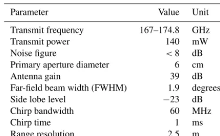
Figure 4.DAR measurement spectra.(a)The bidirectional frequency chirp technique provides for accurate, real-time characterization of the background noise floor within the radar’s IF band, with no loss of measurement duty cycle. Here the detected power spectrum for
fj=167 GHz is shown. The IF frequency to range conversion factor is 400 kHz km−1.(b)Echo power spectra normalized to their value
at 100 m for the 12 transmission frequencies. The large variability in the signals near 1.4 km indicates the system reaching the noise floor. (c)Echo power spectra after averagingNb=11 adjacent bins, and filtered for points with SNR>−10 dB.(d)Measurement relative error
(blue circles) for all traces in(c)compared with the statistical model (Eq. 8, dashed black line).
experimental sequence is as follows: first, we perform 40 frequency chirps at a given transmission frequency before switching to another frequency, which takes 1 ms. The re-ceived signal is downconverted to baseband, digitized in an ADC, and processed in real time as described in Sect. 2.2. We achieve a system duty cycle of>90 %, resulting in a to-tal measurement/observation time of≈25 s.
By subtracting the respective noise floors from the increas-ing and decreasincreas-ing frequency chirp measurements (Fig. 4a), and subsequently combining the mirrored spectra, we obtain our estimate of the echo power spectra. In Fig. 4b, we plot the echo power spectra scaled byr2for the 12 transmission frequencies before bin averaging, which reveals the range de-pendence of the quantity Z(r)exp(−2τ (r, f )). Each spec-trum is normalized to its value at 100 m. Thus, we observe the differential absorption due to water vapor directly from the spreading of the spectra with increasing range, whereby for a particular range, the plotted values increase monoton-ically with decreasing transmit frequency. After averaging
the quantityri2Pe(ri, fj)within a swath of sizeNb=11, we filter the spectra based on the Monte Carlo analysis in Ap-pendix B, keeping only those points with SNR>−10 dB, and are left with the smoothed profiles shown in Fig. 4c. Fig-ure 4d shows the relative error in the binned (Nb=11) echo power measurement (blue circles) plotted against the mea-sured SNR for all 12 frequencies. The meamea-sured values agree very well with those predicted by Eq. (8) (black dashed line), indicating that our statistical model based on speckle noise, which underlies the Monte Carlo simulations implemented in this work, is accurate.
3.2 Water vapor profile retrieval
Figure 5.Water vapor profile retrieval for DAR spectra from Fig. 4.(a)Three examples of least-squares fits of the millimeter-wave propaga-tion model to DAR measurements. Artificial offsets are imposed in order to plot all three on the same graph.(b)The retrieved profile exhibits roughly constant absolute humidity error until SNR≈10 dB (1 km). See Sects. 2.4 and 3.2 for retrieval details. The green line shows the saturated water vapor density range dependence using a near-surface temperature of 11◦C and lapse rate of 6◦C km−1. The shaded regions correspond to deviations of±2◦C.
we form the 12 quantitiesγi(fj)for each startingri in the
set{r1, r2, . . ., rm−S}, and perform a least-squares fit of the
functionγ (f )ˆ to the data at each range point. Note that the retrieved water vapor density ρi is related only to the
dif-ference between the value of the fitted function at 174.8 and 167 GHz, while the offset is related to particulate extinction and hydrometeor reflectivity, and is disregarded in this work. The pressure and temperature dependence of the absorption line shape is included in the fitting model using reported val-ues at the surface from a nearby weather station, and as-suming an exponential pressure profile with a scale height of 7.5 km and a temperature lapse rate of 6◦C km−1. We note that for the relatively short vertical extents of the pro-files from these ground measurements (e.g., 1.4 sin 30◦km for Figs. 4 and 5), the retrievedρvalues are quite insensitive to the assumed thermodynamic profiles (see Appendix C).
An important element of the DAR technique in general is utilizing an accurate model for the absorption line shape. Ex-amples of line shape fits to the data are shown in Fig. 5a for three different values of SNR, with arbitrary offsets imposed on the three traces to permit simultaneous plotting. To as-sign SNR values to these points, we compute the mean SNR for the 12 frequencies atri andri+S, and use the smaller of
the two. Clearly the millimeter-wave model accurately cap-tures the frequency dependence of the measurements, which is supported quantitatively by the typical reduced chi-square values of χred2 ≈1 for these fits. The retrieved water vapor density profile is shown in Fig. 5b, where the range ri
as-signed to each fitted valueρi is the midpoint ofri andri+S.
Also plotted here is an estimate of the saturation vapor den-sity given our lapse rate assumption. This profile is consis-tent with a cloud base between 400 and 600 m and shows qualitatively good agreement with the expectation that the
relative humidity is approximately 100 % in liquid cloud lay-ers. Note that because the retrieved values correspond to the mean humidity betweenri andri+S, we effectively retrieve
the profile convolved with a box of sizeR (200 m here). For this retrieval, the absolute humidity errors lie between 0.55 and 0.60 g m−3 until around 1 km (SNR≈10 dB), where the error steadily increases until the final retrieval point at 1.25 km withσρ=2.9 g m−3. The value ofσρ in the
high-SNR regime (i.e., the first 1 km) remains roughly constant, even thoughρvaries by a factor of 3, since the absolute hu-midity error is independent of the huhu-midity itself, and de-pends only on the differential mass extinction cross section κv(174.8 GHz)−κv(167 GHz), the retrieval step sizeR, and the power measurement uncertainty (see Eq. 13).
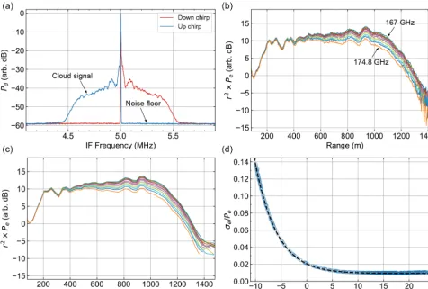
Figure 6.Retrievals for different cloud and precipitation conditions.(a)Averaged DAR power spectra (Nb=11) for light rain near the
surface, with a cloud extending from 1 to 2 km.(b)Retrieved humidity profiles for two independent data sets corresponding to the same scene from (a). (c)Averaged DAR power spectra (Nb=11) for heavy precipitation near the surface with strong particulate extinction. (d)Independent retrievals from two data sets for the scene in(c).
Given a measured range-resolved echo power spectrum, what retrieval range resolution can we achieve for a spec-ified minimum retrieval precision? As discussed briefly in Sect. 2.4, the relative error in the retrieved humidity σρ/ρ
(see Eq. 13) for a given power measurement uncertainty varies inversely with the differential optical depth, and thus depends on both the retrieval step sizeR (i.e., retrieval res-olution) used andthe absolute value of the humidityρ. Al-ternatively, one can look at the absolute error and rearrange Eq. (13) to find that, for a given pair of frequencies and power measurements at two ranges, the product ofσρandRis
con-stant. Hence, reducing the retrieval step size by some factor increases the absolute humidity error by the same factor. In future work we will implement a retrieval algorithm that has adaptive range resolution based on both the inherent signal (i.e., humidity) and the measurement noise.
4 Conclusions
A proof-of-concept humidity-profiling DAR operating be-tween 167 and 174.8 GHz has been constructed and tested
from the ground. The instrument builds on progress made in an earlier version operating between 183 and 193 GHz (Cooper et al., 2018), and employs a new signal process-ing technique for performprocess-ing real-time noise power spectrum characterization and subtraction, providing for higher accu-racy measurements of the radar echo power. A new direct inversion algorithm for retrieving humidity based on least squares fits to a spectroscopic model is applied to the mea-sured echo power spectra, showing close agreement between the measurement and model frequency dependence. The hu-midity profiles retrieved from two statistically independent measurement sets of the exact same scene are in close agree-ment, highlighting the reproducibility of the method. The un-certainties in the power measurements, which in part deter-mine the retrieved humidity uncertainty, agree very well with a statistical model based on radar speckle noise that incorpo-rates the effects of background noise subtraction and down-sampling, or binning, of the measured spectra.
transmit power. Important future steps for this instrument include validation of the measurement accuracy using co-incident measurements of humidity, pressure, and temper-ature (e.g., from radiosondes), and eventually testing from an airborne platform. Specifically, the surface returns while measuring from an airborne platform will be investigated for the retrieval of total column water within the bound-ary layer. A more significant augmentation of the system could include the addition of passive radiometric channels near the 183 GHz line. This would allow for continuous
mea-surement of vertical humidity profiles when transitioning be-tween clear-sky and cloudy areas, and opens the possibility to study biases in the humidity retrieved from radiometric mea-surements that are caused by scattering and emission from clouds.
Appendix A: Error in detected power
In this appendix, we derive the expression for the detected power uncertainty within a single radar range bin in the pres-ence of background noise (Eq. 6). To do so, we begin by as-suming that all targets within the scattering volume are ran-domly distributed, leading to the well-known Rayleigh fad-ing model for the received echo signal (Ulaby et al., 1982). In the context of FMCW radar, we then consider the re-ceived complex electric field amplitudeEi corresponding to
the ith frequency bin in the FFT spectrum, where we only consider the polarization direction that couples into the radar receiver. Within the Rayleigh fading model, it is shown that for Ei=E0,ieiφi, the modulus of the field amplitude E0,i
is normally distributed with zero mean and standard devia-tion σE, and the phase φi is uniformly distributed over the
interval[0,2π]. Alternatively, we can write the correspond-ing voltage in the receiver asVe,i=ai+ibi, whereaiandbi
are uncorrelated and are both normally distributed with zero mean. Then, from the expression converting electric field to power,Pe,i= |Ve,i|2=α|Ei|2, we find the probability
distri-bution function for the received echo power p(Pe,i≥0)=
1 hPe,ii
e−Pe,i/hPe,ii, (A1)
where the mean equals the variance and is given byhPe,ii =
2ασE2, α is a field-to-voltage conversion factor for the radar, andp(Pe,i<0)=0. Furthermore, we find thathai2i =
hbi2i = hPe,ii/2. Though not proven here, the Rayleigh
fad-ing model also shows that the expectation value of the re-ceived power fromNrandomly distributed targets is the sum of the expectation values of the individual target echo pow-ers.
Similarly, one can show that Gaussian white noise in the radar signal, which comes from both the scene brightness temperature and the radar electronics, results in a noise volt-age within the ith frequency bin of the FFT spectrum with Fourier coefficientVn,i=ci+idi, wherehcii = hdii =0 and
hc2ii = hdi2i = hPn,ii/2. We proceed towards deriving Eq. (6)
by considering the coherent detection of both the radar echo and noise signals. In this case, the detected voltage signal in the Fourier domain within the ith range bin is Vd,i=
Ve,i+Vn,i, and the detected power is Pd,i= |Vd,i|2. Using
the expectation values listed above, it is easy to show that
hPd,ii = hPe,ii + hPn,ii (A2)
and
Var(Pd,i)= hPe,ii + hPn,ii
2
. (A3)
Therefore, we recover Eq. (6) by computing the standard er-ror forNindependent measurements,σd2,i=Var(Pd,i)/N.
Appendix B: Monte Carlo Analysis
As discussed in Sect. 2.3, subtracting off the noise power contribution to the detected powerPdis critical for accurate humidity estimation. However, for low values of SNR, we clearly expect the result hPei = hPdi − hPni to be negative some of the time due to finite sampling, where “h· · ·i” de-notes the sample average. This is nonphysical. Therefore, in order to account for these finite sampling effects and the po-tential breakdown of standard error propagation whenσe/Pe is not small, we employ a Monte Carlo simulation of the DAR measurement. The PDF for the echo power received from randomly distributed hydrometeor targets within a sin-gle range bin is given by Eq. (A1). In order to generate random samples of the radar spectrum for transmission fre-quencyfj, we begin with an idealized spectrumhPe(ri, fj)i
for which we setC(f )=Z(r, f )=1 andρv(r)=constant, and sample the distribution (Eq. A1) at each range bin ri.
We then perform a fast Fourier transform (FFT) to obtain the corresponding time-domain radar signal, add the effects of background noise using Gaussian white noise, and apply a Hanning window. Taking the inverse FFT thus supplies a single random realization of a measuredPdspectrum. For the simulated spectra used in this work, we generateNp=2000 radar pulses with range resolution1r=2.5 m and average them to realize a single radar measurement. These values for Npand1rare the same parameters utilized in the field mea-surements presented in Sect. 3. We generate 10 000 averaged spectra for both Pd andPn, giving 10 000 random realiza-tions of the echo power measurement. For these simularealiza-tions, we usefj =167 GHz andρv=7.4 g m−3.
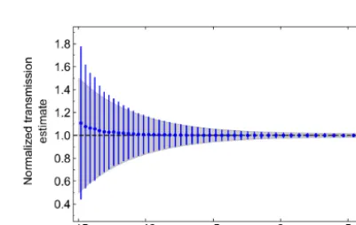
Our aim is to utilize the Monte Carlo simulations to inform where the Taylor expansion method for error propagation breaks down in our estimation ofσγi(fj), and thus provide
a criterion for filtering our measurements. To do so, we fix Nb=11 and the step sizeS=10 (i.e., 275 m) and compute the mean and standard deviation of the Monte Carlo proba-bility distribution for the two-way transmission between ri
and ri+S for each ri. Figure B1 shows the results, where
we plot the Monte Carlo mean value divided by the a priori two-way transmission used to generate the Monte Carlo re-sults, as a function of the SNR atri+S. The gray shaded area
represents the SNR-dependent errors predicted from Eq. (8). There are two notable deviations that arise for SNR values below 0.1: (1) the error estimated using the standard error propagation formalism begins underestimating the true stan-dard deviation calculated using the Monte Carlo ensemble, and (2) the mean of the Monte Carlo-generated distribution systematically overestimates the true two-way transmission. We note here that this point of departure between the naive error propagation estimate and that from the Monte Carlo distributions does not depend onNborS, but is determined by the number of independent pulses Np used to realize a single radar measurement. From these simulations, we con-clude that the standard error propagation model is sufficient for SNR>−10 dB. Therefore, after downsampling the mea-sured spectra withNb=11, we eliminate all measured val-ues with SNR<−10 dB, as described in Sect. 3.1.
Appendix C: Retrieval dependence on assumed pressure and temperature values
To assess the dependence of the retrieved humidity on tem-perature and pressure, we will consider again the case of the two-frequency measurement, using transmission frequencies f1=167 GHz andf2=174.8 GHz. Then, for a given start-ing rangeriand step sizeR, we use the measured quantities
γi(f1)andγi(f2)to solve for the mean humidity between the two ranges,
ρi=
γi(f2)−γi(f1) κv(f2, P , T )−κv(f1, P , T )
=γi(f2)−γi(f1) 1κv(P , T )
, (C1)
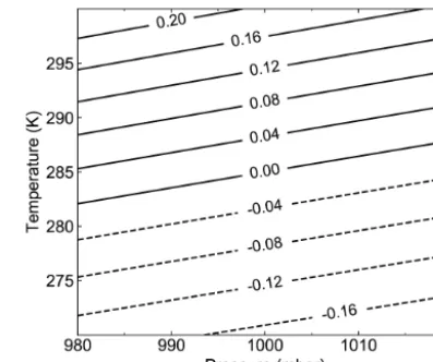
Figure C1.Humidity error for assumed temperature T0=285 K
and pressureP0=1000 mbar versus actual valuesT andP.
where we now explicitly writeκvas a function of temperature T and pressureP, and we have defined the differential mass extinction cross section1κv(P , T )for these two frequencies. Given reference values ofP0=1000 mbar andT0=285 K, and corresponding retrieved humidityρi,0, we calculate the error in our humidity estimate for different conditionsP and T as
ρi−ρi,0 ρi,0
=1κv(P0, T0) 1κv(P , T )
−1. (C2)
Competing interests. The authors declare that they have no conflict of interest.
Acknowledgements. This research was supported by NASA’s Earth Science Technology Office under the Instrument Incubator Pro-gram, and was carried out at the Jet Propulsion Laboratory (JPL), California Institute of Technology, Pasadena, CA, USA, under contract with the National Aeronautics and Space Administration. Richard J. Roy’s research was supported by an appointment to the NASA Postdoctoral Program at JPL, administered by Universities Space Research Association under contract with NASA.
Edited by: Murray Hamilton
Reviewed by: Gerald Mace and two anonymous referees
References
Abel, S. J. and Boutle, I. A.: An improved representation of the rain-drop size distribution for single-moment microphysics schemes, Q. J. Roy. Meteor. Soc., 138, 2151–2162, 2012.
Battaglia, A., Westbrook, C. D., Kneifel, S., Kollias, P., Humpage, N., Löhnert, U., Tyynelä, J., and Petty, G. W.: G band atmo-spheric radars: new frontiers in cloud physics, Atmos. Meas. Tech., 7, 1527–1546, https://doi.org/10.5194/amt-7-1527-2014, 2014.
Beard, K. V.: Terminal Velocity and Shape of Cloud and Precipita-tion Drops Aloft, J. Atmos. Sci., 33, 851–864, 1976.
Browell, E., Ismail, S., and Grant, W.: Differential absorption lidar (DIAL) measurements from air and space, Appl. Phys. B, 67, 399–410, 1998.
Browell, E. V., Wilkerson, T. D., and Mcilrath, T. J.: Water vapor differential absorption lidar development and evaluation, Appl. Optics, 18, 3474–3483, 1979.
Cooper, K. B., Dengler, R. J., Llombart, N., Thomas, B., Chattopad-hyay, G., and Siegel, P. H.: THz Imaging Radar for Standoff Per-sonnel Screening, IEEE T. Thz. Sci. Techn., 1, 169–182, 2011. Cooper, K. B., Durden, S. L., Cochrane, C. J., Monje, R. R.,
Den-gler, R. J., and Baldi, C.: Using FMCW Doppler Radar to Detect Targets up to the Maximum Unambiguous Range, IEEE Geosci. Remote S., 14, 339–343, 2017.
Cooper, K. B., Monje, R. R., Millán, L., Lebsock, M., Tanelli, S., Siles, J. V., Lee, C., and Brown, A.: Atmospheric Humidity Sounding Using Differential Absorption Radar Near 183 GHz, IEEE Geosci. Remote S., 15, 163–167, 2018.
Lawrence, R., Lin, B., Harrah, S., Hu, Y., Hunt, P., and Lipp, C.: Ini-tial flight test results of differenIni-tial absorption barometric radar for remote sensing of sea surface air pressure, J. Quant. Spec-trosc. Ra., 112, 247–253, 2011.
Lebsock, M. D., Suzuki, K., Millán, L. F., and Kalmus, P. M.: The feasibility of water vapor sounding of the cloudy boundary layer using a differential absorption radar technique, Atmos. Meas. Tech., 8, 3631–3645, https://doi.org/10.5194/amt-8-3631-2015, 2015.
Millán, L., Lebsock, M., Livesey, N., Tanelli, S., and Stephens, G.: Differential absorption radar techniques: surface pressure, At-mos. Meas. Tech., 7, 3959–3970, https://doi.org/10.5194/amt-7-3959-2014, 2014.
Millán, L., Lebsock, M., Livesey, N., and Tanelli, S.: Differen-tial absorption radar techniques: water vapor retrievals, Atmos. Meas. Tech., 9, 2633–2646, https://doi.org/10.5194/amt-9-2633-2016, 2016.
NTIA: Manual of Regulations and Procedures for Federal Radio Frequency Management, National Telecommunications & Infor-mation Administration (NTIA), Revision of the May 2013 Edn., 2015.
Read, W. G., Shippony, Z., and Snyder, W.: EOS MLS forward model algorithm theoretical basis document, Jet Propulsion Lab-oratory, JPL D-18130/CL#04-2238, Pasadena, CA, USA, 2004. Spuler, S. M., Repasky, K. S., Morley, B., Moen, D., Hayman, M.,
and Nehrir, A. R.: Field-deployable diode-laser-based differen-tial absorption lidar (DIAL) for profiling water vapor, Atmos. Meas. Tech., 8, 1073–1087, https://doi.org/10.5194/amt-8-1073-2015, 2015.
Ulaby, F., Moore, R., and Fung, A.: Microwave Remote Sensing: Active and Passive, Vol. II, Addison-Wesley Publishing Com-pany, Inc., Reading, Massachusetts, 1982.
Whiteman, D. N., Melfi, S. H., and Ferrare, R. A.: Raman lidar system for the measurement of water vapor and aerosols in the Earth’s atmosphere, Appl. Optics, 31, 3068–3082, 1992. Wulfmeyer, V. and Bösenberg, J.: Ground-based differential