Profit Analysis of a Computer System With
Priority to Software Replacement over
Hardware Repair Subject to Maximum
Operation and Repair Times
Ashish Kumar and S.C. Malik
Department of Statistics, M.D. University, Rohtak-124001, Haryana (India) Email: [email protected]
Abstract
The goal of this paper is to determine some reliability and economic measures of a computer system in which h/w and s/w components fails independently direct from normal mode. The reliability model of two identical-units is developed considering computer system as a single- unit. Initially one unit is operative and the other unit is kept as cold standby. A single server is provided immediately to the system for conducting PM, repair and replacement of the components. The unit undergoes for PM after MOT directly from normal mode. The repair of the unit is done only at h/w failure subject to maximum repair time ( MRT). If repair of the unit is not possible up to a MRT, the component is replaced by new one giving some replacement time. However, only replacement of the component in the unit is made at software failure. The priority to software replacement is given over h/w repair. The failure times of the h/w and s/w components are distributed exponentially while the distribution of preventive maintenance, repair and replacement are taken as arbitrary. By adopting semi-Markov process and regenerative point technique , some important result for a particular case are also obtained to study the graphical behaviour of MTSF, availability and profit of the system model.
Key Words: Computer System, Independent H/W and S/W Failure, Priority, Maximum Operation and Repair Time, Preventive Maintenance and Profit Analysis.
2000 Mathematics Subject Classification: 90B25 and 60K10 Introduction:
hardware platforms. Recently, Malik and Anand (2010) proposed a reliability model of a computer system with independent hardware and software failures. In this model, hardware components are replaced by new one at their failure with some replacement time. However, only replacement of software components is made. Also, not much work related to the reliability modeling and profit analysis of computer systems with integrated hardware and software components has been visualized so far in the literature.
While considering the above facts and to fill up the gap, the present paper is designed to evaluate some reliability and economic measures of a computer system in which h/w and s/w components fails independently direct from normal mode. The reliability model of two identical-units is developed considering computer system as a single- unit. Initially one unit is operative and the other unit is kept as cold standby. A single server is provided immediately to the system for conducting PM, repair and replacement of the components. The unit undergoes for PM after MOT directly from normal mode. The repair of the unit is done only at h/w failure subject to maximum repair time (MRT). If repair of the unit is not possible up to a MRT, the component is replaced by new one giving some replacement time. However, only replacement of the component in the unit is made at software failure. The priority to software replacement is given over h/w repair. The failure times of the h/w and s/w components are distributed exponentially while the distribution of preventive maintenance, repair and replacement are taken as arbitrary.
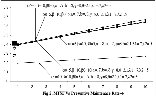
The random variables are independent and uncorrelated to each other. The switch devices and repair are perfect. To carry out profit analysis, various reliability characteristics such as mean sojourn times, mean time to system failure (MTSF), availability, busy period of the server due to hardware and software failures, expected number of replacements due to hardware and software failure, expected number of visits by the server and finally the profit considering various costs are determined by adopting semi-Markov process and regenerative point technique. Some important results for a particular case are also obtained to study the graphical behaviour of MTSF, availability and profit of the system model.
Notations
E : The set of regenerative states
NO : The unit is operative and in normal mode Cs : The unit is in cold standby
a/b : Probability that the system has hardware / software failure λ1/λ2 : Constant hardware / software failure rate
α0
: Maximum constant rate of Operation Time
β0 : Maximum constant rate of Repair Time.
Pm/PM : The unit is under preventive Maintenance/ under preventive maintenance continuously from previous state
WPm/WPM : The unit is waiting for preventive maintenance/ waiting for preventive maintenance continuously from previous state HFur/HFUR : The unit is failed due to hardware and is under repair / under repair continuously from previous state
HFwr / HFWR : The unit is failed due to hardware and is waiting for repair/ waiting for repair continuously from previous state
SFurp/SFURP : The unit is failed due to the software and is under replacement/ under replacement continuously from previous state
SFwrp/SFWRP : The unit is failed due to the software and is waiting for
replacement / waiting for replacement continuously from previous state h(t) / H(t) : pdf / cdf of replacement time of unit due to software
g(t) / G(t) : pdf / cdf of repair time of the hardware m(t)/ M(t) : pdf / cdf of replacement time of the hardware f(t) / F(t) : pdf / cdf of the time for PM of the unit
qij (t)/ Qij(t) : pdf / cdf of passage time from regenerative state i to a regenerative state j or to a failed state j without visiting any other regenerative state in (0, t] pdf / cdf : Probability density function/ Cumulative density function
qij.kr (t)/Qij.kr(t) : pdf/cdf of direct transition time from regenerative state i to a regenerative state j or to a failed state j visiting state k, r once in (0, t] μi(t) : Probability that the system up initially in state Si∈ E is up
at time t without visiting to any regenerative state
Wi(t) : Probability that the server is busy in the state Si upto time ‘t’without making any transition to any other regenerative state or returning to the same state via one or more non-regenerative states.
mij : Contribution to mean sojourn time (μi) in state Si when system transit directly to state
Sj so that i ij j
m
μ
=
and mij =*
'
( )
(0)
ij ijtdQ t
= −
q
/© : Symbol for Laplace-Stieltjes convolution/Laplace convolution
~ / * : Symbol for Laplace Steiltjes Transform (LST) / Laplace Transform (LT) ' (desh) : Used to represent alternative result
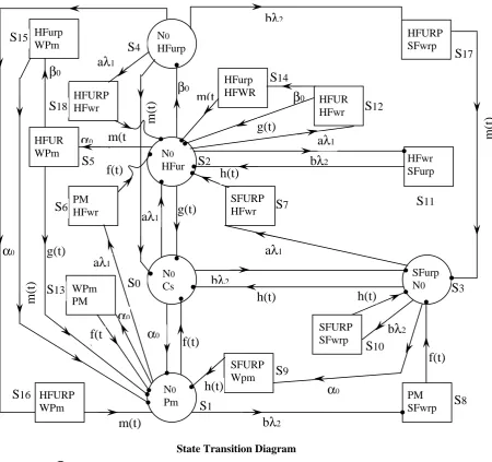
Considering these symbols, the following are possible transition states of the system model: S0 = (No, Cs), S1 = (No, Pm), S2 = (No, HFur), S3 = (No,SFurp), S4 = (No,HFurp), S5 = (HFUR,Wpm), S6 = (HFwr, PM), S7 = (SFURP, HFwr), S8 = (PM, SFwrp), S9 = (SFURP, WPm), S10 = (SFURP, SFwrp), S11 = (HFwr,SFurp)
S12 = (HFUR, HFwr) S13 = (WPm, PM), S14 = (HFWR,HFurp), S15 = (HFurp,WPM), S16= (HFURP,WPm), S17 = (HFURP, SFwrp) S18 = (HFURP, HFwr)
Transition Probabilities and Mean Sojourn Times
Simple probabilistic considerations yield the following expressions for the non-zero elements
∞=
∞
=
0
(
)
)
(
q
t
dt
Q
p01=
α
λ
λ
1α
2 00
+ +
b
a
, p02=λ
λ
α
λ
0 2 1 1 + +b
a
a
,p03 =
α
λ
λ
1λ
2 02
+ +
b
a
b
p10 = f*( aλ1+bλ2+α0) , p16 =
α
λ
λ
1λ
2 01
+ +
b
a
a
[ 1- f*( aλ1+bλ2+α0)] = p12.6
p18=
α
λ
λ
1λ
2 02
+ +
b
a
b
[ 1- f*( aλ1+bλ2+α0)]= p13.8
p1.13=
α
λ
λ
1α
2 00
+ +
b
a
[ 1- f *( aλ1+bλ2+α0)] = p11.13, p20 = g*( aλ1+bλ2+α0+β0),
p24 =
β
α
λ
λ
1β
2 0 00 + + +
b
a
[ 1- g*
( aλ1+bλ2+α0+β0)] ,
p25 =
β
α
λ
λ
1α
2 0 0 0+ + +
b
a
[ 1- g*
( aλ1+bλ2+α0+β0)]
p2.11 =
β
α
λ
λ
1 2λ
0 02
+ + +
b
a
b
[ 1- g*( aλ1+bλ2+α0+β0)]
p2.12 =
β
α
λ
λ
1λ
2 0 01 + + +
b
a
a
[ 1- g*( aλ1+bλ2+α0+β0)]
p30 = h*( aλ1+bλ2+α0), p37 =
α
λ
λ
1λ
2 01
+ +
b
a
a
[ 1- h*( aλ1+bλ2+α0)]= p32.7
p39 =
α
λ
λ
1α
2 00
+ +
b
a
[ 1- h *( aλ1+bλ2+α0)]= p31.9 p40 = m*( aλ1+bλ2+α0),
p3,10 =
α
λ
λ
1λ
2 02
+ +
b
a
b
[ 1- h*( aλ1+bλ2+α0)]= p33.10, p51 = g*(β0),
p5,15 = 1- g*(β0),p4.16 =
λ
λ
α
α
0 2 1 0 + +b
a
[ 1- m*( aλ1+bλ2+α0)]= p41.16, p62 = f*(0),p72 = h*(0),p83 = f *(0), p91 = h *(0), p10.3 = h*(0), p11,3 = h*(0),
p4,17 =
α
λ
λ
1λ
2 02
+ +
b
a
b
[ 1- m*( aλ1+bλ2+α0)] = p43.17, p12.2 = g*(β0), p12.15 = 1- g*(β0),
p13.1 = f*(0), p4.18 =
α
λ
λ
1λ
2 01
+ +
b
a
a
[ 1- m*( aλ1+bλ2+α0)]= p42.18,
p14.2 = m*(0), p15.1 = m*(0), p16.1 = m*(0), p17.3 = m*(0), p18.2 = m*(0),
p21.5 =
β
α
λ
λ
1α
2 0 00
+ + +
b
a
[ 1- g*
( aλ1+bλ2+α0+β0)] g*(β0)
p21.5,15 =
β
α
λ
λ
1α
2 0 00
+ + +
b
a
[ 1- g*
( aλ1+bλ2+α0+β0)][1- g*(β0)]
p22.12 =
β
α
λ
λ
1 2λ
0 01
+ + +
b
a
a
[ 1- g*p22.12,14 =
β
α
λ
λ
1 2λ
0 01
+ + +
b
a
a
[ 1- g*( aλ1+bλ2+α0+β0)][1- g*(β0)] (2)
It can be easily verified that p01+p02+p03 = p10+p16+p18+p1.13 = p20+p24+p25+ p2,11+p2.12 = p30+p37+p39+p3,10 = p40+p4.16+p4.17+ p4.18 = p5.1+ p5.15= p62= p72 = p83 = p91 = p10.3
= p11.2 =p12.2 + p12.14 = p13.1 = p14.2 =p15.1 = p16.1 = p17.3 =p18.2 = p10 +p12.6+ p11.13 +p13.8 = p20 +p24 +p21.5 +p2.11
+p21.5,15 +p22,12 +p22.12,14 = p30+p31.9+p32.7+p33.10 = p40 +p41.16+ p42.18+ p43.17= 1 (3)
The mean sojourn times (μi) is the state Si are
μ0 =
α
λ
λ
1
2
0
1
+
+
b
a
, μ1 =
α
α
λ
λ
1
+
2
+
0
+
1
b
a
, μ2 =
β
θ
α
λ
λ
1
2
0
01
+
+
+
+
b
a
,μ3 =
β
α
λ
λ
1
+
2
+
0
+
1
b
a
, μ4 =
γ
α
λ
λ
1
+
2
+
0
+
1
b
a
,
μ
1' =1
α
,' 3
μ
=1
β
,' 4
μ
=1
γ
,Z=
μ
2' =3
2
3
(
)
(
)
(
1
2
0
0
) (
0
)
1
0
1
2
0
0
2
2
2
(
)
{2 (
1
2
0
0
)
1
2
0
0
0
(
1
2
0
0
)
0
}
2
2
(
)
(
1
2
0
0
) (
0
)
2
2
1
2
0
0
2
(
0
) (
1
2
0
0
) (
1
0
)(
1
2
a
b
a
a
b
a
b
a
b
a
b
b
b
a
b
a
b
a
b
a
a
b
λ
λ α β
λ α θ
λ
λ α β
θ β
λ
λ α β
β
θ λ
λ α β
β
λ
λ α β
θ
θ
λ
λ α β
θ β
λ
λ
λ
λ α θ β
θ β
λ
λ α β
λ α
λ
λ α
+
+ +
+
+
+
+ +
+
+
+ +
+
+ +
+
+
+
+ +
+ −
−
+
+ +
+
−
+
+ + +
+
+
+ +
+
+
+
+
0
0
)
3
3
(
)
(
)
[(
1
2
0
0
)
0
(
1
2
0
0
)
1
2
0
0
3
(
1
2
0
0
) (
0
)]
2
2
3
(
)
(
1
2
0
0
) (
1
2
0
0
)
0
a
b
a
b
a
b
a
b
a
b
a
b
θ β
θ β
λ
λ α β
λ
λ α β
λ
λ α θ β θ
λ
λ α β
θ β
θ β
λ
λ α β
λ
λ θ α β
+ +
+
+
+ +
+
+ +
−
+
+ + +
+
+
+ +
+
+
+
+
+ +
+
+ + +
(4) Also 0 03 0201
+
m
+
m
=
μ
m
m
10+
m
16+
m
18+
m
1.13=
μ
12 12 . 2 11 . 2 25 24
20
+
m
+
m
+
m
+
m
=
μ
m
m
30+
m
37+
m
39+
m
3.10=
μ
34 19 . 4 18 . 4 17 . 4
40
+
m
+
m
+
m
=
μ
m
m
51+
m
5.16=
μ
5m
11.14+
m
11.3=
μ
1112 2 . 12 15 .
12
+
m
=
μ
m
m
62=
μ
6m
72=
μ
7,m
83=
μ
8,m
91=
μ
9,m
10.3=
μ
10, 1 13 . 11 8 . 13 6 . 1210
+
m
+
m
+
m
=
μ
′
m
(say) 2 14 , 11 . 23 11 . 23 15 , 12 . 22 12 . 22 16 , 5 . 21 5 . 21 2420+m +m +m +m +m +m +m =μ′
m (say) 3 10 . 33 7 . 32 9 . 31
30
+
m
+
m
+
m
=
μ
′
m
(say),m
40+
m
42.19+
m
43.18+
m
41.17=
μ
4′
(
say
)
(5) Reliability and Mean Time to System Failure (MTSF)φ
0(t) = Q01(t)Ⓢφ
1(t) + Q02(t)Ⓢφ
2(t)+ Q03(t)Ⓢφ
3(t)φ
1(t) = Q10(t)Ⓢφ
0(t) + Q16(t)+ Q1.13(t) + Q18(t)φ
2(t) = Q20(t)Ⓢφ
0(t) + Q24(t) Ⓢφ
4(t) +Q25(t)+ Q2.11(t)+ Q2.15(t)φ
3(t) = Q30 (t)Ⓢφ
0(t) + Q37(t) + Q39(t) + Q3,10φ
4(t) = Q4,0 (t)Ⓢφ
0(t) + Q4,17(t) + Q4.18(t) +Q4,19 (6)Taking LT of above relation (6) and solving for
φ
~
0(
s
)
We haveR*(s) =
s
s
)
(
~
1
−
φ
0(7)
The reliability of the system model can be obtained by taking Laplace inverse transform of (7). The mean time to system failure (MTSF) is given by
MTSF =
s
s
o s
)
(
~
1
lim
−
φ
0→ =
1
1
N
D
where (8)N1 =
μ
0+
p
01μ
1+
p
02μ
2+
p
03μ
3+
p
24p
02μ
4 and D1 =1
−
p
01p
10−
p
02p
20−
p
03p
30−
p
02p
24p
40Steady State Availability
Let Ai(t) be the probability that the system is in up-state at instant ‘t’ given that the system entered regenerative state i at t = 0. The recursive relations for Ai(t) are given as
A0(t) = M0(t) + q0(t) © A1(t) + q02(t) © A2(t) + q03(t) © A3(t)
A1(t) = M1(t) + A0(t)©q10(t) +A2(t)© q12.6(t) + q13.8(t) © A3(t)+q11.13(t) ©A1(t)
A2(t) = M2(t) + q20(t) © A0(t) + [q21.5(t) + q21.5,16(t)] © A1(t) + [q22.12(t) + q22.12,14(t)]© A2(t) + q24(t) © A4(t) + q2.11(t) © A11(t)
A3(t) = M3(t) + q30(t) © A0(t) + q31.9(t) © A1(t) + q32.7(t) © A2(t) + q33.10(t) © A3(t) A4(t) = M4(t) + q40(t) © A0(t) + q41.16(t) © A1(t) + q42.18(t) © A2(t) + q43.17(t) © A3(t)
A11(t) = q11.2(t) © A2(t) (9) where Mi(t) is the probability that the system is up initially in state
S
i∈
E
is up at time t without visiting to any other regenerative state, we havet b a
e
t
M
0 ( )0 2 1
)
(
=
− λ+λ +α , 1(
)
( )(
)
0 21
F
t
e
t
M
=
−aλ+bλ+α t , 2(
)
( )(
)
0 0 21
G
t
e
t
M
=
−aλ+bλ +α +β t)
(
)
(
( )3
0 2
1
H
t
e
t
M
=
−aλ+bλ+α t ,M
4(
t
)
=
e
−(aλ1+bλ2+α0)tM
(
t
)
(10)
Taking LT of above relations (9) and solving for
A s
0*( )
, the steady state availability is given by*
0 0
0
( )
lim
( )
sA
sA s
→
∞ =
22
N
D
N2= μ0 [(1- p11.13) {(1-p22.12-p2.11-p22.12,14 -p24p42.18) (1- p33.10)- p24 p32.7p43.17}-p12.6 {(p21.5+p21.5,15 +p24p41.16) (1- p33.10)+ p24 p31.9p43.17} – p13.8 { p32.7 (p21.5+ p21.5,15+p24p41.16) + p31.9(1-p22.12-p2.11-p22.12,14 -p24p42.18)}] + μ1 [p01 {(1-p22.12-p2.11-p22.12,14 -p24p42.18) (1- p33.10)-p24 p32.7p43.17}+p02 {(p21.5+p21.5,15 +p24p41.16) (1- p33.10)+ p24 p31.9p43.17} – p03{ p32.7 (p21.5+ p21.5,15+p24p41.16) + p31.9(1-p22.12-p2.11-p22.12,14 -p24p42.18)}] +( μ2 +p24μ4) [p01{p12.6 (1- p33.10)+ p13.8 p32.7 }+ p02{(1-p11.13) (1- p33.10)- p13.8 p31.9 }+ p03{(1-p11.13) p32.7+ p12.6 p31.9 }]+ μ3 [p01 {(1-p22.12-p2.11-p22.12,14 -p24p42.18) p13.8+p24 p12.6 p43.17}+p02 {(p21.5+p21.5,15 +p24p41.16) p13.8+ p24(1-p11.13)p43.17} + p03 {- p12.6 (p21.5+ p21.5,15+p24p41.16) + (1- p33.10)(1-p22.12-p2.11-p22.12,14 -p24p42.18)}]
and
D2 = μ0 [(1- p11.13) {(1-p22.12-p2.11-p22.12,14 -p24p42.18) (1- p33.10)-p24 p32.7p43.17}-p12.6 {(p21.5+p21.5,15 +p24p41.16) (1- p33.10)+ p24 p31.9p43.17} – p13.8 { p32.7 (p21.5+ p21.5,15+p24p41.16) + p31.9(1-p22.12-p2.11-p22.12,14 -p24p42.18)}] + p01 [μ1′
{(1-p22.12-p2.11-p22.12,14 -p24p42.18) (1- p33.10)-p24 p32.7p43.17}+p12.6 {(
μ
2′
+ p24μ
4′
+ p2.11μ
11′
) (1- p33.10)+ p24μ
3′
p43.17} +p13.8{ p32.7 (μ
2′
+ p24μ
4′
+ p2.11μ
11′
) +μ
3′
(1-p22.12-p2.11-p22.12,14 -p24p42.18)}] + p02 [μ1′{(p21.5+p21.5,15 +p24p41.16) (1- p33.10)+ p24 p31.9p43.17 }+ (1-p11.13) {(μ
2′
+ p24μ
4′
+ p2.11μ
11′
) (1- p33.10)+ p24μ
3′
p43.17}+ p13.8{ (μ
2′
+ p24μ
4′
+ p2.11μ
11′
) p31.9+ (p21.5+p21.5,15 +p24p41.16)μ
3′
}]+ p03[μ1′{ (1-p22.12-p2.11-p22.12,14 -p24p42.18) p31.9+(p21.5+ p21.5,15+p24p41.16) p32.7}+(1- p11.13) {(μ
2′
+ p24μ
4′
+ p2.11μ
11′
) p32.7 +(1-p22.12-p2.11-p22.12,14 -p24p42.18)μ
3′
}-p12.6 {μ
3′
(p21.5+ p21.5,15+p24p41.16) - p31.9(μ
′
2+ p24μ
4′
+ p2.11μ
11′
)}]Busy Period Analysis for Server
(a) Due to Preventive Maintenance (PM)
Let
B
iP(
t
)
be the probability that the server is busy in repairing the unit due to hardware failure at an instant ‘t’given that the system entered state i at t = 0. The recursive relations
B
iP(
t
)
for are as follows: PB
0 (t) = q01(t) © PB
1 (t)+ q02(t) © PB
2 (t) + q03(t) © PB
3 (t) PB
1 (t)=W
1 (t)+ q10(t) © PB
0 (t)+ q12.6 (t) © PB
2 (t) +q13.8(t) © PB
3 (t)+ q11.13(t) © PB
1 (t)P
B
2 (t)= q20(t) © PB
0 (t) + [q21.5(t) + q21.5,15(t)] © PB
1 (t) + [q22.12(t) + q22.12,14(t)] © PB
2 (t) + q24(t) ©P
B
4 (t) + + q2.11(t) © 11P
B
(t) PB
3 (t)= q30(t) © PB
0 (t) + q31.9(t) © PB
1 (t) + q32.7(t) © PB
2 (t) + q33.10(t) © PB
3 (t) PB
4 (t)= q4,0(t) © PB
0 (t) + q41.16(t)© PB
1 (t) + q42.18(t) © PB
2 (t) + q43.17(t) © PB
3 (t)
B
11P(t) = q11.2(t) © 2P
B
(t) (12)where WiH(t) be the probability that the server is busy in state Si due to hardware failure upto time t without making any transition to any other regenerative state or returning to the same via one or more non-regenerative states and so
)
(
1)
(
)
(
1)
(
)
(
F
1)
(
)
(
( )2 )
( 1 )
( 0 )
( 1
0 2 1 0
2 1 0
2 1 0
2
1
F
t
e
t
a
e
F
t
b
e
F
t
e
W
=
−aλ+bλ+α t+
α
−aλ+bλ+α t©
+
λ
−aλ+bλ+α t©
+
λ
−aλ+bλ+α t©
(b) Due to Hardware Failure
Let
B
iR(
t
)
be the probability that the server is busy in repairing the unit due to hardware failure at an instant ‘t’given that the system entered state i at t = 0. The recursive relations
B
iR(
t
)
forare as follows: R
B
0 (t) = q01(t) © RB
1 (t)+ q02(t) © RB
2 (t) + q03(t) © RB
3 (t) RB
1 (t)= q10(t) © RB
0 (t)+ q12.6 (t) © RB
2 (t) +q13.8(t) © RB
3 (t)+ q11.13(t) © RB
1 (t)R
B
2 (t)=W
2 (t)+q20(t) © RB
0 (t) + [q21.5(t) + q21.5,15(t)] © RB
1 (t) + [q22.12(t) + q22.12,14(t)] ©B
2R(t) + q2.11(t) © 11R
B
(t) + q24(t) © RB
4 (t)R
B
3 (t)= q30(t) © RB
0 (t) + q31.9(t) © RB
1 (t) + q32.7(t) © RB
2 (t) + q33.10(t) © RB
3 (t) RB
4 (t)= q4,0(t) © RB
0 (t) + q41.16(t)© RB
1 (t) + q42.18(t) © RB
2 (t) + q43.17(t) © RB
3 (t)11
R
B
(t)= q11.2(t) © 2R
B
(t) (13)where W2(t) be the probability that the server is busy in state Si due to hardware failure upto time t without making any transition to any other regenerative state or returning to the same via one or more non-regenerative states and so
1 2 0 0 1 2 0 0 1 2 0 0
1 2 0 0
( ) ( ) ( )
2 0 1
( )
2
( ) (
1)G ( ) (
1) ( )
(
) ( )
a b t a b t a b t
a b t
W
e
G t
e
t
a e
G t
b e
G t
λ λ α β λ λ α β λ λ α β
λ λ α β
α
λ
λ
− + + + − + + + − + + +
− + + +
=
+
©
+
©
+
(c) Due to replacement of the software
Let
B
iS(t)be the probability that the server is busy due to replacement of the software at aninstant ‘t’ given that the system entered the regenerative state i at t = 0. We have the following recursive relations for
B
iS(t):S
B
0 (t) = q01(t) © SB
1 (t)+ q02(t) © SB
2 (t) + q03(t) © SB
3 (t) SB
1 (t)= q10(t) © SB
0 (t)+ q12.6 (t) © SB
2 (t) +q13.8(t) © SB
3 (t)+ q11.13(t) © SB
1 (t)S
B
2 (t)= q20(t) © SB
0 (t) + [q21.5(t) + q21.5,15(t)] © SB
1 (t) + [q22.12(t) + q22.12,14(t)] © SB
2 (t) + q2.11(t) ©B
11S(t) + q24(t) ©S
B
4 (t)S
B
3 (t)=W
3 (t) + q30(t) © SB
0 (t) + q31.9(t) © SB
1 (t) + q32.7(t) © SB
2 (t) + q33.10(t) © SB
3 (t)S
B
4 (t)= q4,0(t) © SB
0 (t) + q41.16(t)© SB
1 (t) + q42.18(t) © SB
2 (t) + q43.17(t) © SB
3 (t)11
S
B
(t)=W
11(t) + q11.2(t) © 2S
B
(t) (14)where
W
3 (t) be the probability that the server is busy in state Si due to replacement of the software up to time t without making any transition to any other regenerative state or returning to1 2 0 1 2 0 1 2 0
1 2 0
( ) ( ) ( )
3 0 1
( )
2
11
( ) (
1)H ( ) (
1) ( )
(
1) ( )
( )
a b t a b t a b t
a b t
W
e
H t
e
t
a e
H t
b e
H t
W
H t
λ λ α λ λ α λ λ α λ λ α
α
λ
λ
− + + − + + − + + − + +=
+
©
+
©
+
©
=
(d) Due to Hardware Replacement
Let
B
iHRp(
t
)
be the probability that the server is busy in repairing the unit due to hardware failureat an instant ‘t’ given that the system entered state i at t = 0. The recursive relations
B
iHRp(
t
)
for are as follows: HRpB
0 (t) = q01(t) © HRpB
1 (t)+ q02(t) © HRpB
2 (t) + q03(t) © HRpB
3 (t)HRp
B
1 (t)= q10(t) © HRpB
0 (t)+ q12.6 (t) © HRpB
2 (t) +q13.8(t) © HRpB
3 (t)+ q11.13(t) © HRpB
1 (t)HRp
B
2 (t)= q20(t) © HRpB
0 (t) + [q21.5(t) + q21.5,15(t)] © HRpB
1 (t) + [q22.12(t) + q22.12,14(t)] ©B
2HRp(t) + q24(t)©HRp
B
4 (t) + q2.11(t)© 11HRp
B
(t) HRpB
3 (t)= q30(t) © HRpB
0 (t) + q31.9(t) © HRpB
1 (t) + q32.7(t) © HRpB
2 (t) + q33.10(t) © HRpB
3 (t)HRp
B
4 (t)=W
4 (t) +q4, 0(t) ©HRp
B
0 (t) + q41.16(t)© HRpB
1 (t) + q42.18(t) © HRpB
2 (t) +q43.17(t) © HRpB
3 (t)11
HRp
B
(t)= q11.2(t) © 2HRp
B
(t) (15) where W4(t) be the probability that the server is busy in state Si due to hardware failure upto time t without making any transition to any other regenerative state or returning to the same via one or more non-regenerative states and so)
(
1)
(
)
(
1)
(
)
(
M
1)
(
)
(
0 ( ) 1 ( ) 2 ( )) ( 4 0 2 1 0 2 1 0 2 1 0 2 1
t
M
e
b
t
M
e
a
t
e
t
M
e
W
=
−aλ+bλ+α t+
α
−aλ+bλ+α t©
+
λ
−aλ+bλ+α t©
+
λ
−aλ+bλ+α t©
taking LT of above relations (12) to (15). And, solving for
H
B
0∗ (s) andS
B
0∗ (s), the time for which server isbusy due to repair and replacements respectively is given by
*
0
lim
0 0( )
H H
s
B
sB
s
→
=
= 32
H
N
D
,* 0
lim
0 0( )
S S
s
B
sB
s
→
=
= 32
S
N
D
, 2* 0 0
0 lim ( )
D N S sB B R S R s
R = =
→ and 2 * 0 0
0 lim ( )
D N S sB B HRp S HRp s
HRp = =
'
3 1 2.11 22.12 22.12 ,14 42.18 24 01 33.10 03 31.9 21.5 21.5,15 41.16 24 03 32.7 02 33.10 24 43.17 32.7 01 02 31.9
* 2
3 01 33.10 12.6 13.8 32.7 02
{(1 )[ (1 ) ] ( )
[ (1 )] [ ]}
(0)[ {(1 ) } {(1
P
R
N p p p p p p p p p p p p p
p p p p p p p p p p
N w p p p p p p
μ
= − − − − − + + + +
+ − + − +
= − + + − 33.10 11.13 13.8 31.9
03 11.13 32.7 12.6 31.9
3 3 22.12 2.11 22.12 ,14 42.18 24 11.13 03 13.8 01 21.5 21.5 ,15 41.16 24 13.8 02 12.6 03 02 11.13 01 12.6
)(1 ) }
{(1 ) }]
{(1 )[(1 ) ] ( )
[ ] ( (1 ) )
S
p p p p
p p p p p
N p p p p p p p p p p p p p
p p p p p p p p
μ
− −
+ − +
= − − − − − + + + +
− + − + 43.17 24 2.11 11 01 33.10 12.6 13.8 32.7
02 33.10 11.13 13.8 31.9 03 11.13 32.7 12.6 31.9
3 4 24 01 33.10 12.6 13.8 32.7 02 33.10 11.13 13.8 31.9
} [ {(1 ) }
{(1 )(1 ) } {(1 ) }]
[ {(1 ) } {(1 )(1 )
HRp
p p p p p p p p
p p p p p p p p p p
N p p p p p p p p p p p
μ
μ
+ − +
+ − − − + − +
= − + + − − −
03 11.13 32.7 12.6 31.9
}
{(1 ) }] and D2 is already mentioned.
p p p p p
+ − +
Expected Number of Replacements of the Units (a) Due to Hardware Failure
Let
R
iH(
t
)
be the expected number of replacements of the failed hardware components by the server in (0, t] given that the system entered the regenerative state i at t = 0.The recursive relations for
R
H(
t
)
i are given as
)
(
0
t
R
H = Q01(t)ⓈR
1(
t
)
H
+ Q02(t)Ⓢ
R
2(
t
)
H
+ Q03(t)ⓈR3 (t)
H
)
(
1
t
R
H =Q10(t)ⓈR0 (t)H
+Q11.13(t)ⓈR1 (t)
H
+Q12.6(t)ⓈR2 (t)
H
+Q13.8(t)ⓈR3 (t)
H
)
(
2
t
R
H = Q20(t)ⓈR
0(
t
)
H
+ Q21.5(t)ⓈR1 (t)
H
+ Q21.5,15(t)Ⓢ [ 1+
R
1(
t
)
H
]+ Q22.12(t)ⓈR2 (t)
H
+Q22.12,14(t)Ⓢ[ 1+R2 (t)
H
] + Q2.11(t)Ⓢ 11
( )
H
R
t
+ Q24(t)ⓈR4 (t)H
R3H(t) = Q30(t)Ⓢ
R
0(
t
)
H+ Q31.9(t)Ⓢ
R
1(
t
)
H
+ Q32.7(t)Ⓢ
R
2(
t
)
H
+ Q33.10(t)ⓈR3 (t)
H
(17)
) ( 4 t
RH = Q40(t)Ⓢ[1+R0 (t)
H
]+ Q41.16(t)Ⓢ[1+
R
1(
t
)
H
] + Q42.18(t)Ⓢ[1+R2 (t)
H
]+ Q43.17(t)Ⓢ[1+R3 (t)
H
]
R11H(t) = Q11.2 (t)Ⓢ 2
( )
H
R
t
(b) Due to Software Failure
Let
R
iS(
t
)
be the expected number of replacements of the failed software by the server in (0, t]given that the system entered the regenerative state i at t = 0. The recursive relations for
R
iS(
t
)
are given as)
(
0
t
R
S= Q01(t) Ⓢ
R
1(
t
)
S
+ Q02(t) Ⓢ
R
2(
t
)
S
+ Q03(t) R3(t)
S
)
(
1
t
R
S = Q10(t) R0(t)S
+Q11.13(t) R1 (t)
S
+Q12.6(t) R2(t)
S
+Q13.8(t) R3(t)
S
)
(
2
t
R
S = Q20(t) R0(t)S
+ [ Q21.5(t)+ Q21.5,15(t)] R1 (t)
S
+ [ Q22.12(t)+ Q22.12,14(t) ]
R2S(t)+ Q2.11(t) 11
( )
S
R t
+ Q24(t) R4(t)S
)
(
3
t
R
S = Q30(t) [ 1 +R
0(
t
)
S
]+ Q31.9(t) [ 1+
R
1(
t
)
S
]+ Q32.7(t) [1+
R
2(
t
)
S ]
+ Q33.10(t) [1+R3(t)
11
( )
S
R t
= Q11.2 (t)[1
2( )]
S
R t
+
(18)Taking LT of relations (17) and (18). And, solving for
R
~
0H(
s
)
andR
~
0S(
s
)
. The expected numbers of replacements per unit time to the hardware and software failures are respectively of given by0 0
0
( )
lim
( )
H H
s
R
sR
s
→
∞ =
= 42
H
N
D
and 0( )
lim
0 0( )
S S
s
R
sR
s
→
∞ =
= 42
S
N
D
(19)Where D2 is already mentioned.
4 21.5,15 22.12,14 24 01 33.10 12.6 13.8 32.7 02
11.13 33.10 31.9 13.8 03 11.13 32.7 31.9 12.6
4 22.12 2.11 22.12,14 42.18 24 11.13 03 13.8 01 21
(
){
[(1
)
]
[(1
)(1
)
]
[(1
)
]}
{(1
)[(1
)
] (
H
S
N
p
p
p
p
p
p
p
p
p
p
p
p
p
p
p
p
p
p
N
p
p
p
p
p
p
p
p
p
p
=
+
+
−
+
+
−
−
−
+
−
+
=
−
−
−
−
−
+
+
.5 21.5,15 41.16 2412.6 03 13.8 02 02 11.13 01 12.6 43.17 24 2.11 11.2 01 33.10 12.6 13.8 32.7
02 11.13 33.10 31.9 13.8 03 11.13 32.7 31.9 12.6
)
[
] [
(1
)
]
}
{
[(1
)
]
[(1
)(1
)
]
[(1
)
]}
p
p
p
p
p
p
p
p
p
p p
p
p
p
p
p
p
p
p
p
p
p
p
p
p
p
p
p
p
p
+
+
−
+
+
−
+
+
−
+
+
−
−
−
+
−
+
Expected Number of Visits by the Server
Let Ni(t) be the expected number of visits by the server in (0, t] given that the system entered the regenerative state i at t = 0. The recursive relations for Ni(t) are given as
N0(t) = Q01(t) [1+N1(t)] + Q02(t) [1+N2(t)] + Q03(t) [1+N3(t)] N1(t) = Q10(t) N0(t ) + Q12.6(t) N2(t) +Q13.8(t) N3(t) +Q11.13(t) N1(t)
N2(t) = Q20(t) N0(t) + [Q21.5(t)+ Q21.5,15(t)] N1(t) +[ Q22.12(t)+ Q22.12,14(t)] N2(t) + Q2.11(t) N11(t) + Q24(t) N4(t)
N3(t) = Q30(t) N0(t) + Q32.7(t) N2(t) + Q31.9(t) N1(t) + Q33.10(t) N3(t) N4(t) = Q40(t) N0(t) + Q42.18(t) N2(t)+ Q41.16(t) N1(t) + Q43.17(t) N3(t)
N11(t) = Q11.2(t) N2(t) (20) Taking LT of relation (20) and solving for
N s
0( )
. The expected number of visit per unit time by the server are given by0 0
0
( )
lim
( )
sN
sN s
→
∞ =
= 52
N
D
, where (21)N5 = (1-p22.12-p22.12,14-p24p42.18)[ ( 1 - p11.13) (1- p33.10) - p13.8p31.9] - (p21.5+ p21.5,15+p24p41.16) [( 1 – p33.10) p12.6 + p13.8 p32.7] - p24p43.17[ p12.6 p31.9 + (1-p11.13 ) p32.7]
9. Economic Analysis
The profit incurred to the system model in steady state can be obtained as
N K R K R K B K B K B K B K A K
P P R S HRp H S
0 0
0 0
0 0
0 2 3 4 5 6 7
1 0
0 − − − − − − −
= 22)
K0 = Revenue per unit up-time of the system
K5 = Cost per unit replacement of the failed hardware K6 =. Cost per unit replacement of the failed software K7 = Cost per unit visit by the server
10. Particular Case
Suppose
g
(
t
)
=
θ
e
−θt, te
t
h
(
)
=
β
−β ,f
(
t
)
=
α
e
−αtandm
(
t
)
=
γ
e
−γt (23) We can obtain the following resultsMTSF (T0) = 1
1
N
D
, Availability (A0) =2
2
N
D
Busy period due to preventive maintenance, hardware failure, hardware replacement and software failure
) ( 0
P
B =
D
N
P2 3 ,( )
0
H
B =
D
N
H2
3 ,( ) 2
HRp
B =
D
N
HRp2 3
,
( )
0 32
S S
N
B
D
=
respectively. (24)Expected number of replacements at hardware failure, software failure and number of visits by the server
( )
40
2
H H
N
R
D
=
,( )
0 42
S S
N
R
D
=
and( )
0 5 2N
N
D
=
respectively (25)Where
1 1 2 0 1 2 0 0 1 2 0 1 2 0
0 1 2 0 0 1 2 0 0 2 0 1 1 2
0 0 1 2 0 1 2 0 2 1 2 0 0
1 2 0 1
(
)(
)(
)(
)
(
)(
)(
)
(
)(
)(
)
(
)
(
)(
N
a
b
a
b
a
b
a
b
a
b
a
b
b
a
a
b
a
b
a
b
b
a
b
a
b
a
b
λ
λ α α λ
λ θ α
β
λ
λ α
β λ
λ γ α
α λ
λ θ α
β
λ
λ α
β β
λ γ α
λ λ
λ
θ α
β
λ
λ α
β λ
λ γ α
λ λ
λ θ α
β
λ
λ α
β λ
λ
=
+
+
+
+
+ +
+
+
+
+
+
+ +
+
+
+ +
+
+
+
+
+
+ +
+
+
+ +
+
+
+
+
+
+ +
+
+
+ +
+
+
+
+
+
2+ +
γ α
0)
+
β β λ
0 0(
a
1+
b
λ α
2+
0+
β λ
)(
a
1+
b
λ γ α
2+ +
0)
1 1 2 0 1 2 0 1 2 0 0 1 2 0
1 2 0 0 1 2 0 0 1 2 0 0 2 0
1 1 2 0 1 2 0 1 2 0 2 1 2 0
1 2 0
(
)(
)(
)(
)
(
)
(
)(
)(
)
(
)(
)(
)
(
)(
D
a
b
a
b
a
b
a
b
a
b
a
b
a
b
b
a
a
b
a
b
a
b
b
a
b
a
b
λ
λ α
λ
λ α α λ
λ θ α
β
λ
λ α
β
λ
λ γ α
αα
λ
λ θ α
β
λ
λ α
β β
λ γ α
θ λ λ
λ α α λ
λ α
β λ
λ γ α
β λ λ
λ α
α λ
λ α
=
+
+
+
+
+
+
+ +
+
+
+
+
+
+ +
−
+
+ +
+
+
+
+
+
+ +
−
+
+
+
+
+
+
+
+ +
−
+
+
+
+
+
+
θ β
+
0)(
a
λ
1+
b
λ γ α
2+ +
0)
−
γ λ β
a
1 0(
a
λ
1+
b
λ α α λ
2+
0+
)(
a
1+
b
λ α
2+
0+
β
)
1 2 0 1 2 0 1 2 0 1 2 0 0
0 1 2 0 1 2 0 0 1 2 0
1 2 0 1 2 0 0 1 2 0 1 2 0
2 1 2 0
2
(
)(
)(
)(
)
(
)(
)(
)
(
)(
)(
)(
)
(
)
a
b
a
b
a
b
a
b
a
b
a
b
a
b
a
b
a
b
a
b
a
b
b
a
b
D
αβγ λ
λ α β λ
λ α α λ
λ γ α
λ
λ θ α β
α αβγ λ
λ γ α
λ
λ α θ β
λ
λ α α αβγ
λ
λ α α λ
λ α θ β
λ
λ α γ λ
λ α γ
αγβ λ λ
λ α α
+
+
+
+
+
+
+
+ +
+
+ +
+
−
+
+ +
+
+
+ +
+
+
+
+
+
+
+
+
+
+ +
+
+
+
+
+
+ −
+
+
+
=
1 2 0 1 2 0 0 2 1 2 0
1 2 0 1 2 0 0 1 2 0 1 1 2 0
1 2 0 1 2 0 0 1 1 2 0 1 2 0
1 2 1 2
(
)(
)
(
)
(
)(
)(
)
(
)
(
)(
)
(
)(
)
(
a
b
a
b
b
a
b
a
b
a
b
a
b
a
a
b
a
b
a
b
a
a
b
a
b
a b
a
b
λ
λ γ α
λ
λ θ α β
αγ λ λ
λ α α
λ
λ α β λ
λ θ α β
λ
λ γ α
αβγ λ λ
λ α β
λ
λ γ α
λ
λ α α α αβγ λ λ
λ γ α
λ
λ α β αβγ
λ λ λ
λ
+
+ +
+
+ +
+
+
+
+
+
+
+
+
+
+ +
+
+
+ +
−
+
+
+
+
+ +
+
+
+
+
+
+ +
+
+
+
−
+
20 1 2 0 2 1 1 2 0
1 2 0 1 2 0 2 1 2 0 1 2 0
2
1 2 0 2 0 1 2 0 1 2 0
1 2 0 1 2 0 2 0
)(
)
(
)
(
)(
)
(
)(
)
(
)
(
)(
)
(
)(
)
a
b
b a
a
b
a
b
a
b
b
a
b
a
b
a
b
b
a
b
a
b
b
a
b
a
b
b
α β λ
λ α γ αγ λ λ λ
λ γ α
λ
λ α α λ
λ α β αγβ λ λ
λ γ α
λ
λ α β
λ
λ α α
λ αβγα λ
λ α β λ
λ γ α
αβγ λ
λ
λ γ α
λ
λ α α
λ α β
+
+
+
+
+ −
+
+ +
+
+
+
+
+
+
+
+
+ +
+
+
+
+
+
+
+
+
+
+
+
+ +
+
+
+ +
+
+
+
−
21 2 0
2
1 2 0 1 2 0 1 2 0
1 2 0 1 2 0 0 1 1 2 0
1 2 0 0 1 0 1 2 0 0 0 1 0
1 2 0 1 2 0 2 1
(
)
(
)(
)
(
)
(
)(
)
(
)
(
)
(
)
(
)(
)
a
b
a
b
a
b
b
a
b
a
b
a
b
a
a
b
a
b
a
a
b
a
a
b
a
b
b a
γ λ
λ γ α
λ
λ α β λ
λ α α αγ
λ
λ
λ γ α
λ
λ α β λ
λ α α α λαβγ λ
λ γ α
λ
λ α β α λαβγβ λ
λ β α
α λ βγβ
λ
λ α β λ
λ α α
λ λ
+
+ +
+
+
+
+
+
+
−
+
+ +
+
+
+
+
+
+
−
+
+ +
+
+
+
−
+
+
+
+
+
+
+
+
+
+
−
0 1 2 01 2 0 1 2 0 1 2 0 1 1 2 0
1 2 0 1 2 0 0 1 2 0
1 0 1 2 0 1 2 0 1 2 0
2 1 2 0 1
(
)
(
)(
)
(
)
(
)(
)(
)
(
)(
)(
)
(
)(
a
b
a b
a
b
a
b
a
Z a
b
a
b
a
b
a
b
a
a
b
a
b
a
b
b
a
b
a
αβγβ λ
λ α α
λ λ β γα λ
λ α β λ
λ α α
λ βγα
λ
λ α β
λ
λ α α λ
λ θ α β
λ
λ γ α
λαβ β λ
λ α β λ
λ α α λ
λ γ α
λ αγ λ
λ α β λ
+
+
+
+
+
+
+
+
+
+
+
+
+
+
+
+
+
+
+ +
+
+
+ +
+
+
+
+
+
+
+
+
+ +
+
+
+
+
+
2 0 1 2 0 1 2 01 2 0 1 2 0 1 2 0 1 2 0 0 1 2 0
)(
)(
)
(
)(
)(
)(
)(
)
b
a
b
a
b
a
b
a
b
a
b
a
b
a
b
λ α α λ
λ γ α
λ
λ α
αβγ λ
λ γ α
λ
λ α β λ
λ α α λ
λ θ α β
λ
λ α
+
+
+
+ +
+
+
+
+ +
+
+
+
+
+
+
+
+ +
+
+
+
1 2 0 1 0 2 0 2 0
3
1 2 0 1 2 0 0
(
)(
)
(
)(
)
P
a
b
a
b
b
N
a
b
a
b
λ
λ α
λ θ β
λ α
λ α
α λ
λ α
λ
λ α θ β
+
+
+ +
+
+
−
=
+
+
+
+
+ +
,1 0 0 2
3
1 2 0 1 0 2 0
(
)
(
)(
)
S
a
b
N
a
b
a
b
λ θ β α λ
β λ
λ α
λ β θ
λ α
+ +
+
=
+
+
+
+ +
+
, ( 1 2 0)( 1 2 0 0)1 0 3 β θ α λ λ α λ λ γ λ β + + + + + + = b a b a a NHRp ,
1 2 0 1 2 0 2 0 0 1 1 2 0
2 1 2 0 1 2 0 1 2 0
1 2 0 1 2 0 1 2 0 0
2
1 2 0 1 2 0 1 2 0 1 2 0
(
)(
)(
)(
)
(
)(
)(
)
2
(
) 2
(
)(
)(
)(
)(
a
b
a
b
b
a
a
b
b
a
b
a
b
a
b
a b
a
b
a b
N
a
b
a
b
a
b
a
b
λ
λ α α λ
λ β α
λ θ α β
λ λ
λ γ α
λ λ
λ α α λ
λ β α
λ
λ γ α
λ λ α λ
λ α γ
λ λ α β
λ
λ β α
λ
λ α α λ
λ γ α
λ
λ α
+
+ +
+
+ +
+ + + +
+
+ +
−
+
+ +
+
+ +
+
+ +
−
+
+ + −
=
+
+ +
+
+ +
+
+ +
+
+
b
λ θ α β
2+ + + +
0 0a
λ
1)
0 0 0
0 0 0 0
1 1
4
1 2 2 1
(
)
,
(
)(
)(
)
H
a
a
N
a
b
b
a
λ β λ θ β α
θ β
λ
λ α
λ
λ θ β α
+ +
+
=
+
+
+
+
+ +
+
,1 0 0 1 0 2 1 0 0 1 0 0 1
1 0 2 0 1 0 1 0 0 1 0 2 0
2 1 0 0 1 0 2 0 1 0 0
2 1 2 1 0 0 1 0 0
4 1