https://doi.org/10.5194/esurf-7-537-2019 © Author(s) 2019. This work is distributed under the Creative Commons Attribution 4.0 License.
Acoustic wave propagation in rivers:
an experimental study
Thomas Geay1, Ludovic Michel1,2, Sébastien Zanker2, and James Robert Rigby3 1Univ. Grenoble Alpes, CNRS, Grenoble INP, GIPSA-lab, 38000 Grenoble, France
2EDF, Division Technique Générale, 38000 Grenoble, France 3USDA-ARS National Sedimentation Laboratory, Oxford, MS, USA
Correspondence:Thomas Geay ([email protected])
Received: 7 November 2018 – Discussion started: 12 December 2018 Revised: 12 April 2019 – Accepted: 14 May 2019 – Published: 12 June 2019
Abstract. This research has been conducted to develop the use of passive acoustic monitoring (PAM) in rivers, a surrogate method for bedload monitoring. PAM consists in measuring the underwater noise naturally gener-ated by bedload particles when impacting the river bed. Monitored bedload acoustic signals depend on bedload characteristics (e.g., grain size distribution, fluxes) but are also affected by the environment in which the acoustic waves are propagated. This study focuses on the determination of propagation effects in rivers. An experimental approach has been conducted in several streams to estimate acoustic propagation laws in field conditions. It is found that acoustic waves are differently propagated according to their frequency. As reported in other studies, acoustic waves are affected by the existence of a cutoff frequency in the kilohertz region. This cutoff frequency is inversely proportional to the water depth: larger water depth enables a better propagation of the acoustic waves at low frequency. Above the cutoff frequency, attenuation coefficients are found to increase linearly with frequency. The power of bedload sounds is more attenuated at higher frequencies than at low frequencies, which means that, above the cutoff frequency, sounds of big particles are better propagated than sounds of small particles. Finally, it is observed that attenuation coefficients are variable within 2 orders of magnitude from one river to another. Attenuation coefficients are compared to several characteristics of the river (e.g., bed slope, surface grain size). It is found that acoustic waves are better propagated in rivers characterized by smaller bed slopes. Bed roughness and the presence of air bubbles in the water column are suspected to constrain the attenuation of acoustic wave in rivers.
1 Introduction
1.1 Context of this study
Bedload transport monitoring is a challenging issue for river management. Geomorphological changes may be driven by anthropogenic uses of rivers (e.g., hydroelectricity, sediment dredging, embankment, mining, land use changes) or by changes in available sediment loads related to extreme events or climate changes. Bedload transport is a dominant factor governing fluvial morphology but monitoring bedload trans-port is a difficult task. Direct sampling of bedload flux re-quires intensive field work and is difficult to accomplish during flood conditions. Long-term, automatic and
al., 2017a; Johnson and Muir, 1969; Jonys, 1976; Marineau et al., 2016; Rigby et al., 2016a; Thorne, 2014). Some rela-tions are also observed between bedload granulometry and spectral characteristics of SGN signals (Geay et al., 2017a; Thorne, 2014).
However, monitored signals are not only dependent on bedload SGN but also on propagation effects (Geay et al., 2017b; Rigby et al., 2016a). When propagating in rivers, bed-load SGN suffers from geometrical spreading losses (Med-win, 2005), multiple diffractions on rough boundaries (Wren et al., 2015) or from other attenuation processes, for example, related to the occurrence of suspended load (Richards et al., 1996). Therefore, acoustic waves are modified by the envi-ronment along their propagation paths, from noise sources to hydrophone measurements. It has been shown that the river could be modeled as an acoustic wave guide where acous-tic waves are partially trapped between the water surface and the river bed (Geay et al., 2017b). The occurrence of a cut-off frequency (related to the Pekeris wave guide) has been observed in field experiments (Geay et al., 2017b; Lugli and Fine, 2007) and reported in a theoretical review (Rigby et al., 2016b). A laboratory study focused on the role of river bed roughness as a source of attenuation process (Wren et al., 2015): an increase of 4 dB with an increasing bed rough-ness of 20 mm has been observed. There is comparatively little literature in the range of frequencies of interest (i.e., 0.1 to 100 kHz) and none of these studies have done specific experiments to define acoustic propagation laws in field ex-periments. For this reason, we designed a new protocol en-abling the determination of propagation laws in rivers. These experiments result in experimental laws that are useful for building direct or inverse models, which is necessary to ana-lyze bedload SGN signals. For example, it could be used to better understand the measurement range of a hydrophone in a river, a question which remains unknown.
The next section of the paper relates a simple theoreti-cal framework that is used to analyze field data. The second part of this paper describes the protocol which is based on emitting a known signal with an active source (i.e., an un-derwater speaker) and on measuring this same signal at sev-eral distances from the source. The third part is related to the application of this protocol in a set of rivers that have dif-ferent morphology (e.g., water depth, slope, flow velocities, bed roughness). The variation of propagation properties is observed from one river to another and related to river char-acteristics.
1.2 Theoretical framework
Acoustic measurements are in part determined by the abil-ity of the environment to propagate sounds. In this section, an acoustic theory is proposed to model the loss of acoustic power with the distance of propagation. At a first stage, with-out attenuation processes, the monitored power (P – µPa2) of a sound source decreases with distance from the point source
as the energy spreads in space:
P(r)=P@1 mG(r), (1)
wherer (m) is the distance from the source to the sensor, P@1 m(µPa2@1 m) is the initial power of the sound source monitored at 1 m in a free field, andGis a function depict-ing geometrical spreaddepict-ing. The geometry of the river is sim-plified as a rectangular channel with a uniform water depth, denotedh. For underwater acoustic waves propagating in a river, the medium is bounded by the water surface and the river bed. The effect of river banks is not explicitly consid-ered in this study. It is assumed that banks act as efficient sound absorbers. At the upper and lower interfaces, reflec-tion coefficients are variables, depending on the geo-acoustic parameters of the river bed (Geay et al., 2017b) and on the roughness of the interfaces (Wren et al., 2015). Two extreme cases can be assumed. First, when the interfaces are perfectly reverberant, acoustic waves are totally trapped into the water column and acoustic waves propagate in a cylindrical way. For large distance of propagation (i.e.,r > h),
G(r)= 2
rh. (2)
Secondly, when the interfaces are highly absorbing (as in an anechoic chamber), acoustic waves propagate in a spherical mode as in a free space:
G(r)= 1
r2. (3)
In the following, both propagation laws (spherical or cylin-drical) will be tested to fit field data.
Acoustic waves not only suffer from geometrical spread-ing but also from losses from other processes that attenu-ate sounds like absorption or scattering effects. As stattenu-ated in ocean studies, it is not really possible to distinguish both ef-fects in field experiments (Jensen et al., 2011). In this study, we propose to quantify these effects in a single exponential term as written in the following equation:
P(r)=P@1 mG(r)e−2∝r, (4) whereαis a coefficient of attenuation (nepers m−1),α >0.
The attenuation of acoustic waves is a process which is frequency dependent. That is why it is common to express the coefficient of attenuation as a function of wavelength (Jensen et al., 2011), denoted hereαλ(nepers):
αλ=αλ=α
c
f, (5)
whereλis the wavelength (m),cis the velocity of sound in water (m s−1), andf is the frequency (Hz).
2 Experimental setup
An experimental setup was designed to measure the loss of acoustic power with distance of propagation in natural streams. A controlled sound source emits a known signal at a fixed position on the river bed and this same signal is mon-itored with a hydrophone at several distances from the point of emission. The equipment and the protocol are described hereafter.
2.1 Sound source
The sound source is generated by an underwater loudspeaker (Lubell Labs, LL 916H) controlled by an electronic device designed by the RTSys Company. The loudspeaker has a frequency response of±10 dB between 0.5 and 21 kHz, en-abling the generation of sounds in this spectrum. The gener-ated sound is determined by a theoretical signal (i.e., a wave file) and reproduced with a bias linked to the transfer func-tion of the loudspeaker. The theoretical signal, chosen for this study, is a logarithmic chirp varying from 0.2 to 50 kHz in 1 s, a bit larger than the theoretical frequency response of the loudspeaker. This signal is continuously emitted by the loudspeaker in an endless loop. In a preliminary study, sev-eral tests have been conducted in Lac du Bourget (France) to characterize the response of the system.
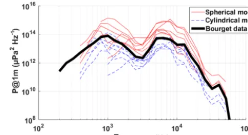
To measure the generated sound at different angles from the speaker, four hydrophones (HTI-96) were placed at a fixed distance of 0.7 m from the sound source (Fig. 1a). HTI-96 hydrophones have a flat frequency response between 2 Hz and 30 kHz (±2 dB), enabling absolute measurement of the acoustic power in this frequency range. The entire system was deployed in a lake with an aluminum structure to ensure the relative position of the sensors (Fig. 1b). To minimize the effect of this structure, all the sensors were attached to the structure with free ropes of 10 cm length. Several measure-ments of the emitted sounds were made by varying the depth of the system from 0.5 to 3.5 m and by changing the orien-tation of the loudspeaker (horizontal or vertical). The power spectral density (PSD) of each emitted chirp monitored by the four hydrophones has been computed and plotted all to-gether (Fig. 2). It can be observed that the generated sounds have a spectral power between 1012and 1014µPa2Hz−1but do not have a flat frequency response due to the transfer func-tion of the system. Overall, we observed that the monitored PSD was variable between the different tests that were con-ducted. The monitored power varied between±3 dB between the 25th and 75th quartiles, and between ±10 dB between the minimum and the maximum. The most important param-eter influencing the emitted sounds was the directivity of the loudspeaker (horizontal or vertical positions). The emitted signals also did not vary when repeating the same signal in a fixed configuration of emission.
This preliminary study indicated that we would not be able to precisely predict the power emitted by the sound source
during our experiments. The loudspeaker is deployed with a weighted rope from a bridge so that its orientation is uncer-tain when deployed on the riverbed. We therefore have an uncertainty concerning the initial power of the sound source (P@1 m) defined in the Eq. (1). This parameter will therefore be estimated for each experiment.
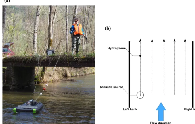
2.2 Hydrophone measurements at varying distances Acoustic measurements were performed with HTI-96 hy-drophones plugged to a EA-SDA14 recorder (RTSys com-pany). Acoustic signals were stored in wav files at a sam-pling frequency of 156 kHz. The acoustic recorder and the hydrophone are shared by a Carlson river board, drifting dur-ing the measurements (Fig. 3). Lagrangian measurements were preferred to fixed-position measurements to optimize the signal-to-noise ratio. By measuring when drifting, the noises generated by the resistance of the river board against the flow are drastically reduced. The hydrophone was located under the river board at a constant depth from the water sur-face. The underwater loudspeaker is deployed at a fixed po-sition on the river bed and emits a logarithmic chirp with an infinite loop of 1 s. During this time, several drift trajectories were made with the river board along the cross-section. As a first step, acoustic measurements were positioned using a synchronized GPS. This GPS equipment was damaged dur-ing the first field experiments requirdur-ing another way to po-sition the hydrophone during the drifts. The cross-sectional distance of the hydrophone was monitored at start positions and considered as constant during the drift (i.e., drifts are considered parallel to the river banks). Secondly, longitudi-nal positions of the hydrophone during the drift were com-puted knowing the start position and by assuming a constant velocity of the river board:
x(t)=x0
y(t)=y0+vdriftt, (6)
wherex andy are respectively the cross-sectional and lon-gitudinal positions of the hydrophone (m);x0andy0are the initial positions of the hydrophone monitored at the begin-ning of the drift;vdriftis the mean velocity of the river board during the drift (m s−1), computed as the traveled distance divided by the duration of the drift. The assumption of paral-lel drifts at a constant velocity was supported by the fact that our field sites are straight reaches.
Figure 1.(a)Schematic design of the test characterizing the system of emission;(b)photography of the immersed system in Lac du Bourget (France).
Figure 2.Power spectral densities (µPa2Hz−1) of the logarithmic chirps emitted by the loudspeaker.
2.3 Signal processing of the monitored acoustic waves The use of a matched filter was chosen to detect the chirps in the hydrophone signals. When a chirp is detected, the posi-tion of the measurement is computed by matching the time of detection with the position of the hydrophone. Finally, know-ing the position of the loudspeaker, the distance r, between the sound source and the measurement, is computed.
For each located chirp, a short-term spectrogram is com-puted using Hamming windows of 212points with 50 % over-lapping (Fig. 4). Based on this spectrogram, several PSDs are computed. First, the PSD of the studied chirp (noted PSDr) is computed by using the signal contained inside the black lines. The black lines correspond to the upper and lower lim-its of the octave band centered around the instantaneous fre-quency of the chirp. Secondly, the 95th percentile of the mon-itored power is computed (Merchant et al., 2013) in each fre-quency band. This PSD is used to represent the power of the ambient noise (PSD95). In this example (Fig. 4), one can par-ticularly observe the harmonics generated by the loudspeaker when reproducing the theoretical logarithmic chirp. The
am-bient noise depends on the sounds that are naturally gener-ated in the river (e.g., bedload impacts). To ensure that the chirp is not affected by ambient noise, we decided to keep only the chirps that are at least twice as powerful as the am-bient noise (i.e., PSDr>2 PSD95).
At this point, we can propose a protocol to monitor the PSD of an emitted chirp at varying distances from its point of emission.
2.4 Fitting propagation laws
The acoustic power of each chirp measured at a distancer was computed by integrating PSDrin third-octave bands. For thejth third-octave band,Pi,j is the acoustic power of the
ith measurement made at a distanceri from the loudspeaker.
Using the theoretical model (Eq. 4) and assuming one model of geometric spreading loss (cylindric or spherical), the esti-mated acoustic powerPgi,j as a function ofriis
g
Pi,j =P@1 m,jG(ri)e−2∝jri, (7)
whereP@1 m,j andαj are parameters to fit for each
third-octave bandj. These parameters were estimated with a non-linear least-square algorithm on the log values of power. It means that P@1 m,j andαj were estimated by minimizing
the following term:
N
P
i=1
log(gPi,j)−log(Pi,j)
2
, whereN is
the total number of observed chirps.
For each frequency band, the fit was characterized by a coefficient of correlation between the log values of the es-timated power (gPi,j) and the log values of the measured
power (Pi,j). Finally, the residuals (dB) of the fits were
com-puted using the following relationship: N1
N
P
i=1 10 log(
g
Pi,j
Pi,j)
.
The residuals are the average variation of the data set around the fitted law, it represents the dispersion of the data set.
consider-Figure 3.(a)Drifting board sharing the hydrophone and the acoustic recorder.(b)Drift trajectories of the recorder during the measurements.
Figure 4.Short-term spectrogram of a chirp monitored by a hy-drophone in the Leysse River. The black lines indicate the octave band centered around the instantaneous frequency of the theoretical logarithmic chirp.
ing third-octave bands, therefore enabling the estimation of P@1 mandαin several frequency bands. Note that these esti-mations were done by considering either a cylindrical (Eq. 2) or spherical model (Eq. 3).
2.5 Field sites
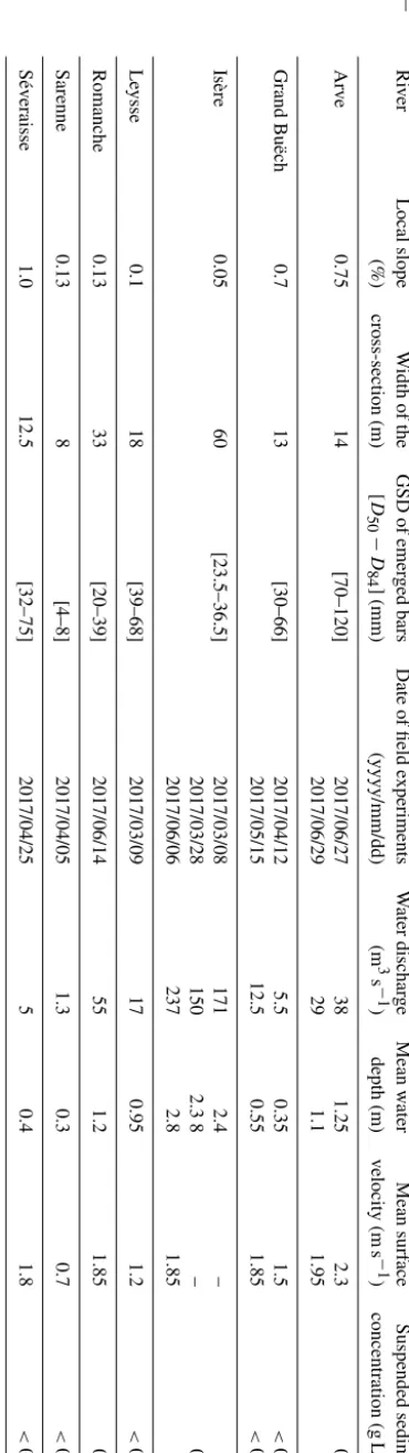
The protocol presented in the previous section was applied in seven field sites located in the French Alps. Their charac-teristics are presented in Table 1. The mean bed slope of the studied reaches varies from 0.05 % to 1 %, and the width of the cross-section from 8 to 60 m. The roughness (or the sur-face particle size distribution) of the river bed is a difficult
parameter to measure, particularly in rivers that are not wad-able. This aspect of bed roughness was approached by do-ing Wolman measurements on the closest emerged bars. The surfaceD84of emerged bars varies from 20 to 150 mm. Hy-draulic parameters (discharge, surface velocity and mean wa-ter depth) were obtained by using several methods (acoustic Doppler current profiler, surface velocity radar (SVR) gun or existing gauging station) depending on the field sites. Finally, the measurement of suspended sediment load was achieved with a turbidimeter (Visoturb, WTW).
3 Results
3.1 The Leysse River
T ab le 1. Field site characteristics. GSD is grain size distrib ution. Ri v er Local slope W idt h of the GSD of emer ged bars Date of field experiments W ater dischar ge Mean w ater Mean surf ace Suspended sediment (%) cross-section (m) [ D 50 − D 84 ] (mm) (yyyy/mm/dd) (m 3 s− 1 ) depth (m) v elocity (m s− 1 ) concentration (g L − 1 ) Arv e 0.75 14 [70–120] 2017/06/27 38 1.25 2.3 0.35 2017/06/29 29 1.1 1.95 – Grand Buëch 0.7 13 [30–66] 2017/04/12 5.5 0.35 1.5 < 0 . 05 2017/05/15 12.5 0.55 1.85 < 0 . 05 Isère 0.05 60 [23.5–36.5] 2017/03/08 171 2.4 – 0.1 2017/03/28 150 2.3 8 – 0.06 2017/06/06 237 2.8 1.85 0.6 Le ysse 0.1 18 [39–68] 2017/03/09 17 0.95 1.2 < 0 . 05 Romanche 0.13 33 [20–39] 2017/06/14 55 1.2 1.85 0.14 Sarenne 0.13 8 [4–8] 2017/04/05 1.3 0.3 0.7 < 0 . 05 Sév eraisse 1.0 12.5 [32–75] 2017/04/25 5 0.4 1.8 < 0 . 05
Figure 5.Data from the Leysse River. Measured acoustic power (µPa2) as a function of the distance between the hydrophone and the active source. Results obtained in the third-octave band centered on 1 kHz. Spherical and cylindrical fits are in thick lines. Fits and data sets are presented for other frequencies in the Supplement.
Results of the fits are shown in Fig. 6 for the Leysse River experiment. Logically, attenuation coefficients that are es-timated with cylindrical spreading loss exhibit higher val-ues than coefficients estimated with spherical spreading loss. However, they behave similarly with frequency variations. At low frequency, approximatively below 103Hz, the attenu-ation coefficient is higher. This result was expected because of the existence of a cutoff frequency (Geay et al., 2017b). The cutoff frequency is dependent on the water depth (mean water depth of 0.95 m), the sound speed in water (assumed to be equal to 1500 m s−1) and the sound speed in the sediment layer. Typical values of sound speed in sea floor materials (from silt to gravel) were observed to vary between 1550 and 2000 m s−1 (Jensen et al., 2011), depending on many factors such as the type of materials, grain sizes or porosity (Hamilton and Bachman, 1982). Using sound speed of 1550 and 2000 m s−1in the sediment leads to cutoff frequencies of 1500 and 600 Hz, respectively, which is consistent with our observation.
Above 103Hz, attenuation coefficient increases with quency: acoustic waves are more attenuated at higher fre-quencies. Considering the estimation of the sound source power, it is observed that the cylindrical model best repro-duces the power monitored in the experiment made in Lac du Bourget (the median value is represented in Fig. 6b). Using a spherical model, we overestimate the power of the sound source by approximatively 1 order of magnitude. However, as we will see for other experiments, the best estimation of the sound source power is sometimes obtained with spherical spreading loss model.
Figure 6.Data obtained for the Leysse River(a)attenuation coeffi-cient (nepers m−1);(b)sound source power spectral density (P@1 m in µPa2Hz−1) estimated with spherical/cylindrical models. Data from Lac du Bourget are the median values of the measurement presented in Fig. 2;(c)residuals of the regression (dB);(d)squared correlation coefficient of the fits.
mean square difference between data and fits. In the Leysse River, we observed that the power of the reception fluctuates between 2 and 3 dB around the fits.
Finally, considering the correlation coefficients of the fit-ted laws (Fig. 6d), we cannot make a distinction between spherical or cylindrical spreading loss models.
3.2 Propagation laws in several rivers
Propagation properties of several rivers were investigated. For some of the rivers, experiments were done at different hydrodynamic conditions (Table 1). For the discharge inves-tigated, hydrodynamic conditions were not variable enough to observe major differences in the results. We therefore de-cided to gather data to propose a unique result for each river. The data set is presented in the Supplement, for all rivers and for different frequency bands. A first result concerns the es-timated power of the sound source (P@1 m) emitted during the experiments (Fig. 7). Compared with the measurements made in Lac du Bourget, it can be observed that the estima-tion of the sound source power is overestimated when using a spherical model and underestimated when using a cylindrical model of the geometric spreading loss. Considering the cor-relation coefficients of the data to the fits, we did not observe a significant difference between the models. Based on these observations, we are not able to argue that geometric spread-ing is cylindrical or spherical in these rivers. In the follow-ing, all the results are presented by assuming a cylindrical, spreading loss model.
The attenuation coefficients obtained for each river are presented as a function of frequency (Fig. 8). From the Isère to the Arve river, we can observe that the attenuation coef-ficient varies by more than 1 order of magnitude (Fig. 8b).
Figure 7.Power spectral density of the source power (P@1 m in µPa2Hz−1) estimated with spherical and cylindrical models for all experiments made in rivers and measured in Lac du Bourget.
Looking at the linear representation (Fig. 8a), we see that the variation of the attenuation coefficient with frequency is different from case to case. It increases faster for rivers hav-ing the largest attenuation coefficients. Note that minimal and maximum frequencies of the observations are variable from one river to another. At low frequency, observations are lim-ited by the cutoff frequency which is inversely proportional to the water depth (Geay et al., 2017b). At high frequencies, measurements are limited by too-strong attenuation of the emitted acoustic waves.
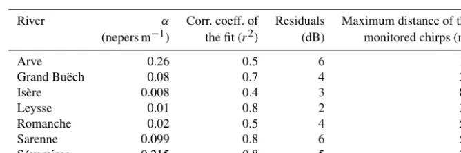
Table 2 contains, for each river, a summary of the results obtained by fitting a cylindrical propagation model to the data. All the parameters indicated in this table are an av-erage of the values obtained between 1 and 10 kHz. It can be observed that the correlation coefficients vary from 0.4 to 0.8. We observed that the lowest correlation coefficients were obtained for the largest rivers (Isère and Romanche rivers with section widths of 60 and 33 m, respectively) and may be representative of cross-sectional variations that have not been considered in this study. The residuals vary from 2 to 6 dB. Rivers having largest attenuation coefficients seem to have larger residuals: the dispersion of the monitored acous-tic power is larger when the attenuation is larger. Finally, the maximum distance of the monitored chirps represents the maximum distance from the hydrophone to the underwater speaker where we were able to record the chirps with a suffi-cient signal-to-noise ratio. The smaller the attenuation coef-ficient, the larger the maximum distance of the observation. Note that the maximum distance is also dependent on opera-tional issues.
4 Discussion
4.1 Attenuation processes in rivers
Figure 8.Attenuation coefficient (αin nepers m−1) obtained when using a cylindrical model of the geometrical spreading loss:(a)linear and(b)logarithmic scales. Black symbols indicate the cutoff frequency computed with Eq. (8), sound speeds of 1500 and 1600 m s−1in the water and sediment layer, respectively.
Table 2.Average results over frequency (1–10 kHz) of the parameters of the fit using cylindrical geometrical spreading.
River α Corr. coeff. of Residuals Maximum distance of the (nepers m−1) the fit (r2) (dB) monitored chirps (m)
Arve 0.26 0.5 6 11
Grand Buëch 0.08 0.7 4 31
Isère 0.008 0.4 3 80
Leysse 0.01 0.8 2 39
Romanche 0.02 0.5 4 59
Sarenne 0.099 0.8 6 57
Séveraisse 0.215 0.8 5 22
10−3 nepers m−1from 1 to 100 kHz (Fisher and Simmons, 1977). The attenuation due to water only does not explain the coefficients of attenuation that were found in this study. In this section, we wonder how propagation properties are re-lated to typical characteristics of the rivers (e.g., slope, water depth). As shown in Fig. 8, the dependency of the attenuation coefficient to frequency does not follow a simple law.
At low frequency, around 1 kHz, acoustic wave propaga-tion should be affected by wave guide properties. The river could be considered as an acoustic wave guide where sounds are partly trapped between the water surface and the river bed (Geay et al., 2017b): this problem is known as the Pekeris wave guide. Theoretically, in a perfect medium without atten-uation, it can be shown that acoustic waves having frequen-cies lower than the cutoff frequency are exponentially decay-ing with horizontal distance (Jensen et al., 2011). The cutoff frequencyfcutoff(Hz) is dependent on the wave guide charac-teristics, water depth and sediment layer acoustic properties, as shown in the following equation:
fcutoff=
cscw 4hpc2
s−c2w
, (8)
wherehis the water depth (m),cs andcware sound celerity (m s−1) in the sediment layer and in water, respectively. Cut-off frequencies have been estimated in each river, by assum-ing a fixed sound speed of 1600 m s−1in the sediment layer
and using the mean water depth monitored (Fig. 8b). Esti-mated cutoff frequencies are approximatively located around the minimum of the observed attenuation coefficient. Our ability to precisely determine a cutoff frequency is limited. First, the acoustical properties of river beds are unknown, depending on lithology, grain sizes, porosity and heterogene-ity of the materials constituting the river bed. Secondly, the water depth is not constant over the investigated sections but varies from the banks to the middle of the river. For these rea-sons, cutoff frequencies are rough estimates and do not per-fectly correspond to the observed local minimum of attenua-tion coefficient. Note also that different hydrodynamic condi-tions were investigated for some rivers. Varying water depth results in different cutoff frequencies and relative positions of the hydrophone between water surface and streambed. These two parameters have been observed to modify the response of the hydrophone (Geay et al., 2017b) in the lower frequency range, around the cutoff frequency. The range of hydrody-namic conditions that was investigated in this study did not enable the observation of such effects.
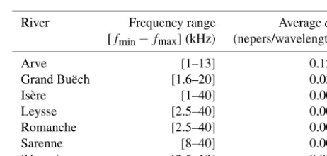
wavelength (nepers) are presented in Fig. 9 for frequencies higher than the local minimum of α (nepers m−1). Except for the Isère river, we can observe thatαλis almost constant
with frequency, which in turns means that α (nepers m−1) varies almost linearly with frequency. Note that the maxi-mum frequency analyzed in Fig. 9 varies from one river to another and shows some inverse correlation with the aver-ageαλ. In rivers with high attenuation (highαλ), the
record-ing of the emitted chirps was not possible in the highest frequency range, due to a too-fast decrease of chirp power with distance. This observation reveals that the measurement of bedload sounds generated by the smallest particles (i.e., highest frequencies generated) should be local or even im-possible in rivers having too-high attenuation coefficients. In the following, each river is characterized by an average value ofαλ (Table 3) and is compared to river
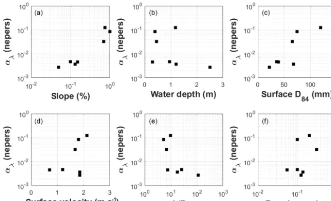
characteris-tics (Table 1; Fig. 10). Looking at the relationship between αλ and the slope measured at the local reach (i.e., 100 m
downstream and upstream from the bridge where experi-ments were undertaken), we can observe that there is good correlation: higher attenuation coefficients were obtained for steeper rivers. As for slope, surficial granulometry of the emerged bars (D84) is also well correlated with αλ: larger
roughness (i.e., largerD84) induces larger attenuation of the acoustic waves. Surface velocity or water depth seems to be a less robust explanatory variable ofαλ. The possible
influ-ence of typical nondimensional numbers has also been tested. The ratio of the water depth overD84 and the Froude num-ber were used by Tonolla et al. (2009, 2010). They found that they were the main hydrogeomorphological variables plaining the differences in passive acoustic signals in field ex-periments. Small ratio of the relative submergence (i.e., small h/D84) induces breaking waves or water plunging directly in the water column, entraining bubbles in the water column. These hydraulic mechanisms are sources of noise generated by oscillating air bubbles in the water column, as it is ob-served for breaking waves in a marine environment (Deane, 1997; Norton and Novarini, 2001). In our study, entrained air bubbles could explain the increase of attenuation coeffi-cient in rivers having rough beds. It is indeed known that the presence of air bubbles increases the attenuation of acoustic waves (Deane, 1997; Norton and Novarini, 2001) because of the heterogeneity of the medium constitution of water and air which have very different acoustic impedances. Also, as observed in a flume experiment (Wren et al., 2015), the bed roughness itself is a source of attenuation, with larger rough-ness involving higher attenuation. Finally, both processes (rough boundaries and entrained air bubbles) could explain our observations by causing concomitantly higher attenua-tion of the acoustic wave. The river bed roughness should be the best characteristic enabling the prediction of acoustic wave propagation properties in rivers. However, this param-eter is not easy to measure. It is sometimes difficult to access the riverbed, and surface grain size distributions are known to be variable in space. The local slope of the reaches is
eas-Figure 9.Attenuation coefficient per wavelength (nepers) as a func-tion of frequency (Hz) above the cutoff frequency.
Table 3.Frequency bands whereαλ was observed to be almost
constant with frequency and average values ofαλin this frequency
range.
River Frequency range Averageαλ
[fmin−fmax] (kHz) (nepers/wavelength)
Arve [1–13] 0.125
Grand Buëch [1.6–20] 0.032
Isère [1–40] 0.003
Leysse [2.5–40] 0.005
Romanche [2.5–40] 0.004
Sarenne [8–40] 0.005
Séveraisse [2.5–13] 0.085
ier to measure and, even if less meaningful, should be a more robust parameter to infer propagation properties of a river.
4.2 Recommendation for monitoring bedload with hydrophones
This study was done to improve our ability to better use the measurements of bedload self-generated noise in rivers. This section aims at giving an example on the use of attenua-tion coefficients in a simple case. Let us consider an infinite river bed with a homogeneous repartition of sound sources over the river bed. Bedload impacts generate a constant spec-tral power per surface unit noted PSDs (µPa2Hz−1m−2). If sound sources are random and independent noise sources (Thorne, 2014), the acoustic power measured by a hy-drophone can be written as a sum of the power of all sound sources:
PSDh(f)= ∞ Z
d
2PSDs(f) rh e
−2α(f)r2π rdr, (9)
Figure 10.Representation of the attenuation coefficient per wavelength (αλin nepers) as a function of river characteristics:(a)local slope
(%);(b)average water depth (m);(c)surfaceD84(mm) of the closest emerged bars;(d)average surface velocity (m s−1);(e)ratio of water depth (m) over surfaceD84(m);(f)Froude number computed with average flow velocity (m s−1) and water depth (m).
(m). From Eq. (9), it follows that
PSDh(f)=
2πPSDs(f) hα(f) e
−2α(f)d. (10)
Considering that 0< α1, it follows that PSDh is in-versely proportional to the attenuation coefficient as the ex-ponential term tends to 1. This has several implications for the use of bedload monitoring using passive acoustics. First, as the attenuation coefficient could be variable from one reach to another, the acoustic power of bedload SGN could be variable from one reach to another even if bedload fluxes are similar. Secondly, as observed in Fig. 8, attenuation co-efficients are variable with frequency. It means that the fre-quency content of bedload SGN spectra is modified by prop-agation effects, which in turns means that the shape of mon-itored spectra is not only related to grain size distributions (Petrut et al., 2018; Thorne, 2014) but also to propagation properties. Therefore, in order to estimate grain size distri-bution, measured spectra should be corrected for propaga-tion effects before any inversion procedure. From Eq. (10) (α1), a better estimate of the sound generated by bedload transport could be done by multiplying the monitored sound pressure levels by the attenuation coefficient (α >0):
PSDs(f)= h
2πα(f)PSDh(f). (11)
The power generated by bedload sounds is proportional to the power of measured sounds multiplied by the attenua-tion coefficient. This simple operaattenua-tion enables us to get an unbiased measurement of the sound generated by bedload impacts and therefore a more robust proxy for bedload trans-port monitoring in rivers. To achieve the estimation of sounds
that are generated by bedload transport (PSDs), both mea-surements of propagation properties (α) and ambient sounds (PSDh) are needed. Note that Eq. (11) was obtained by as-suming sound sources (i.e., bedload fluxes) that are homoge-neously distributed. As this hypothesis will rarely be valid, more realistic inverse methods should be invented to estimate the real sounds (PSDs) generated by bedload transport and its spatial distribution.
5 Conclusions
local minimum (i.e., the cutoff frequency), attenuation coef-ficients increase almost linearly with frequency. The higher frequency regime has been characterized by a constant at-tenuation coefficient per wavelength (αλ in nepers). It has
been found thatαλwas well correlated with the slope of the
riverbed reaches (and to the surfaceD84of the emerged bars as well), whereαλis higher for higher bed slopes of the river.
Assuming that riverbed slope and surface D84 of bars are good proxies for the riverbed texture, it can be concluded that attenuation properties are dominated by processes re-lated to the riverbed roughness at high frequencies, includ-ing the entrainment of air bubbles in the water column and scattering effects on rough boundaries. As shown in the dis-cussion, the acoustic power monitored by a hydrophone, in a fixed position, is almost inversely proportional to the attenu-ation coefficient at a given frequency. As consequences, the spectra of bedload SGN that are measured in rivers are mod-ified by the variations of attenuation coefficients with fre-quency. As attenuation is higher at high frequencies, acous-tic signals that are monitored by a hydrophone are shifted to lower frequencies compared to the sound really generated by bedload impacts. As shown for an idealized case with an infinite riverbed and homogeneous bedload sound sources, the real sounds generated by bedload can be estimated by correcting the hydrophone signal by the propagation laws of acoustic waves in rivers.
Data availability. Data supporting the content of this paper can be obtained by contacting Electricité de France ([email protected]).
Supplement. The supplement related to this article is available online at: https://doi.org/10.5194/esurf-7-537-2019-supplement.
Author contributions. TG developed the signal processing tools and prepared the manuscript with contributions from all co-authors. TG, LM and SZ designed and carried out he experiments. JRR helped in designing the experiments thanks to previous experience and was integral in the analysis of the results.
Competing interests. The authors declare that they have no con-flict of interest.
Acknowledgements. The authors are grateful to all the contribu-tors to this work; particularly abundant during field experiments was Guy Cellier (EDF), who designed the equipment to record sounds with a river board. This work has also been carried out with the help of engineering consultants and numerous students.
Financial support. This project was essentially founded by Eléc-tricité de France with additional subsidy from Agence de l’eau Rhone-Alpes, the Rhone-Alpes region (ARC3-Environment) and Grenoble University (OSUG).
Review statement. This paper was edited by Jens Turowski and reviewed by two anonymous referees.
References
Barton, J., Slingerland, R. R. L., Pittman, S., and Gabrielson, T. B.: Monitoring coarse bedload transport with passive acoustic instrumentation: A field study, US Geol. Surv. Sci. Investig. Rep. 2010–5091, 38–51, 2010.
Deane, G. B.: Sound generation and air entrainment by break-ing waves in the surf zone, J. Acoust. Soc. Am., 102, 2671, https://doi.org/10.1121/1.420321, 1997.
Fisher, F. H. and Simmons, V. P.: Sound absorption in sea water, J. Acoust. Soc. Am., 62, 558–564, https://doi.org/10.1121/1.381574, 1977.
Geay, T., Belleudy, P., Gervaise, C., Habersack, H., Aigner, J., Kreisler, A., Seitz, H., and Laronne, J. B.: Pas-sive acoustic monitoring of bed load discharge in a large gravel bed river, J. Geophys. Res.-Earth, 21, 2010, https://doi.org/10.1002/2016JF004112, 2017a.
Geay, T., Belleudy, P., Laronne, J. B., Camenen, B., and Gervaise, C.: Spectral variations of underwater river sounds, Earth Surf. Proc. Land., 42, 2447–2456, https://doi.org/10.1002/esp.4208, 2017b.
Gray, J. R., Laronne, J. B., and Marr, J. D. G.: Bedload-Surrogate Monitoring Technologies Scientific Investigations Report 2010, 37 pp., 2010.
Hamilton, E. L. and Bachman, R. T.: Sound velocity and related properties of marine sediments, J. Acoust. Soc. Am., 72, 1891– 1904, https://doi.org/10.1121/1.388539, 1982.
Jensen, F. B., Kuperman, W. A., Porter, M. B., and Schmidt, H.: Computational Ocean Acoustics, edited by: Springer Sci-ence & Business Media, ISBN 1441986782, 9781441986788 https://doi.org/10.1007/978-1-4419-8678-8, 2011.
Johnson, P. and Muir, T. C.: Acoustic Detection Of Sediment Movement, J. Hydraul. Res., 7, 519–540, https://doi.org/10.1080/00221686909500283, 1969.
Jonys, C. K.: Acoustic Measurement of Sediment Transport, Sci. Ser., 66, ISBN 0662004744, 9780662004745, 1976.
Lugli, M. and Fine, M. L.: Stream ambient noise, spectrum and propagation of sounds in the goby Padogobius martensii: Sound pressure and particle velocity, J. Acoust. Soc. Am., 122, 2881, https://doi.org/10.1121/1.2783113, 2007.
Marineau, M. D., Wright, S. A., and Gaeuman, D.: Calibration of sediment-generated noise measured using hydrophones to bed-load transport in the Trinity River, California, USA, Proc. River Flow Conf., 1519–1526, 2016.
Medwin, H.: Sounds in the Sea: From Ocean Acoustics to Acoustical Oceanography, Cambridge Univ. Press., 643, ISBN 052182950X, 9780521829502, 2005.
for ambient noise analysis, J. Acoust. Soc. Am., 133, EL262-7, https://doi.org/10.1121/1.4794934, 2013.
Norton, G. V. and Novarini, J. C.: On the relative role of sea-surface roughness and bubble plumes in shallow-water propaga-tion in the low-kilohertz region, J. Acoust. Soc. Am., 110, 2946, https://doi.org/10.1121/1.1414883, 2001.
Petrut, T., Geay, T., Gervaise, C., Belleudy, P., and Zanker, S.: Pas-sive acoustic measurement of bedload grain size distribution us-ing self-generated noise, Hydrol. Earth Syst. Sci., 22, 767–787, https://doi.org/10.5194/hess-22-767-2018, 2018.
Richards, S. D., Heathershaw, A. D., and Thorne, P. D.: The effect of suspended particulate matter on sound attenuation in seawater, J. Acoust. Soc. Am., 100, 1447, https://doi.org/10.1121/1.415991, 1996.
Rigby, J. R., Wren, D., and Murray, N.: Acoustic signal propagation and measurement in natural stream channels for application to surrogate bed load measurements: Halfmoon Creek, Colorado, River Flow Conf., 1566–1570, 2016a.
Rigby, J. R., Wren, D. G., and Kuhnle, R. A.: Passive Acoustic Monitoring of Bed Load for Fluvial Applications, J. Hydraul. Eng., 142, 02516003, https://doi.org/10.1061/(ASCE)HY.1943-7900.0001122, 2016b.
Thorne, P. D.: An overview of underwater sound generated by in-terparticle collisions and its application to the measurements of coarse sediment bedload transport, Earth Surf. Dynam., 2, 531– 543, https://doi.org/10.5194/esurf-2-531-2014, 2014.
Tonolla, D., Lorang, M. S., Heutschi, K., and Tockner, K.: A flume experiment to examine underwater sound generation by flowing water, Aquat. Sci., 71, 449–462, https://doi.org/10.1007/s00027-009-0111-5, 2009.
Tonolla, D., Acuña, V., Lorang, M. S., Heutschi, K., and Tockner, K.: A field-based investigation to examine underwater sound-scapes of five common river habitats, Hydrol. Process., 24, 3146– 3156, https://doi.org/10.1002/hyp.7730, 2010.
Turowski, J. M. and Rickenmann, D.: Tools and cover effects in bedload transport observations in the Pitzbach, Austria, Earth Surf. Proc. Land., 34, 26–37, https://doi.org/10.1002/esp.1686, 2009.