Construction of Quick Switching Variables Sampling System Indexed by Crossover Point

(1)

Construction of Quick Switching Variables

Sampling System Indexed by Crossover

Point

Dr. D. SENTHILKUMAR1* SR. SATHYA MOHAN RAJ2 B. ESHA RAFFIE2

1

Associate Professor, Department of Statistics, PSG College of Arts & Science, Coimbatore -641 014

2

Research Scholar, Department of Statistics, PSG College of Arts & Science, Coimbatore -641 014

Abstract

The Quick Switching Sampling System by attributes was devised by Romboski(1969). He has studied a new system, comprising normal and tightened plans, called a Quick Switching System (n;cT,cN) [(n,cN) and

(n,cT) are normal and tightened single sampling plans, respectively, with cT<cN], proposed by Dodge (1967).

In this Paper, Designing Quick Switching Variables Sampling System [QSVSS (n; kN, kT)] indexed by

Crossover Point is presented. The method of designing the plan based on the given pc and hc is provided. Table

yielding plans for given set of entry parameters namely pc, Crossover Point and hc.

Keyword: Quick Switching Sampling System, Variable Sampling Plan, OC Function, Crossover Point and Relative Slope

1. Introduction

Dodge (1967) has proposed a new type of sampling plan namely Quick Switching Sampling System and investigated by Romboski (1969), Govindaraju (1991), Deveraj Arumainayagam (1991) and Taylor (1992). Romboski introduced QSS-1 (n;cN,cT) which is a QSS-1 with single sampling plan as a reference plan [(n,cN),

(n,cT) are respectively the normal and tightened single sampling plans with cT<cN]. Palanivel(1999) has studied

the contributions to the study of designing of Quick Switching Variables System and Devaraj Arumainayagam and Soundararajan (1996) introduced a new designing methodology for Quick Switching attribute sampling schemes, indexed by an entry parameter called the Crossover Point (COP). The significance of the COP and the properties of the Operating Characteristic (OC) with respect to it are studied and the necessary tables constructed. .

In this paper, Quick Switching Variables Sampling System [QSVSS(nσ;kN,kT)] is considered and

procedure and table are developed for the selection of the scheme, indexed by a new criterion called the Crossover Point.

2. QSS Variables Sampling System of type QSVSS (n;kN,kT)

The conditions and the assumptions under which the QSVSS scheme can be applied are as follows:

2.1 Conditions for application

• Production is steady so that results on current, preceding and succeeding lots are broadly indicative of a continuing process.

• Lots are submitted substantially in the order of production. • Normally lots are expected to be essentially of the same quality.

• Inspection is by variables, with quality defined as the fraction non-conforming.

2.2 Basic Assumptions

• The quality characteristic is represented by a random variable X measurable on a continuous scale. • Distribution of X is normal with mean and Standard deviation.

• An upper limit U, has been specified and a product is qualified as defective when X>U. [when the lower limit L is Specified, the product is a defective one if X<L].

(2)

When the conditions listed above are satisfied the fraction defective in a lot will be defined by

p = 1-F (v) = F (-v) with v = (U-μ) /σ and

F(y) =



∞ −

− 1

2 _/ ₂

2

1

y

z

dz

e

π

(1)

Where z ~ N (0, 1). It is to be recalled here that the criterion for the σ -method variable plan is to accept the lot if

x

+ kTσ ≤ U, where U is the upper specification limit or

x

+ kTσ ≥ L, where L is the lower

specification limit. The operating procedure of QSVSS (n;kN,kT) is described below.

3. Operating Procedure

The steps involved in this procedure is as follows

(i) Take the sample size nσ from the population. Inspect each unit and record the measurement of the

quality characteristic of the sample. Compute the sample mean

x

.

(ii) If

x

+ kNσ≤ U or

x

+ k Nσ ≥ L accept the lot and repeat step 1 otherwise go to step 3.

(iii) Take a sample of size nσ from the next lot and inspect each unit and record the measurement of the

x

.

(iv) If

x

+ kTσ≤ U or

x

+ kTσ ≥L accept the lot and go to step 1 otherwise repeat step 3.

where kN and kT are the acceptance criterion. Where

x

and σ are the average quality characteristic

and standard deviation respectively derived from the population.

4. Operating Characteristic Function

According to Romboski (1969), the OC function of COP for QSS is given by

Pa(pc) =

2

1

(PN + PT) (2)

Based on the OC function of the QSS Romboski (1969) the OC function of QSVSS (n_σ;kN,kT) can be

written as

Pa (p) =

)

(

)

(

1 )

(

T N

T

w

ϕ

+

−

(3)

with

_w

T =

n

σ (U-kT-μ)/σ = (v-kT)

n

σ w_N =

n

_σ (U-kN-μ)/σ = (v-kN)

n

_σ

v = (U-μ) /σ

Under the assumption of normal approximation to the non-central t distribution (Abramowitz and Stegun, 1964), the values of PN and PT are respectively given by

PN = F (wN) = Pr [(U-

x

)/σ>kN] (4)

PT = F (wT) = Pr [(U-

x

)/σ < kT] (5)

Where, PN and PT are the proportions of lots expected to be accepted using normal (nσ,kN) and tightened

(n_σ,kT) variable single sampling plans respectively. These two equations are applied in the OC function of QSS

(n;cN,cT). We get the following

Pr [(U-

x

)/σ> kT]

Pa (p) = (6)

1- Pr [(U-

x

)/σ> kN] + Pr [(U-

x

)/σ> kT]

The relative slope at pc, known as “hc”, is used to measure the discriminating power of the OC curve. In

symbolic terms, the hc of QSVSS (nσ;kNσ,kTσ) is such that

hc = a

a

dP (p)

p

(3)

where,

dP (p)

a

dp

=

N T T T N T

2

N T

(1-P +P )P +P (P -P )

(1-P +P )

′

′ ′

at p = pc

in which

PT(p) =



∞ −

−

Τ

w

z

dz

e

2 /2

2

1 π

and PN(p) =



∞ −

−

N

w

z

dz

e

2/2

2

1 π

with wT = (v-kT)

n

and wN = (v-kN)

n

and

P (p)= n exp(v -w )

T

′

2 T2

P (p)= n exp(v -w )

_N

′

2 2_N

5. Designing QSVSS (nσ;kN,kT) System for given pc and hc

From table 1, a method of designing of Quick Switching Variables Sampling System for the given values of COP is indicated below.

Table 1 fixes the COP (pc) and the relative slope at this point (hc) from which a Quick Switching

Variables Sampling System can be selected under known σ-method. Entering the row giving pc and hc, one gets

the acceptance criteria kT and kN and the sample size nσ of QSVSS (nσ;kNσ,kTσ). For example, for given pc=.005,

hc=2.00, nσ=49, kTσ=2.58507, kNσ=2.57407.

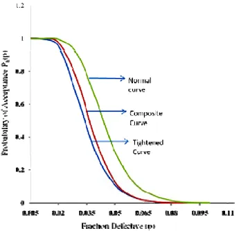
5.1 Plotting the OC Curve

The OC curve for the Quick switching sampling system by variables with n=56 ;

kT =1.793 & kN = 1.706 and Fig 1 shows the OC curve of Quick Switching Sampling system by variables

(4)

Figure 1. Normal, Composite and Tightened OC Curves with CrossOver Point for QSVSS, (n=56 kT =1.793 & kN

=1.706)

6. QSVSS with unknown σ variable plan as the reference plan

If the population standard deviation σ is unknown, then it is estimated from the sample standard deviation s (n-1 as the divisor). If the sample sizes of the unknown sigma variables system (s method) are ns and

cns the acceptance parameter is k0, then the operating procedure is as follows:

1) Take the sample size nS from the population. Inspect each unit and record the measurement of the

x

.

2) If

x

+ kNS ≤ U or

x

+ kN S≥ L accept the lot and repeat step 1 otherwise go to step 3.

3) Take a sample of size nS from the next lot and inspect each unit and record the measurement of the

x

.

4) If

x

+ kTS ≤ U or

x

+ kTS ≥L accept the lot and go to step 1 otherwise repeat step 3.

Here

x

and s are the average and the standard deviation of quality characteristic respectively from the sample. Under the assumptions for Quick Switching System stated, the probability of acceptance Pa (p), of a lot

is given in the equation (3) and PT and PN respectively are

PT = Τ

2 W

- z / 2

-1

e

d z

2 π

∞



and PN = N

2

W

- z / 2

-1

e

d z

2 π

∞



with wN =

s

2 N

s s

U-k -

μ

1 .

s

₁

_k

+

n

2n













(5)

wT =

s

2 T

s s

U-k -

μ

1 .

s

₁

_k

+

n

2n













7. Designing QSVSS (nS;kN,kT) System with unknown σ for given pc and hc

Table 1 can be used to determine QSVSS (ns;kT,kN) for specified values of pc and hc. For example, if it is

desired to have a QSVSS (ns;kTS,kNS) for given pc= .005, hc=2.00 ,Table 1 gives ns=212,kTS=2.58814,

kNS=2.57712 as desired plan parameters.

8. Construction of Table

The OC function of QSVSS (n; kT, kN) is given by equation (2). For specified pc and hc the equation (7) would

result in T a c N T

P

P (P )

1 -P + P

=

(8)

where,

T

2

w

- z / 2 T

-1

P

=

e

d z

2 π

∞



(9)

and

N

2

w

- z / 2 N

-1

P

=

e

d z

2 π

∞



(10)

By substituting the equation (9) and (10) into (8), one can get the OC function of the QSVSS (nσ;kT,

kN). For given various values of pc and hc, the values of n, kT, kN are obtained by using computer search routine.

The values of n, kT, kN for the QSVSS that satisfying equation (2) are obtained using (8). By definition, the

relative slope Pa(pc) at p=pc is determined as

a c

a p = p_c

dP (p )

-p

h =

P (p)

dp

A procedure for finding parameters of S- method scheme from σ – method scheme with parameters (ns;kT, kN) were derived using Hamaker (1979) approximation as follows:

ns = nσ(1+

k

_σ2/2), where kσ = (kTσ + kNσ)/2

kTs = kTσ(4ns – 4)/(4ns – 5) and kNs = kNσ(4ns – 4)/(4ns – 5)

Table 1 provides the values of nσ, kTσ, kNσ, ns, kTs and kNs which satisfy equation (8),(9) and (10).

9. Conclusion

In this work, a new quality index called the crossover point has been introduced to the common quality indices for the design of the Quick Switching variables sampling system. By specifying values of COP, it is possible to control the application of normal and tightened plans in the Quick Switching (n;kT,kN) system, to get

enhanced system with regard to smaller sample size and the OC curve.

Reference

[1] M. Abramowitz, and I.A. Stegun,. Handbook of Mathematical Functions. National Bureau of Standards, Applied Mathematical Series No.55, 1964.

[2] S. Devaraj Arumainayagam. Contributions to the study of Quick Switching System (QSS) and its Applications. Doctoral Dissertation, Bharathiar University, Coimbatore, Tamil Nadu, India, 1991.

[3] S. Devaraj Arumainayagam, and V. Soundararajan. Sampling System indexed by the crossover point: Quick Switching System Indexed by a parameter called ‘COP’. Journal of Applied Statistics, Vol.23, No.1, pp. 115-123,1996.

[4] H.F. Dodge. A New Dual System of Acceptance Sampling Technical Report No. 16, The Statistics Center, Rutgers –The State University, New Brunswick, NJ, 1967.

[5] K. Govindaraju. Procedures and Tables for the selection of Zero Acceptance Number Quick Switching System for Compliance Testing. Communications in Statistics-Simulation and Computation, vol.20, No. 1, pp. 157-172, 1991.

[6] H.C. Hamaker. Acceptance Sampling for Percent Defective and by Attributes, Journal of Quality Technology, 11, pp.138-148, 1979. [7] M. Palanivel. Contributions to the Study of Designing of Quick Switching Variable System and Other Plans, PhD thesis, Bharathiar

University, 1999.

(6)

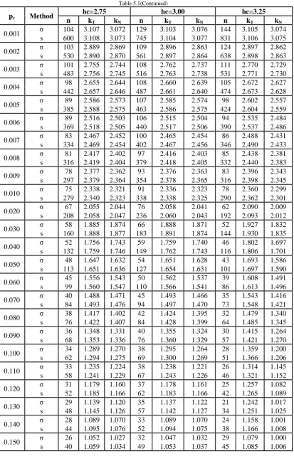
Table 1 The Value of nσ, kTσ, kNσ, ns, kTs, kNs for given pc and hc for QSVSS(n;kT,kN) indexed by Cross-Over Point

Pc Method hc=0.50 hc=0.75 hc=1.00

n kT kN n kT kN n kT kN

0.001 σ 4 3.125 3.053 9 3.114 3.065 16 3.108 3.071 s 23 3.161 3.088 52 3.129 3.080 92 3.117 3.079

0.002 σ 3 2.980 2.779 8 2.902 2.857 14 2.899 2.860 s 15 3.033 2.828 41 2.920 2.874 72 2.909 2.870

0.003 σ 3 2.819 2.680 7 2.786 2.713 13 2.769 2.730 s 14 2.873 2.731 33 2.807 2.734 62 2.780 2.741

0.004 σ 3 2.706 2.593 7 2.678 2.621 13 2.663 2.636 s 14 2.761 2.646 32 2.700 2.642 59 2.675 2.648

0.005 σ 3 2.601 2.551 6 2.630 2.529 12 2.593 2.566 s 13 2.656 2.606 26 2.656 2.554 52 2.606 2.579

0.006 σ 3 2.533 2.483 6 2.557 2.462 11 2.539 2.480 s 12 2.590 2.539 25 2.584 2.488 46 2.553 2.494

0.007 σ 3 2.461 2.446 6 2.491 2.428 11 2.477 2.442 s 12 2.518 2.503 24 2.518 2.454 44 2.491 2.456

0.008 σ 3 2.405 2.395 6 2.435 2.383 10 2.443 2.376 s 12 2.463 2.453 23 2.462 2.409 39 2.459 2.392

0.009 σ 2 2.528 2.211 6 2.384 2.353 10 2.394 2.345 s 8 2.627 2.298 23 2.411 2.380 38 2.410 2.361

0.010 σ 2 2.477 2.182 5 2.391 2.268 10 2.349 2.310 s 7 2.577 2.270 19 2.425 2.300 37 2.365 2.326

0.020 σ 2 2.121 1.977 5 2.065 2.032 8 2.086 2.013 s 6 2.228 2.077 15 2.101 2.067 25 2.108 2.034

0.030 σ 2 1.886 1.863 4 1.922 1.837 7 1.916 1.843 s 6 1.997 1.972 11 1.971 1.883 19 1.943 1.869

0.040 σ 2 1.740 1.730 4 1.759 1.735 6 1.803 1.696 s 5 1.856 1.845 10 1.808 1.784 15 1.835 1.727

0.050 σ 2 1.630 1.620 3 1.731 1.548 6 1.673 1.606 s 5 1.750 1.740 7 1.805 1.615 14 1.706 1.637

0.060 σ 1 1.854 1.245 3 1.611 1.488 5 1.617 1.482 s 2 2.342 1.573 7 1.686 1.557 11 1.659 1.520

0.070 σ 1 1.716 1.243 3 1.505 1.452 5 1.518 1.441 s 2 2.224 1.611 6 1.579 1.524 10 1.559 1.480

0.080 σ 1 1.601 1.218 3 1.412 1.396 5 1.430 1.388 s 2 2.139 1.628 6 1.487 1.470 10 1.471 1.428

0.090 σ 1 1.502 1.177 3 1.335 1.325 4 1.421 1.258 s 2 2.082 1.632 6 1.410 1.400 8 1.477 1.308

0.100 σ 1 1.406 1.152 2 1.425 1.134 4 1.343 1.216 s 2 2.025 1.659 4 1.574 1.252 7 1.399 1.267

0.110 σ 1 1.313 1.144 2 1.344 1.115 4 1.272 1.187 s 2 1.964 1.711 4 1.492 1.238 7 1.327 1.238

0.120 σ 1 1.234 1.102 2 1.270 1.069 4 1.202 1.136 s 2 1.948 1.740 3 1.419 1.195 7 1.257 1.188

0.130 σ 1 1.150 1.098 2 1.198 1.060 4 1.140 1.114 s 2 1.903 1.817 3 1.345 1.190 7 1.194 1.167

0.140 σ 1 1.076 1.055 2 1.131 1.027 4 1.078 1.068 s 2 1.923 1.885 3 1.278 1.161 6 1.131 1.121

(7)

Table 5.1(Continued)

pc Method hc=1.25 hc=1.50 hc=1.75

n kT kN N kT kN n kT kN 0.001 σ 27 3.094 3.084 38 3.096 3.083 52 3.095 3.084

s 156 3.099 3.089 219 3.100 3.087 300 3.098 3.087

0.002 σ 23 2.888 2.871 33 2.887 2.872 45 2.886 2.873 s 118 2.894 2.877 170 2.891 2.876 232 2.889 2.876

0.003 σ 21 2.760 2.739 30 2.760 2.739 42 2.755 2.744 s 100 2.767 2.746 143 2.765 2.744 201 2.759 2.747

0.004 σ 21 2.655 2.643 29 2.660 2.639 40 2.657 2.642 s 95 2.662 2.650 131 2.665 2.644 180 2.661 2.646

0.005 σ 18 2.597 2.562 27 2.589 2.570 37 2.587 2.572 s 78 2.606 2.570 117 2.595 2.576 160 2.591 2.576

0.006 σ 18 2.526 2.493 27 2.518 2.501 36 2.519 2.500 s 75 2.535 2.502 112 2.524 2.507 149 2.523 2.504

0.007 σ 17 2.476 2.443 25 2.470 2.449 34 2.469 2.450 s 68 2.485 2.452 101 2.476 2.455 137 2.474 2.455

0.008 σ 17 2.422 2.397 24 2.423 2.396 33 2.420 2.399 s 66 2.431 2.406 94 2.430 2.403 129 2.425 2.404

0.009 σ 16 2.385 2.354 23 2.383 2.356 32 2.378 2.361 s 61 2.395 2.364 88 2.390 2.363 122 2.383 2.366

0.010 σ 15 2.353 2.306 23 2.340 2.319 31 2.340 2.319 s 56 2.364 2.317 85 2.347 2.326 115 2.345 2.324

0.020 σ 13 2.071 2.028 19 2.065 2.034 26 2.063 2.036 s 40 2.084 2.041 59 2.074 2.043 81 2.070 2.043

0.030 σ 11 1.908 1.851 16 1.901 1.858 24 1.885 1.873 s 30 1.924 1.867 44 1.912 1.869 66 1.892 1.880

0.040 σ 10 1.777 1.722 15 1.766 1.733 21 1.759 1.740 s 25 1.796 1.740 38 1.778 1.745 53 1.768 1.748

0.050 σ 9 1.676 1.603 14 1.655 1.624 19 1.654 1.625 s 21 1.697 1.623 33 1.668 1.637 45 1.664 1.634

0.060 σ 9 1.569 1.530 13 1.565 1.534 17 1.570 1.529 s 20 1.590 1.551 29 1.579 1.548 37 1.581 1.540

0.070 σ 8 1.505 1.454 11 1.510 1.449 17 1.485 1.473 s 17 1.529 1.478 23 1.527 1.466 36 1.496 1.484

0.080 σ 7 1.454 1.365 11 1.428 1.391 15 1.425 1.394 s 14 1.483 1.392 22 1.445 1.408 30 1.438 1.406

0.090 σ 7 1.373 1.306 10 1.369 1.310 14 1.360 1.319 s 13 1.402 1.333 19 1.388 1.329 27 1.374 1.332

0.100 σ 7 1.300 1.258 10 1.298 1.261 13 1.304 1.255 s 13 1.328 1.285 18 1.317 1.280 24 1.319 1.269

0.110 σ 6 1.275 1.184 9 1.258 1.201 12 1.258 1.201 s 11 1.309 1.216 16 1.280 1.222 21 1.274 1.216

0.120 σ 6 1.207 1.132 9 1.192 1.147 12 1.193 1.146 s 10 1.241 1.164 15 1.214 1.168 20 1.209 1.161

0.130 σ 6 1.149 1.109 8 1.164 1.095 11 1.157 1.102 s 10 1.183 1.141 13 1.189 1.118 18 1.174 1.119

0.140 σ 6 1.089 1.067 8 1.106 1.053 11 1.100 1.059 s 9 1.122 1.099 13 1.130 1.076 17 1.117 1.075

(8)

pc Method hc=2.00 hc=2.25 hc=2.50

n kT kN N kT kN n kT kN 0.001 σ 65 3.098 3.081 83 3.096 3.083 103 3.095 3.084

s 375 3.100 3.083 479 3.098 3.085 595 3.096 3.085

0.002 σ 59 2.885 2.874 73 2.886 2.873 90 2.886 2.873 s 304 2.887 2.876 376 2.888 2.875 463 2.888 2.875

0.003 σ 55 2.755 2.744 66 2.758 2.741 83 2.756 2.743 s 263 2.758 2.747 315 2.760 2.743 397 2.758 2.745

0.004 σ 53 2.655 2.644 64 2.658 2.641 79 2.657 2.642 s 239 2.658 2.647 289 2.660 2.643 356 2.659 2.644

0.005 σ 49 2.585 2.574 62 2.585 2.574 74 2.587 2.572 s 212 2.588 2.577 268 2.587 2.576 320 2.589 2.574

0.006 σ 48 2.516 2.503 61 2.515 2.504 72 2.518 2.501 s 199 2.519 2.506 253 2.518 2.507 299 2.520 2.503

0.007 σ 45 2.467 2.452 58 2.465 2.454 68 2.468 2.451 s 181 2.471 2.455 233 2.468 2.457 274 2.470 2.453

0.008 σ 44 2.417 2.402 56 2.415 2.404 67 2.417 2.402 s 172 2.421 2.406 219 2.418 2.407 262 2.419 2.404

0.009 σ 42 2.377 2.362 54 2.375 2.364 66 2.375 2.364 s 160 2.381 2.366 206 2.378 2.367 251 2.377 2.366

0.010 σ 41 2.337 2.322 52 2.336 2.323 65 2.335 2.324 s 152 2.341 2.326 193 2.339 2.326 241 2.338 2.327

0.020 σ 35 2.058 2.041 44 2.057 2.042 55 2.056 2.043 s 109 2.063 2.046 136 2.061 2.046 171 2.059 2.046

0.030 σ 30 1.889 1.870 38 1.888 1.871 47 1.887 1.872 s 83 1.895 1.876 105 1.893 1.876 130 1.891 1.876

0.040 σ 27 1.760 1.739 34 1.760 1.739 43 1.756 1.743 s 68 1.767 1.746 86 1.765 1.744 109 1.760 1.747

0.050 σ 25 1.651 1.628 32 1.649 1.630 40 1.646 1.633 s 59 1.658 1.635 75 1.655 1.636 94 1.651 1.638

0.060 σ 23 1.562 1.537 29 1.561 1.538 37 1.557 1.542 s 51 1.570 1.545 64 1.567 1.544 81 1.562 1.547

0.070 σ 21 1.492 1.467 27 1.489 1.470 33 1.489 1.470 s 44 1.501 1.476 57 1.496 1.477 69 1.495 1.475

0.080 σ 19 1.428 1.391 25 1.421 1.398 31 1.419 1.400 s 38 1.438 1.401 50 1.428 1.405 62 1.425 1.406

0.090 σ 19 1.352 1.327 24 1.351 1.328 30 1.348 1.331 s 36 1.362 1.337 46 1.359 1.336 57 1.354 1.337

0.100 σ 18 1.292 1.267 23 1.289 1.270 28 1.290 1.269 s 33 1.302 1.277 42 1.297 1.278 51 1.297 1.275

0.110 σ 16 1.251 1.208 21 1.243 1.216 26 1.242 1.217 s 28 1.263 1.219 37 1.252 1.225 46 1.249 1.224

0.120 σ 16 1.186 1.153 20 1.186 1.153 25 1.183 1.156 s 27 1.198 1.164 34 1.195 1.162 42 1.190 1.163

0.130 σ 15 1.146 1.113 19 1.144 1.115 24 1.140 1.119 s 25 1.158 1.125 31 1.154 1.124 39 1.148 1.126

0.140 σ 14 1.102 1.057 18 1.097 1.062 26 1.091 1.068 s 22 1.115 1.070 28 1.107 1.072 41 1.098 1.075

(9)

pc Method

hc=2.75 hc=3.00 hc=3.25 n kT kN n kT kN n kT kN

0.001 σ 104 3.107 3.072 129 3.103 3.076 144 3.105 3.074 s 600 3.108 3.073 745 3.104 3.077 831 3.106 3.075

0.002 σ 103 2.889 2.869 109 2.896 2.863 124 2.897 2.862 s 530 2.890 2.870 561 2.897 2.864 638 2.898 2.863

0.003 σ 101 2.755 2.744 108 2.762 2.737 111 2.770 2.729 s 483 2.756 2.745 516 2.763 2.738 531 2.771 2.730

0.004 σ 98 2.655 2.644 108 2.660 2.639 105 2.672 2.627 s 442 2.657 2.646 487 2.661 2.640 474 2.673 2.628

0.005 σ 89 2.586 2.573 107 2.585 2.574 98 2.602 2.557 s 385 2.588 2.575 463 2.586 2.575 424 2.604 2.559

0.006 σ 89 2.516 2.503 106 2.515 2.504 94 2.535 2.484 s 369 2.518 2.505 440 2.517 2.506 390 2.537 2.486

0.007 σ 83 2.467 2.452 100 2.465 2.454 86 2.488 2.431 s 334 2.469 2.454 402 2.467 2.456 346 2.490 2.433

0.008 σ 81 2.417 2.402 97 2.416 2.403 85 2.438 2.381 s 316 2.419 2.404 379 2.418 2.405 332 2.440 2.383

0.009 σ 78 2.377 2.362 93 2.376 2.363 83 2.396 2.343 s 297 2.379 2.364 354 2.378 2.365 316 2.398 2.345

0.010 σ 75 2.338 2.321 91 2.336 2.323 78 2.360 2.299 s 279 2.340 2.323 338 2.338 2.325 290 2.362 2.301

0.020 σ 67 2.055 2.044 76 2.058 2.041 62 2.090 2.009 s 208 2.058 2.047 236 2.060 2.043 192 2.093 2.012

0.030 σ 58 1.885 1.874 66 1.888 1.871 52 1.927 1.832 s 160 1.888 1.877 183 1.891 1.874 144 1.930 1.835

0.040 σ 52 1.756 1.743 59 1.759 1.740 46 1.802 1.697 s 132 1.759 1.746 149 1.762 1.743 116 1.806 1.701

0.050 σ 48 1.647 1.632 54 1.651 1.628 43 1.693 1.586 s 113 1.651 1.636 127 1.654 1.631 101 1.697 1.590

0.060 σ 45 1.556 1.543 50 1.562 1.537 39 1.608 1.491 s 99 1.560 1.547 110 1.566 1.541 86 1.613 1.496

0.070 σ 40 1.488 1.471 45 1.493 1.466 35 1.543 1.416 s 84 1.493 1.476 94 1.497 1.470 73 1.548 1.421

0.080 σ 38 1.417 1.402 42 1.424 1.395 32 1.479 1.340 s 76 1.422 1.407 84 1.428 1.399 64 1.485 1.345

0.090 σ 36 1.348 1.331 40 1.355 1.324 30 1.415 1.264 s 68 1.353 1.336 76 1.360 1.329 57 1.421 1.270

0.100 σ 34 1.289 1.270 38 1.295 1.264 28 1.359 1.200 s 62 1.294 1.275 69 1.300 1.269 51 1.366 1.206

0.110 σ 33 1.235 1.224 38 1.238 1.221 26 1.314 1.145 s 58 1.241 1.229 67 1.243 1.226 46 1.321 1.152

0.120 σ 31 1.179 1.160 37 1.178 1.161 25 1.257 1.082 s 52 1.185 1.166 62 1.183 1.166 42 1.265 1.089

0.130 σ 29 1.139 1.120 35 1.137 1.122 21 1.242 1.017 s 48 1.145 1.126 57 1.142 1.127 34 1.251 1.025

0.140 σ 28 1.089 1.070 33 1.089 1.070 24 1.158 1.001 s 44 1.095 1.076 52 1.094 1.075 38 1.166 1.008

(10)

pc Method

hc=3.50 hc=3.75 hc=4.00

0.001 σ 169 3.103 3.076 188 3.104 3.075 214 3.103 3.076 s 976 3.104 3.077 1085 3.105 3.076 1235 3.104 3.077

0.002 σ 144 2.896 2.863 170 2.893 2.866 184 2.895 2.864 s 741 2.897 2.864 875 2.894 2.867 947 2.896 2.865

0.003 σ 130 2.768 2.731 161 2.762 2.737 166 2.767 2.732 s 621 2.769 2.732 770 2.763 2.738 793 2.768 2.733

0.004 σ 124 2.669 2.630 151 2.664 2.635 159 2.668 2.631 s 559 2.670 2.631 681 2.665 2.636 717 2.669 2.632

0.005 σ 115 2.600 2.559 145 2.592 2.567 144 2.600 2.559 s 498 2.601 2.560 627 2.593 2.568 623 2.601 2.560

0.006 σ 112 2.531 2.488 144 2.522 2.497 141 2.531 2.488 s 465 2.532 2.489 597 2.523 2.498 585 2.532 2.489

0.007 σ 105 2.482 2.437 123 2.479 2.440 130 2.483 2.436 s 423 2.484 2.439 495 2.480 2.441 523 2.484 2.437

0.008 σ 101 2.434 2.385 122 2.428 2.391 128 2.433 2.386 s 394 2.436 2.387 476 2.429 2.392 500 2.434 2.387

0.009 σ 96 2.395 2.344 116 2.389 2.350 120 2.395 2.344 s 366 2.397 2.346 442 2.390 2.351 457 2.396 2.345

0.010 σ 93 2.356 2.303 99 2.360 2.299 116 2.356 2.303 s 345 2.358 2.305 368 2.362 2.301 431 2.357 2.304

0.020 σ 75 2.083 2.016 83 2.084 2.015 85 2.092 2.007 s 233 2.085 2.018 257 2.086 2.017 264 2.094 2.009

0.030 σ 63 1.919 1.840 66 1.926 1.833 66 1.938 1.821 s 174 1.922 1.843 183 1.929 1.836 183 1.941 1.824

0.040 σ 56 1.793 1.706 64 1.790 1.709 44 1.858 1.641 s 142 1.796 1.709 162 1.793 1.712 111 1.862 1.645

0.050 σ 51 1.687 1.592 55 1.691 1.588 36 1.778 1.501 s 120 1.691 1.595 129 1.694 1.591 84 1.783 1.506

0.060 σ 47 1.599 1.500 49 1.608 1.491 26 1.758 1.341 s 103 1.603 1.504 108 1.612 1.495 57 1.766 1.347

0.070 σ 41 1.537 1.422 49 1.528 1.431 24 1.693 1.266 s 86 1.542 1.426 103 1.532 1.435 50 1.702 1.273

0.080 σ 39 1.467 1.352 42 1.472 1.347 22 1.637 1.182 s 78 1.472 1.357 84 1.477 1.351 44 1.647 1.189

0.090 σ 37 1.400 1.279 38 1.412 1.267 19 1.608 1.071 s 70 1.405 1.284 72 1.417 1.272 36 1.620 1.079

0.100 σ 34 1.346 1.213 36 1.354 1.205 18 1.556 1.003 s 62 1.352 1.218 65 1.359 1.210 33 1.568 1.011

0.110 σ 34 1.288 1.171 36 1.296 1.163 20 1.454 1.005 s 60 1.294 1.176 63 1.301 1.168 35 1.465 1.012

0.120 σ 34 1.224 1.115 37 1.228 1.111 24 1.335 1.004 s 57 1.230 1.120 62 1.233 1.116 40 1.344 1.010

0.130 σ 34 1.176 1.082 29 1.220 1.039 27 1.256 1.000 s 56 1.181 1.087 48 1.227 1.045 44 1.263 1.006

0.140 σ 33 1.126 1.033 31 1.153 1.006 34 1.155 1.002 s 52 1.132 1.038 49 1.159 1.011 54 1.161 1.007

0.150 σ 33 1.079 1.000 - - - - - -

(11)

pc Method

hc=4.50 hc=5.00 hc=6.00

0.001 σ 287 3.099 3.080 364 3.097 3.082 538 3.095 3.084 s 1657 3.100 3.081 2101 3.097 3.082 3106 3.095 3.084

0.002 σ 239 2.892 2.867 307 2.889 2.870 462 2.886 2.873 s 1230 2.893 2.868 1580 2.890 2.870 2377 2.886 2.873

0.003 σ 219 2.763 2.736 280 2.760 2.739 344 2.765 2.734 s 1047 2.764 2.737 1338 2.761 2.740 1644 2.765 2.734

0.004 σ 208 2.664 2.635 266 2.661 2.637 271 2.676 2.623 s 938 2.665 2.636 1199 2.662 2.638 1222 2.677 2.624

0.005 σ 194 2.594 2.565 213 2.599 2.560 225 2.614 2.545 s 839 2.595 2.566 922 2.600 2.561 974 2.615 2.546

0.006 σ 186 2.526 2.493 181 2.539 2.480 189 2.557 2.462 s 772 2.527 2.494 751 2.540 2.481 784 2.558 2.463

0.007 σ 156 2.484 2.435 170 2.490 2.429 167 2.514 2.405 s 628 2.485 2.436 684 2.491 2.430 672 2.515 2.406

0.008 σ 147 2.437 2.382 147 2.450 2.369 147 2.475 2.344 s 574 2.438 2.383 574 2.451 2.370 574 2.476 2.345

0.009 σ 122 2.409 2.330 121 2.425 2.314 127 2.448 2.291 s 465 2.410 2.331 461 2.426 2.315 484 2.449 2.292

0.010 σ 116 2.372 2.287 103 2.401 2.258 121 2.412 2.247 s 431 2.373 2.288 382 2.403 2.260 449 2.413 2.248

0.020 σ 92 2.103 1.996 89 2.125 1.974 87 2.164 1.935 s 285 2.105 1.998 276 2.127 1.976 270 2.166 1.937

0.030 σ 64 1.966 1.793 64 1.989 1.770 70 2.016 1.743 s 177 1.969 1.796 177 1.992 1.773 194 2.019 1.745

0.040 σ 50 1.865 1.634 54 1.877 1.622 52 1.931 1.568 s 127 1.869 1.637 137 1.881 1.625 132 1.935 1.571

0.050 σ 46 1.761 1.518 48 1.781 1.498 45 1.851 1.428 s 108 1.765 1.522 113 1.785 1.501 105 1.856 1.432

0.060 σ 33 1.734 1.365 40 1.720 1.379 40 1.781 1.318 s 73 1.740 1.370 88 1.725 1.383 88 1.786 1.322

0.070 σ 31 1.664 1.295 35 1.668 1.291 35 1.734 1.225 s 65 1.671 1.300 73 1.674 1.296 73 1.740 1.229

0.080 σ 27 1.621 1.198 32 1.611 1.208 29 1.716 1.103 s 54 1.629 1.204 64 1.618 1.213 58 1.724 1.108

0.090 σ 24 1.579 1.100 27 1.584 1.095 26 1.679 1.000 s 46 1.588 1.106 51 1.592 1.101 49 1.688 1.005

0.100 σ 24 1.508 1.051 24 1.553 1.006 30 1.553 1.006 s 44 1.517 1.057 44 1.562 1.012 55 1.560 1.011

0.110 σ 27 1.411 1.048 27 1.451 1.008 35 1.442 1.017 s 47 1.419 1.054 47 1.459 1.014 61 1.448 1.021

0.120 σ 33 1.298 1.041 33 1.331 1.008 - - - s 56 1.304 1.046 56 1.337 1.013

0.130 σ 32 1.254 1.005 - - - - - -

(12)

pc Method

hc=7.00 hc=8.00 hc=9.00 hc=10.00 n kT kN n kT kN n kT kN n kT kN

0.001 σ 713 3.095 3.084 842 3.097 3.082 995 3.098 3.081 1075 3.101 3.077 s 4116 3.095 3.084 4861 3.097 3.082 5744 3.098 3.081 6204 3.101 3.077

0.002 σ 512 2.892 2.867 499 2.902 2.857 496 2.911 2.848 476 2.922 2.837 s 2635 2.892 2.867 2568 2.902 2.857 2552 2.911 2.848 2449 2.922 2.837

0.003 σ 309 2.784 2.715 327 2.793 2.706 327 2.805 2.694 349 2.811 2.688 s 1477 2.785 2.716 1563 2.794 2.706 1563 2.806 2.694 1668 2.811 2.688

0.004 σ 268 2.692 2.607 264 2.708 2.591 270 2.720 2.579 257 2.739 2.560 s 1209 2.693 2.608 1191 2.709 2.592 1218 2.721 2.580 1159 2.740 2.561

0.005 σ 223 2.632 2.527 224 2.648 2.511 228 2.662 2.497 210 2.688 2.471 s 965 2.633 2.528 969 2.649 2.512 987 2.663 2.498 909 2.689 2.472

0.006 σ 185 2.579 2.440 197 2.591 2.428 188 2.615 2.404 171 2.648 2.371 s 768 2.580 2.441 817 2.592 2.429 780 2.616 2.405 709 2.649 2.372

0.007 σ 165 2.537 2.382 166 2.557 2.362 171 2.573 2.346 149 2.616 2.303 s 664 2.538 2.383 668 2.558 2.363 688 2.574 2.347 600 2.617 2.304

0.008 σ 139 2.506 2.313 140 2.529 2.290 148 2.543 2.276 132 2.587 2.232 s 543 2.507 2.314 546 2.530 2.291 578 2.544 2.277 515 2.588 2.233

0.009 σ 117 2.487 2.252 122 2.507 2.232 116 2.543 2.196 107 2.589 2.150 s 445 2.488 2.253 465 2.508 2.233 442 2.545 2.197 407 2.591 2.151

0.010 σ 100 2.471 2.188 109 2.485 2.174 103 2.526 2.133 95 2.577 2.082 s 371 2.473 2.190 405 2.487 2.175 382 2.528 2.135 353 2.579 2.084

0.020 σ 93 2.186 1.913 85 2.237 1.862 90 2.256 1.843 89 2.290 2.089 s 288 2.188 1.915 264 2.239 1.864 279 2.258 1.845 302 2.292 2.091

0.030 σ 68 2.062 1.697 67 2.105 1.654 73 2.119 1.640 53 2.272 1.487 s 188 2.065 1.699 185 2.108 1.656 202 2.122 1.642 147 2.276 1.490

0.040 σ 52 1.985 1.514 50 2.046 1.453 60 2.030 1.469 40 2.251 1.248 s 132 1.989 1.517 127 2.050 1.456 152 2.033 1.472 101 2.257 1.251

0.050 σ 47 1.892 1.387 42 1.985 1.294 44 2.020 1.259 34 2.212 1.067 s 110 1.896 1.390 98 1.990 1.297 103 2.025 1.262 80 2.219 1.070

0.060 σ 40 1.840 1.259 37 1.929 1.170 40 1.953 1.146 38 2.040 1.058 s 88 1.845 1.263 81 1.935 1.174 88 1.959 1.149 84 2.046 1.061

0.070 σ 38 1.768 1.191 33 1.886 1.073 34 1.935 1.024 46 1.850 1.109 s 80 1.774 1.195 69 1.893 1.077 71 1.942 1.028 96 1.855 1.112

0.080 σ 35 1.714 1.105 35 1.774 1.045 38 1.796 1.023 42 1.804 1.015 s 70 1.720 1.109 70 1.781 1.049 76 1.802 1.026 84 1.810 1.018

0.090 σ 32 1.668 1.011 39 1.652 1.027 42 1.675 1.004 - - - s 61 1.675 1.015 74 1.658 1.031 80 1.680 1.007

0.100 σ 38 1.536 1.023 - - - - -