A Genetic Algorithm based
Service Restoration
K. Sathish Kumar#, S. Prabhakar Karthikeyan#, T. Jayabarathi#, D. P. Kothari#
#School of Electrical Engineering, VIT University
Vellore. Tamilnadu. India-632014
SAbstract: A genetic algorithm (GA) is a search technique used in computing to find exact or approximate
solutions to optimization and search problems. Genetic algorithms are a particular class of evolutionary algorithms that use techniques inspired by evolutionary biology such as inheritance, mutation, selection and crossover. GA is a method for search and optimization based on the process of natural selection and evolution. In this approach, several modifications are done for effective implementation of GA to solve the Electric Power Service Restoration Problem. The GA is suitable for the supply restoration because it is very easy to change constraints or objectives, or apply new ones. The objective function includes all the objectives and constraints required for a practical supply restoration scheme. GA starts with number of solutions to a problem, encoded as a string of status of sectionalizing and tie switches. The status of the switch ‘1’ and ‘0’ has been considered as ‘close’ and ‘open’ condition of the switch. The string that encodes each string is ‘chromosome’ and the set of solutions are termed as population.
1. Introduction
Service Restoration Process Using Critical Path Method: The service restoration process involves several actions based on certain conditions before the start of each restoration activity. The main processes in restoring the supply to the radial feeder can be classified in two types: restoration of supply under power failure, and restoration of supply after occurrence of fault. The first process involves the start of EDGs and closure of switches and breakers at the distribution network. The second process requires isolation or disconnection of the faulty load and then reconnection of the feeders within the minimum time.
The critical path method [8]helps in exact estimation of restoration time at each and every stage of the above mentioned processes or activities. At each stage of the restoration process or restoration activity, three estimation of duration are considered namely OT, PT and MT.
The OT is taken as the actual operating time based on the repeated testing conditions. The PT is taken as less than the optimistic time to account for additional loading effects and switching transients under abnormal conditions. The MT is taken as more than the OT to account for the probability of failure due to ageing, poor maintenance, and defects in manufacturing of the accessories of the power plant. Experience of field engineers in optimal operation of power systems shows that these durations of activities follows the beta distribution of probability. Then the Expected Time (ET) for an activity can be approximately expressed as:
ET= (OT+4 X MT +PT)/ 6; σ =(OT-PT)/6
Where σ is standard deviation(SD) in seconds. If the breaker or relay is a fast electronically controlled device and its operating is in terms of milliseconds, then OT, PT, and MT can be treated as almost equal. For these very fast operating switches the ET of operation is given by:
TRT=Σ ETi
Where i=1,2,3….n.(n is the total no: of activities.) The standard deviation of whole activity is given by: σt= (Σσ2)1/2
The longest path will draw more attention to the substation operator or the distribution engineer, which needs more time to receive the power supply from the distribution substation, and hence it is considered a critical path.
2.Methodology
Vol. 2(6), 2010, 1640-1650
terminates due to maximum number of generations has been produced, or a satisfactory fitness level has been reached for the population. If the algorithm has terminated due to maximum number of generations, a satisfactory solution may or may not have been reached.
Initialization
Initially many solutions are randomly generated to form an initial population. The population size depends on the nature of the problem, but typically contains several hundreds or thousands of possible solutions. Traditionally, the population is generated randomly, covering the entire range of possible solutions (the search space). Occasionally, the solutions may be seeded in areas where optimal solutions are likely to be found.
Selection
During each successive generation, a proportion of the existing population is selected to breed a new generation. Individual solutions are selected through a fitness-based process, where fitter solutions (as measured by a fitness function) are typically more likely to be selected. Certain selection methods rate the fitness of each solution and preferentially select the best solutions. Other methods rate only a random sample of population, as this process may be very time-consuming.
Most functions are stochastic and designed so that a small proportion of less fit solutions are selected. This helps keep the diversity of population large, preventing premature convergence on poor solutions. Popular and well studied selection methods include roulette wheel selection and tournament selection.
Reproduction
The next step is to generate a second generation population of solutions from those selected through genetic operators: crossover and mutation.
For each new solution to be produced, a pair of “parents” solutions is selected for breeding from the pool selected previously. By producing a “child” solution using the above methods of crossover and mutation, a new solution is created which typically shares many of its characteristics of its “parents”. New parents are selected for each child, and the process continues until a new population of solutions of appropriate size is generated.
These processes ultimately result in the next generation population of chromosomes that is different from initial generation. Generally the average fitness will have increased by this procedure for the population, since only the best organisms from the first generation are selected for breeding, along with a small proportion of less fit solutions.
Termination
This generation process is repeated until a termination condition has been reached. Common terminating conditions are
A solution is found that satisfies minimum criteria Fixed number of generations reached
Allocated budget reached
The highest ranking solutions fitness is reaching or has reached a plateau such that successive iterations no longer produce better results
Manual inspection
Crossover
In genetic algorithms, crossover is a genetic operator used to vary the programming of a chromosome or chromosomes from one generation to the next. It is analogous to reproduction and biological crossover, upon which genetic algorithms are based.
3.Programming Methodologies
The disturbances in the distribution system are classified into two main categories: phase to phase fault, called a short circuit fault, and a phase to earth fault called an earth fault. These disturbances were further classified as either temporary or permanent faults. The restoration time under faulty conditions need the calculation of fault current. Here symmetrical and unsymmetrical faults considered. The fault current can be easily calculated [9] by forming the bus impedance matrix, considering the faults with and without impedance. The fault current at the faulted bus “k” is given by:
Where Zf is impedance of the fault and its value will be zero for the bolted faults. Zkk is the Kth row and Kth column impedance element of Zbus. Vko is the prefault voltage at the bus K. The sequence network interconnection has to be done for unsymmetrical faults. Based on the total equivalent sequence impedances the positive, negative and zero sequence currents and then the fault currents can be calculated. For example, for the commonly occurring line to ground fault the positive sequence current is given by
Ia1=Vk0/(Zakk1+Zakk2+Zakk0)
Where Zakk1, Zakk2, Zakk0 are positive, negative and zero sequence impedances of the “a“phase, “k“th row and “k”th column element of bus impedance matrix.
Then the fault current in the phase “a” is given by : Iaf = 3Ia1
Operating Time Calculation of Relays
The relay in power system network senses the fault and actuates the circuit breaker to isolate faculty circuit from the healthier one. These protective devices are connected via current transformer (CT). The current in the secondary winding of the current transformer is given by:
Is =If / (CT Ratio)
PSM= Is / (OLS X PS)
Where:
If =fault current
PSM =plug setting multiplier
OLS=overload setting for operation of transformer circuit breaker PS= plug setting of relay.
The time corresponding to the operating current or PSM has been evaluated from the time current characteristics of the relay.
The momentary rated r.m.s current of the circuit breaker I given by: Imom= MF X (E/Xdll )
Where:
Xdll = subtransient reactance of the generator
E= rated phase operating voltage of the generator MF=multiplication factor.
The MF for different types of circuit breaker [2] is given in Table 3.3.1. In this analysis the breaker is assumed to be a five cycle one.
TABLE 3.1 Multiplication Factor of Circuit Breakers
Multiplication Factor Type of Circuit Breaker 1.0 8-cycle or slow breaker
1.1 5 cycle breaker
1.2 3 cycle breaker
1.4 2 cycle breaker
Approach for Solving EPSR using GA
In the past, considerable efforts have been devoted to the subject of service restoration in EPDS. The approaches are based on the application of various optimization methods to determine the optimal restoration plan of the EPDS. The shortcoming of these methods is that, the nature of the problem is so complex and due to the burdening of performance variants and due to practical difficulties, the desired optimal solution cannot be obtained in the minimum possible time. The increased computational time with large size distribution systems limits the efficient use of these approaches in service restoration procedures of DAS.
Initial Population Generation
A ‘n’ feeder EPDS remains radial if at least nP
2 number of branches are kept in ‘OFF’ status. To ensure this the
faulted bus number is searched in bus data and corresponding branches where the faulted bus is found is switched ‘OFF’. Now randomly ‘n1’ number of branches is switched ‘OFF’. Where n1 = nP
2– no. of branches switched off
Vol. 2(6), 2010, 1640-1650
Reproduction or Selection Operator
The primary objective of the reproduction operator is to make duplication of good solutions and eliminate bad solutions in a population while keeping the population size constant. This is achieved by performing the following tasks.
1. Identify good solutions in a population 2. Make multiple copies of good solutions
3. Eliminate bad solutions from the population so that multiple copies of good solutions can be placed in the population.
There exists a number of ways to achieve the above tasks, but the method applied here is the tournament selection operator. In the tournament selection, tournaments are played between two solutions and the better solution is chosen and placed in the mating pool. Two other solutions are picked again and another slot in the mating pool is filled with the better solution if carried out systematically, each solution can be made to participate in exactly two tournaments. The best solution in a population will win both times there by making two copies of it in the new population using a similar argument, the worst solution will lose in both tournaments and will be eliminated from
the population.
Crossover Operator
A crossover operator is applied next to the strings of the mating pool. Here two chromosomes are taken together and a random probability is generated if its less than the specified probability of cross over then only the cross over operation will take place. Now a number is generated between zero and size of the chromosome string. The bit strings of two selected chromosomes are swapped from the random number generated to the last bit of the chromosome. Hence the cross over operator recombines together good substrings from two good strings to hopefully form a better substring.
Checking Of Constraints
Now all the chromosomes are arranged in ascending order according to their fitness function value computed after mutation. Starting from the first chromosome having the minimum value of fitness function is tested for constraints checking. The first chromosome which satisfies all the constraints is chosen as the solution. If none of the chromosomes satisfies all the constraints then the whole process is repeated for one more generation. The solution to the multi-objective service restoration optimization problem should meet the following requirements:
• The Power Loss in the reconfigured PDN should be as less as possible. • Radial Structure of the PDN should be retained.
• The switch operations should be as less as possible in order to minimize the interruption of power supply.
• The Power supply should be restored to as much load as possible in the minimum time and the load shedding should be according to the highest priority order consideration of the loads.
• The Restoration time should be minimal.
The multi-objective function for solving the Electric Power Service Restoration Problem is formulated as follows: Minimize F =w1f1+w2f2+w3f3+w4f4+w5f5
Subject to the following constraints
(1) Constraint on bus voltages: V k min ≤ V k≤ V k max
(2) Constraint on Real Power Transmission Loss: PLL ≤ PLLmax (3) Constraint on Radial structure of the PDN:
PDN must be Radial where
f1=LostPLoad/TPLoad f2=PLL/PPLoad f3=
SWmax
f4=(Vmin-Vk)/Vmax, if Vk<Vmin
=(Vk-Vmax)/Vmax, if Vk<Vmax, k=1,2,...nbus
f5 =1-(SMLP/ nload×nload+1)/2) Vk voltage at the kth bus
LOSTPLOAD Loss of Real Power Demand due to change of network configuration in each iteration. TPLOAD Total Real Power Demand of the pre fault PDN
PLLmax maximum allowable PLL nbch total number of branches SWOP number of switching operations
SWj status of the switch j after the reconfiguration SWBj status of the switch j before the reconfiguration SWmax sum of total number of sectionalizing and tie switches Nbus total number of buses
SMLP Sum of Priority order of the loads in the post fault PDN
nload total number of connected loads in the post fault power distribution network wi Positive weights for the ith objective of the objective function ‘F’.
4.Algorithm
Read the line data, bus data of test system and switch status (SWSTAT) in the PDN where nbus = number of buses, nbch = number of branches ,sb= matrix of sending end bus, eb= matrix of receiving end bus
.
START
Set the lateral count c=0 ,sub lateral count d= 0 & initialize the branch counters i=1 & j=1 Set the following matrix ‘nn’ & ‘nbe’ to zero where nn= branch connectivity
matrix & nbe = matrix of nodes beyond a particular node
Set k=sb(i) and m= eb(i) if two successive element in the eb are equal ,discard any one branch to maintain the radial structure of PDN
Set m(k,k)=k;nn(k,m)=m;nn(m,m)=m
Update the branch count i=i+1
Whether i= nbch m= m+1, k=k+1
Vol. 2(6), 2010, 1640-1650
A
Whether nn(i,j)~=0
d =d +1 , b(d)=nn(i,j)
J=j+1
Whether j==16 i=i+1
1
C = d, set k=2 & u = 1
Whether b(k)~=0
2
U=u+1
Whether nn(b(k),u)~=0 && nn(b(k),u)~=b(k)
Update c = c +1,b(d)=nn(b(k),u)
Whether u==nbch
K = k+ 1
2
C=0,d=0
Fig 4.1 FLOW CHART FOR THE NEW NETWORK CONNECTIVITY MATRIX
Algorithm of the new hybrid multi-objective quick service restoration technique for EPDS
Step 1: Read the Bus Data, LPRO’s, Real and Reactive Power Demand, Shunt Capacitor Bank Ratings. Read the Line Data, the number of feeders & the bus number at which substation/source is connected and Read the convergence tolerance.
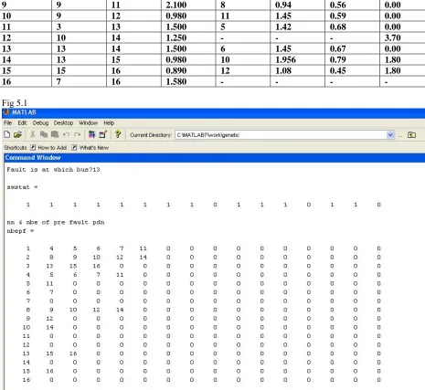
Step 2: Obtain the Connectivity of the pre-fault PDN using New Network Connectivity Method. Form the Matrix of nodes beyond a particular node ‘nbe’.
Step 3: Perform the Load Flow Analysis Using Forward Substitution Method.
Step 4: Compute the line flows and also the branch currents in various sections of the feeders.
Step 5: Check whether any fault is occurred? If there is any occurrence of fault, go to the next Step, otherwise go to Step 27.
Step 6: Check whether the fault is symmetrical or unsymmetrical. If the fault is symmetrical, form the Zbus of the distribution network using [16]. If the fault is unsymmetrical, form the positive, negative and zero sequence impedance matrices of the post fault PDN using [16].
Step 7: Set the generation count, Gen = 1.
Step 8: Obtain the Network Connectivity of the post fault PDN using the algorithm explained in Section 2 of this paper. Form the Matrix of nodes beyond a particular node ‘nbe’.
Step 9: Select the population size based on the number of branches in the EPDS. Choose the length of the chromosome as same as that of total number of buses in the PDN.
Step 10: Consider the loads in the order of their highest priority using preemptive method.
Step 11: Perform the load flow analysis using forward substitution method and then, calculate the post fault voltages of the PDN.
Step 12: Compute real and reactive power line flows, real and reactive power losses in the PDN. Step 13: Compute all the objectives of the objective function f1, f2, f3, f4, f5, f6 and f7.
Step 14: Compute the objective function ‘F’ for each Chromosome.
Step 15: Evaluate the fitness of the individual chromosomes in the population under consideration. Step 16: Rank the fitness function values in the ascending order.
Step 17: Perform selection of the individuals in the population. Step 18: Perform the crossover between the chromosomes. Step 19: Perform Mutation of individuals in the population.
Step 20: Form the new set of objective functions based on the new population.
Step 21: Check whether the constraints are met or whether the number generations reached maximum generation limit or not. If yes go to Step 24, otherwise go to next Step.
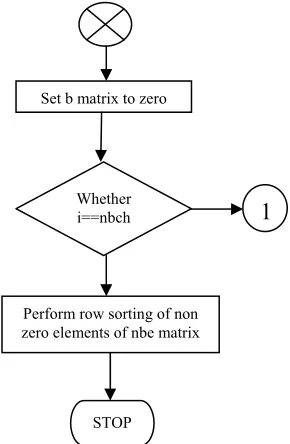
Set b matrix to zero
Whether
i==nbch
1
Perform row sorting of non zero elements of nbe matrix
Vol. 2(6), 2010, 1640-1650
Step 22: Convert the new objective function value to binary equivalent, and then perform the logical OR operation of this binary equivalent with to the old chromosomes.
Step 23: Update the generation count Gen = Gen + 1; and then go to Step 8.
Step 24: Perform the load flow analysis for the new reconfigured post fault PDN. Compute the line losses, power supplied from the substation and also calculate the real and reactive power line losses.
Step 25: Estimate operating time of the all the associated relays/breakers in the post fault PDN. Step 26: Compute the total restoration time.
Step 27: Print the results.
Step 28: If any further fault analysis is to be carried out for operational planning of EPDS go to Step 1, otherwise go to next Step.
Step 29: Stop.
S5.Results
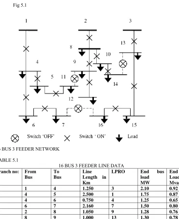
Fig 5.1
16 BUS 3 FEEDER NETWORK
TABLE 5.1
16 BUS 3 FEEDER LINE DATA
Branch no: From Bus
To Bus
Line
Length in Km
LPRO End bus load
MW
End bus Load
Mvar
Qsh in Mvar
1 1 4 1.250 3 2.10 0.92 0.00 2 4 5 2.500 1 1.75 0.87 1.10 3 4 6 0.750 4 1.25 0.65 1.20 4 6 7 2.160 7 1.50 0.80 0.00 5 2 8 1.050 9 1.28 0.76 0.00 6 8 9 1.000 13 1.30 0.78 1.20 7 8 10 0.790 2 1.65 0.78 0.00
9 9 11 2.100 8 0.94 0.56 0.00 10 9 12 0.980 11 1.45 0.59 0.00 11 3 13 1.500 5 1.42 0.68 0.00 12 10 14 1.250 - - - 3.70 13 13 14 1.500 6 1.45 0.67 0.00 14 13 15 0.980 10 1.956 0.79 1.80 15 15 16 0.890 12 1.08 0.45 1.80
16 7 16 1.580 - - - -
Vol. 2(6), 2010, 1640-1650
Result of reconfigured network
Fig 5.2
6. Discussion
Here it has been assumed that a line to ground fault takes place at the bus 13 with a fault impedance of 0.l p.u. Due to the occurrence of fault, the relay/breaker connected between buses 3 and 13 is operated and hence bus 13 gets isolated from the power supply. Due to operation of the breaker the power supply also gets disconnected to the loads which are connected to the buses 15 and 16. Hence the loads connected to the buses 15 and 16 are in dark state. In order to restore the power supply to the loads which are connected to the buses 15 and 16, the distribution network has to be reconfigured. The search of optimal configuration of PDN has been done using GA. For the 16-Bus EPDS, the GA parameters are selected as follows:
Length of the Chromosome = 16 Population size = 16
Probability of crossover = 0.7
Probability of mutation = 0.7/16 = 0.04375
The Optimal Configuration of post-fault PDN has been obtained using the GA.The status switches of the in optimal configuration of the PDN are given as follows:
SWSTAT=[1 1 1 1 1 1 1 0 1 1 0 1 0 0 1]
References
[1] Mohan MR, Manjunath K. A new hybrid multi-objective quick service restoration technique for electric power distribution systems. Science Direct issue Electrical power and energy systems 29 (2007) 51-64
[2] Mohan MR, Manjunath K. An improved technique for the estimation of service restoration time in power distribution systems. Int J Power Energy Syst,PowerCon Special Issue 2004;64-70.
[4] Manjunath K, Mohan MR. A new genetic algorithm based loss minimization and service restoration technique for distribution feeder reconfiguration. In: Proc IEEE national conference ACE – 2002, PW-41, Kolkata. p. 458–61
[5] Young-Hyun Moon, Se-Ho Kim, Bok-Nam Ha, Jung-Ho Lee. Fast and Reliable Distribution Load Flow Algorithm Based on the Ybus Formulation.
[6] S.Civanlar, J.J. Grainger, H. Yin, S.S.H. Lee. Distribution feeder reconfiguration for loss reduction. IEEE Trans on Power Delivery, vol 3. No.3,july 1988 p.1217-23
[7] Gareth P. Harrison, Antonio Piccolo, Pierluigi Siano, A. Robin Wallace. Hybrid GA and OPF evaluation of network capacity for distribution generation connections. Electrical Power Systems Research 78(2008) p. 392-98
[8] B.Venkatesh, Rakesh Ranjan .Optimal Radial Distribution System Reconfiguration using Fuzzy Adaption of Evolutionary Programing. Electrical Power & Energy Systems 25 (2003) p. 775-80
[9] H.A Taha, Operations research: An introduction(New York; Prentice Hall,2002).
[10] I.J Nagarath & D.P. Kothari, Power system engineering(New Delhi: TataMcgraw Hill, 1969)