COMPARISON OF ANN WITH RSM IN
PREDICTING SURFACE ROUGHNESS
WITH RESPECT TO PROCESS
PARAMETERS IN Nd: YAG LASER
DRILLING
ARINDAM MAJUMDERMechanical Engineering Department, National Institute of Technology, Agartala, Tripura- 799055, India
Abstract:
Micro machining is a ready solution towards the miniaturization of component and devices. The process parameters of low power pulse Nd:YAG laser machining such as pulse rate, pulse width, speed play a major role in deciding the surface quality. Two methods, response surface methodology (RSM) and artificial neural network (ANN) were used to predict the surface roughness of Nd:YAG laser drilled mild steel specimens. The experiments were conducted based on the three factors, three levels and central composite face centered design with full replication technique and mathematical model was developed. Also a comparison has been done with between the result obtained through response surface methodology (RSM) and artificial neural network (ANN).
Keywords
: Nd:YAG laser drilled; response surface methodology (RSM); artificial neural network (ANN).
1. INTRODUCTION
Laser beam machining is a method of cutting metal or refractory materials by localized melting and subsequently vaporizing the unintended material from the parent material with an intense beam of laser light from a laser source. The beam of the light is used to manufacture small-diameter holes that can be spaced along a layout line to cut materials. Applications of LBM are limited to cutting, drilling or welding thin metals and materials. Laser beam machining (LBM) is one of the most extensively used thermal energy based non-contact type advance machining process which can be applied for wide variety of materials. It is perfectly suitable for geometrically complex profile cutting and making miniature holes in sheet metal. Among various type of lasers used for machining in industries, CO2 and ND: YAG lasers are the most established lasing materials.
Laser in short bursts has a power output nearly 10 kw/cm2 of beam cross section. The sum total of radiation is 7
KW/cm2 on its surface. By focusing laser beam on a spot 1/100 of mm2 in size, the beam will be concentrated in
short flash to a power density of 10, 0000 KW/cm2. This is enough heat to melt and vaporize all high strength
engineering materials and permits the fusion and welding of refractory substances and metals.
is very important to select and control the process parameters for obtaining the optimum surface roughness. Various prediction methods can be applied to define the desired output variables through developing mathematical models to specify the relationship between the input parameters and output variables. The response surface methodology (RSM) is helpful in developing a suitable approximation for the true functional relationship between the independent variables and the response variable that may characterize the nature of the machining. It has been proved by several researchers [3-7] that efficient use of statistical design of experimental techniques, allows development of an empirical methodology, to incorporate a scientific approach.
Recently, in the fields of materials joining, computer aided artificial neural network (ANN) modeling has gained increased importance. In the several previous investigations it has been found that artificial neural network (ANN) modeling is one of the best methods to find a relation between the predictor variables (independents, inputs) and predicted variables (dependents, outputs) exists, even when that relationship is very complex and not easy to articulate in the usual terms of “correlations” or “differences between groups” [8, 9].
In the present investigation a mathematical model, by using response surface methodology (RSM) and an artificial neural network (ANN) model [10] has been generated to predict the relationship between the process parameter of Nd: YAG laser drilling and the surface roughness of the specimens. Also a comparison has been done with between the result obtained through response surface methodology (RSM) and artificial neural network (ANN).
2. MATERIAL:
The materials used in this experiment are mild steels (Carbon: 0.1-0.25 %) having thickness 0.65 mm.
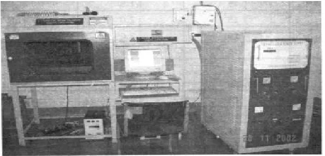
FIG. 1: ND: YAG LASER MACHINING SET UP
3. EXPERIMENTAL PROCEDURE
A CNC controlled SI Laser SLIP 200 Nd:YAG laser machine with three axis control is used for drilling (fig. 1). The machine basically consists of a laser resonator and beam delivery unit, power supply unit, cooling unit and CNC controller for X, Y and Z axis moment. The specification of the machine is given in the TABLE 1.
TABLE: 1
SPECIFICATIONS OF THE LASER SYSTEM
Model SLP-200 Average Power 200 W
Pulse Energy @ 20 ms 50 J Peak Power 7 KW Pulse with the range 0.3- 20 ms Pulse repetition rate 1-250 Hz
Work table size 450mm×600mm×150mm Power requirement 3 phase 440 V AC 20 Amps
The existing pulsed Nd:YAG laser system has been used to try out micro drilling for mild steel specimens. For this experiment pulse width, pulse repetition rate and the cutting speed are the key parameters identified to the control the cutting operations and hence are considered for investigations
The surface roughness measurements of the workpieces are done by using Taylor Hobson Surtronic machine. The specifications of surface measurement instruments are as shown in the TABLA 2.
TABLE: 2
SPECIFICATIONS OF THE SURFACE ROUGHNESS MEASURING INSTRUMENTS
Measurement range:
Minimum Value 0.01 µm Maximum Value ± 150 µm
Accuracy 2 % value + 1 min value
For measuring the surface roughness of the samples of thickness of one 0.65 mm mounting fixture has been developed which consists of five slots for holding the samples cut by laser process.
The surface morphology of the laser drilled holes as well as the spatter formation, as suited using a scanning electron microscope. After completion of geometrical measurements, the laser drilled samples are sectioned using a wire cut EDM, mounted on the fixture and sequentially ground to the centre of the hole.
In this present investigation the chosen process parameters and their level are presented in the TABLE 3.
TABLE: 3
INFLUENCE OF PULSE REPETITION RATE, PULSE WIDTH AND SPEED ON THE SURFACE ROUGHNESS VALUES OF THE LASER DRILLED HOLE
SL. NO. Pulse rate , H (Hz)
Pulse width, W (ms)
Speed, T (mms-1)
Surface roughness, Ra (µ inches)
1 10 1.5 1 131
2 10 1.5 1 131
3 10 1.5 2 221.5
4 10 1.5 3 409
5 10 2 1 150.45
6 10 3.9 1 236.67
7 15 1.5 1 110.4
8 15 1.5 2 157
9 15 1.5 3 156.33
10 15 1.5 3 156.33
11 15 2 1 114.83
12 15 2 1 114.83
13 15 2 2 187.17
14 15 2 2 187.17
15 15 2 3 185.33
16 15 3.9 1 117.33
17 15 3.9 1 117.33
18 15 3.9 2 146.33
19 20 1.5 1 102.5
20 20 1.5 2 122.17
21 20 1.5 2 122.17
22 20 1.5 3 127.33
23 20 1.5 3 127.33
24 20 2 1 101.43
25 20 3.9 1 110.23
Sample Length
Longer Wave 0.03 inch Shorter Wave 2.5 µm
4. DEVELOPMENT OF MATHEMETICAL MODEL 4.1. Response surface methodology
Response surface methodology (RSM) is a collection of mathematical and statistical technique useful for analyzing problems in which several independent variables influence a dependent variable or response and the goal is to optimize the response [11]. In many experimental conditions, it is possible to represent independent factors in quantitative form as given in Eq. (1). Then these factors can be thought of as having a functional relationship or response as follows:
……… (1)
Between the response Y and x1, x2, ………….., xk of k quantitative factors, the function Ø is called response
surface or response function. The residual er measures the experimental errors. For a given set of independent
variables, a characteristic surface is responded. When the mathematical form of Ø is not known, it can be approximate satisfactorily within the experimental region by polynomial. In the present investigation, RSM has been applied for developing the mathematical model in the form of multiple regression equations for the quality characteristic of the Nd: YAG Laser drilled mild steel specimens. In applying the response surface methodology, the independent variable was viewed as a surface to which a mathematical model is fitted. The second order polynomial (regression) equation used to represent the response surface Y is given by [12]
………… (2)
and for three factors, the selected polynomial could be expressed as
R
b
b H
b W
b T
b
H
b
W
b
T
b
HW
b
WT
b
TH
…..………… (3)
In order to estimate the regression coefficients, a number of experimental design techniques are available. In this work, central composite face centered design (Table 4) was used which fits the second order respons surfaces very accurately. Central composite face centered (CCF) design matrix with the star points being at the center of each face of factorial space was used, so α= ±1. This variety requires three levels of each factor. CCF designs provide relatively high quality predictions over the entire design space and do not require using points outside the original factor range. The upper limit of a factor was coded as +1, and the lower limit was coded as –1. The chosen levels of the selected process parameters with their units and notations are presented in TABLE 4.All the coefficients were obtained applying central composite face centered design using the Design Expert statistical software package. After determining the significant coefficients (at 95% confidence level), the final model was developed using only these coefficients and the final mathematical model to estimate tensile strength is given:
47.20136
35.27698
206.86417
316.61443
4.54072
11.49471
19.10174
1.72279
18.68102
14.72433
……. (4)TABLE: 4
IMPORTANT ND: YAG PROCESS PARAMETERS AND THEIR LEVELS
Parameter Level
(-1) (0) (1)
Pulse rate , H (Hz) 10 15 20
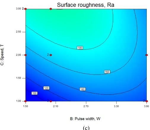
Pulse width, W (ms) 1.5 2 3.9 Speed, T (mms-1) 1 2 3 Fig. 2 and Fig. 3 present three dimensional response surface plots and contour plot for the response surface
(a)
FIG.2: RESPONSE PLOTS OF PROCESS PARAMETERS ON SURFACE ROUGHNESS
(c)
(a)
FIG.3:CONTOUR PLOTS OF PROCESS PARAMETERS ON SURFACE ROUGHNESS
4.2. Checking Adequacy of The Model
The adequacy of the developed model was tested using the analysis of variance (ANOVA) technique and the results of second order response surface model fitting in the form of analysis of variance (ANOVA) are given in Table 5. The determination coefficient (R2) indicates the goodness of fit for the model.In this case, the value of the
determination coefficient (R2=0.8929) indicates that only less than 10% of the total variations are not explained by
the model. The value of adjusted determination coefficient (adjusted R2=0.8287) is also high, which indicates a high
significance of the model.
TABLE: 5
ANOVA FOR RESPONSE SURFACE QUADRATIC MODEL
Source Sum of Squares
df Mean Square
F Value p-value Prob > F
Model 88566.68 9 9840.742 13.90217 < 0.0001 significant
A-A 44418.64 1 44418.64 62.75091 < 0.0001
B-B 0.510722 1 0.510722 0.000722 0.9789
C-C 3227.522 1 3227.522 4.559572 0.0496
AB 3842.2 1 3842.2 5.427936 0.0342
AC 21654.37 1 21654.37 30.59147 < 0.0001
BC 1286.579 1 1286.579 1.81757 0.1976
A2 8805.195 1 8805.195 12.43924 0.0031
B2 1244.191 1 1244.191 1.757689 0.2048
C2 845.0335 1 845.0335 1.193792 0.2918
Residual 10617.85 15 707.8565 Lack of Fit 10617.85 8 1327.231
Pure Error 0 7 0 Cor Total 99184.52 24 R2 = 0.8929 Adj-R2= 0.8287
Pred-R2= 0.5638 Adeq Precisor= 16.688
The normal probability plot of the residuals for surface roughness shown in Fig.4 reveals that the residuals are falling on the straight line, which means the errors are distributed normally [13]. All the above consideration
indicates an excellent adequacy of the regression model. Each observed value is compared with the predicted value calculated from the model in Fig.5.
FIG.4:NORMAL PROBABILITY PLOT OF RESIDUALS FOR TENSILE STRENGTH
FIG.5:PLOT OF ACTUAL VS PREDICTED RESPONSE OF TENSILE STRENGTH
5. ARTIFICIAL NEURAL NETWORK (ANN)
hidden layer neurons and 1 to the output. The topology architecture of feed-forward three-layered back propagation neural network is illustrated in Fig.6. MATLAB 7.1 was used for training, testing and validation of the network model for surface roughness prediction. The neural network described in this work, after successful training, was used to predict the surface roughness of Nd: YAG laser drilled mild steel specimens within the trained range. Statistical methods were used to compare the results produced by the network. Errors occurring at the learning and testing stages are called the root-mean square (RMS), absolute fraction of variance (R2), and mean error percentage
values. These are defined as follows, respectively:
∑
/ ∑
……… (5)Where Yp is the predicted (using the above model), Ye is the experimental value, Ya is the average of experimental
values.
FIG.6:ANN ARCHITECTURE USED
5.1. Result from The Neural Network Analysis
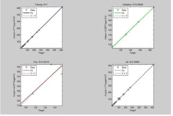
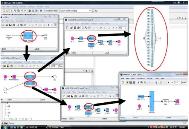
The results obtained from the analysis were extremely satisfactory and a very high value of regression was obtained. The following performance curve was obtained on training, testing and validation of the data using MATLAB 7.1. The performance of the network was satisfying with the MSE of 3.938e-27 as shown in Fig. 7. The regression plot of output vs. target was obtained with 20 hidden nodes and regression value of 0.9987 was reached (Fig.8). This shows the validation of the model. The SIMULINK MODEL thus obtained is as shown in
FIG. 7: PERFORMANCE CURVE OBTAINED FOR THE ARTIFICIAL NEURAL NETWORK
FIG. 9: SIMULINK MODEL OF NEURAL NETWORK ANALYSIS
6. COMPARISON OF ANN AND RS MODELS
The trend in the modeling using RSM has a low order non-linear behavior with a regular experimental domain and relatively small factors region, due to its limitation in building a model to fit the data over an irregular experimental region. Moreover, the main advantage of RSM is its ability to exhibit the factor contributions from the coefficients in the regression model. This ability is powerful in identifying the insignificant main factors and interaction factors or insignificant quadratic terms in the model and thereby can reduce the complexity of the problem. On the other hand, this technique requires good definition of ranges for each factor to ensure that the response(s) under consideration changes in a regular manner within this range. It is noted that ANNs perform better than the other techniques, especially RSM when highly non-linear behavior is the case. Also, this technique can build an efficient model using a small number of experiments; however, the technique accuracy would be better when a larger number of experiments are used to develop a model. On the other hand, the ANN model itself provides little information about the design factors and their contribution to the response if further analysis has not been done. Generation of ANN model requires a large number of iterative calculations whereas it is only a single step calculation for a response surface model. Depending on the nonlinearity of the problem and the number of parameters, an ANN model may require a high computational cost to create. Although computationally much more costly than a response model, ANN model leads to comparatively accurate surface roughness predictions as shown in Table 6.
TABLE: 6
COMPARISON BETWEEN RSM AND ANN
Model summary and prediction errors
Response surface methodology(RSM)
Artificial neural network(ANN) Root mean square
(RMS)
20.3 3.102
R2 0.8929 0.99887
Computational time Short Short Understanding Easy Moderate
FIG.10COMPARISON OF OBSERVATION ORDER WITH RESIDUALS
CONCLUSIONS
This paper has described the use of design of experiments (DOE) for conducting experiments. Two models were developed for predicting surface roughness of Nd: YAG Laser drilled mild steel specimens using response surface methodology (RSM) and artificial neural network (ANN).The predictive ANN model is found to be capable of better predictions of tensile strength within the range that they had been trained. The results of the ANN model indicate it is much more robust and accurate in estimating the values of tensile strength when compared with the response surface model.
ACKNOWLEDGEMENTS
The author gratefully acknowledges the help of the Department of Mechanical Engineering, Machine Shop of National Institute of Technology, Agartala-799055, for their kind co-operation and help in this project.
REFERENCES
[1] Koechner, Waiter. (1988); - ‘Solid-State Laser Engineering’- 2nd edition, Springer-Verlag. ISBN 3-540-18747-2.
[2] Geusic. J. E., Marcos. H. M. and Van Uitert. L, G. (1964) ;-‘ Laser Oscillations in Nd- doped Yttrium Aluminum, Yttrium Gallium and
Gadolinium Garnets’- Applied Physics Letters, Vol. 10, pp- 182-184.
[3] GRUM J, SLABE J M. (2004). The use of factorial design and response surface methodology for fast determination of optimal heat
treatment conditions of different Ni-Co-Mo surfaced layers [J]. Journal of Materials Processing Technology, 155, pp- 2026-2032.
[4] Box, G.E.P., Hunter, W.G., and Hunter, J.S., (1978), Statistics for Experimenters, John Wiley & Sons, NY.
[5] Montgomery, D. C. (2000), Design and Analysis of Experiments, Wiley, New York. 5th Edition.
[6] D.C. Montgomery and G.C. Runger. (1994), Applied Statistics and Probability for Engineers, John Wiley and Sons, Inc, New York.
[7] J.A. Cornell, A.I. Khuri. (1987), Response surfaces: Designs and Analysis, Marcel Dekker, New York.
[8] Patterson, D. (1996). Artificial Neural Networks. Singapore: Prentice Hall. Good wide-ranging coverage of topics, although less detailed
than some other books.
[9] Ripley, B.D. (1996). Pattern Recognition and Neural Networks. Cambridge University Press. A very good advanced discussion of neural
networks, firmly putting them in the wider context of statistical modeling.
[10] DUTTA P, PRATIHAR D K. (2007) Modeling of TIG welding process using conventional regression analysis and neural network-based
approaches [J]. Journal of Materials Processing Technology, 184: 56-68.
[11] COCHRAN, COX G M. (1962) Experimental design [M]. New Delhi: Asia Publishing House.
[12] BALASUBRAMANIAN M, JAYABALAN V, BALASUBRAMANIAN V. (2008) A mathematical model to predict impact toughness of
pulsed current gas tungsten arc welded titanium alloy [J]. Journal of Advanced Manufacturing Technology, 35(9/10): 852-858.
[13] KUMAR S, KUMAR P, SHAN H S. (2007) Effect of evaporative casting process parameters on the surface roughness of Al-7%Si alloy
castings [J]. Material Processing Technology, 182: 615-623.
[14] ZHANG Z, FRIEDRICH K. (2003) Artificial neural networks applied to polymer composites: A review [J]. Composites Science and
Technology, 63: 2029-2044.
[15] ARCAKHOGLU E, CAVUSOGLU A, ERISEN A. (2004) Thermodynamic analyses of refrigerant mixtures using artificial neural networks
[J]. Applied Energy, 78: 219-230.