Visual Perception For Robotic Spatial Understanding

(1)

University of Pennsylvania

ScholarlyCommons

Publicly Accessible Penn Dissertations

2019

Visual Perception For Robotic Spatial

Understanding

Jason Lawrence Owens

University of Pennsylvania, jlowens@gmail.com

Follow this and additional works at:https://repository.upenn.edu/edissertations

Part of theArtificial Intelligence and Robotics Commons, and theRobotics Commons

This paper is posted at ScholarlyCommons.https://repository.upenn.edu/edissertations/3242

For more information, please contactrepository@pobox.upenn.edu.

Recommended Citation

(2)

Visual Perception For Robotic Spatial Understanding

Abstract

Humans understand the world through vision without much effort. We perceive the structure, objects, and people in the environment and pay little direct attention to most of it, until it becomes useful. Intelligent systems, especially mobile robots, have no such biologically engineered vision mechanism to take for granted. In contrast, we must devise algorithmic methods of taking raw sensor data and converting it to something useful very quickly. Vision is such a necessary part of building a robot or any intelligent system that is meant to interact with the world that it is somewhat surprising we don't have off-the-shelf libraries for this capability.

Why is this? The simple answer is that the problem is extremely difficult. There has been progress, but the current state of the art is impressive and depressing at the same time. We now have neural networks that can recognize many objects in 2D images, in some cases performing better than a human. Some algorithms can also provide bounding boxes or pixel-level masks to localize the object. We have visual odometry and mapping algorithms that can build reasonably detailed maps over long distances with the right hardware and conditions. On the other hand, we have robots with many sensors and no efficient way to compute their relative extrinsic poses for integrating the data in a single frame. The same networks that produce good object segmentations and labels in a controlled benchmark still miss obvious objects in the real world and have no mechanism for learning on the fly while the robot is exploring. Finally, while we can detect pose for very specific objects, we don't yet have a mechanism that detects pose that generalizes well over categories or that can describe new objects efficiently.

We contribute algorithms in four of the areas mentioned above. First, we describe a practical and effective system for calibrating many sensors on a robot with up to 3 different modalities. Second, we present our approach to visual odometry and mapping that exploits the unique capabilities of RGB-D sensors to efficiently build detailed representations of an environment. Third, we describe a 3-D over-segmentation technique that utilizes the models and ego-motion output in the previous step to generate temporally consistent segmentations with camera motion. Finally, we develop a synthesized dataset of chair objects with part labels and investigate the influence of parts on RGB-D based object pose recognition using a novel network architecture we call PartNet.

Degree Type

Dissertation

Degree Name

Doctor of Philosophy (PhD)

Graduate Group

Computer and Information Science

First Advisor

(3)

Keywords

calibration, computer vision, mapping, object parts, object recognition, visual odometry

Subject Categories

(4)

VISUAL PERCEPTION FOR ROBOTIC SPATIAL UNDERSTANDING

Jason Owens

A DISSERTATION

in

Computer and Information Science

Presented to the Faculties of the University of Pennsylvania

in

Partial Fulfillment of the Requirements for the

Degree of Doctor of Philosophy

2019

Supervisor of Dissertation:

Kostas Daniilidis, Ruth Yalom Stone Professor Department of Computer and Information Science

Graduate Group Chairperson:

Rajeev Alur, Zisman Family Professor

Department of Computer and Information Science

Dissertation Committee:

Camillo J. Taylor, Professor, Department of Computer and Information Science

Jianbo Shi, Professor, Department of Computer and Information Science

Jean Gallier, Professor, Department of Computer and Information Science

(5)

(6)

(7)

Acknowledgments

The completion of my PhD would not have been possible without the support,

un-derstanding, and patience of my amazing wife Nettie and my children J, M and E. It

is to them that I owe my deepest gratitude. So far, my children have endured most

of their living memory with Daddy “going to school,” and I am happy to finally begin

the next chapter of our lives together!

I am very thankful for the support of my parents and my in-laws. My parents

worked hard to give me the best opportunities and encourage me at every step.

Throughout my entire trip at Penn, my in-laws have been there for me and my wife

and kids, and have helped to provide space, time, food, and adult beverages when

needed most. I am grateful and humbled to have such a caring family.

Many of my colleagues at ARL have been with me the entire time; encouraging,

listening, commiserating, and otherwise tolerating my ups and downs through this

degree. I especially thank Mr. Phil Osteen for being the most patient, thoughtful

and supportive collaborator and friend. Not only do most of my papers have his

name on them, but he often provided the steady head that helped us get through

some of the most challenging deadlines, no matter what the cost. I also thank my

other colleagues and friends that have been there to listen to my stories and provide

support, including (but not necessarily limited to) Dr. MaryAnne Fields, Dr. Chad

Kessens, Mr. Jason Pusey, Mr. Ralph Brewer, and Mr. Gary Haas.

I would like to thank Dr. Drew Wilkerson for strongly encouraging me to use the

opportunities through the DOD and the Army Research Laboratory to pursue this

education and degree. I must also thank Dr. Jon Bornstein for continuing to support

(8)

Geoff Slipher continued the tradition, and helped me get through the final hurdles; I

am grateful for his consideration and understanding during this final year. Finally, I

must thank ARL as an organization for the opportunity and privilege of attending a

school such as the University of Pennsylvania; this has truly been a once in a lifetime

experience.

I thank Dr. Richard Garcia for his friendship, support, and our drives to and from

Philadelphia to attend Prof. Taskar’s (Requiescat in pace) machine learning class.

I thank LTC Christopher Korpela, PhD. for crashing on my couch in Philly during

hisdegree, and otherwise being a good friend and role model for getting $#!+ done.

What would time at the GRASP lab be but for my fellow students grinding

through their degrees? I would like to thank Christine Allen-Blanchette for our many

office discussions ranging over a wide variety of topics; always interesting, always

stim-ulating, usually too short :-) I am grateful for my discussions with Matthieu Lecce; he

helped me see I’m not the only one. I am very grateful for Kostas’ Daniilidis Group

discussions; the brainpower in that group is phenomenal. So many great explanations

and just general geeking out.

I would like to thank the professors at Penn I’ve had the privilege to learn from

and interact with, both in my capacity as a student and ARL researcher. I

specif-ically thank Prof. C.J. Taylor for chairing my dissertation committee and always

asking the hardest questions. I’m grateful to Prof. Jean Gallier for participating in

my committee, and for the many enjoyable and amusing discussions across the

hall-way. I thank Prof. Jianbo Shi for offering his time for both technical and personal

discussions, including several tips to help my kids do their piano practice. While not

a Penn professor, I also must thank Prof. Nick Roy from MIT for being a part of my

committee, and for helping me recognize the work I’ve done.

Last, but most definitely not least, I must thank my adviser and friend, Prof.

Kostas Daniilidis, who patiently supported me, argued for me, and gently guided me

through my stubborness for my many years in this program. He did what he could

to pull me along, but I was often too hard-headed to comply; while I’m sure there is

(9)

to work together no matter what our respective circumstances might be. Thank you,

Kostas!

For those whose names I left out (and I know there are many), I most sincerely

thank you. Keep working hard and always do the right thing. But never forget to

(10)

ABSTRACT

Jason Owens

Kostas Daniilidis

Humans understand the world through vision without much effort. We perceive the structure, objects, and people in the environment and pay little direct attention to most of it, until it becomes useful. Intelligent systems, especially mobile robots, have no such biologically engineered vision mechanism to take for granted. In contrast, we must devise algorithmic methods of taking raw sensor data and converting it to something useful very quickly. Vision is such a necessary part of building a robot or any intelligent system that is meant to interact with the world that it is somewhat surprising we don’t have off-the-shelf libraries for this capability.

Why is this? The simple answer is that the problem is extremely difficult. There has been progress, but the current state of the art is impressive and depressing at the same time. We now have neural networks that can recognize many objects in 2D images, in some cases performing better than a human. Some algorithms can also provide bounding boxes or pixel-level masks to localize the object. We have visual odometry and mapping algorithms that can build reasonably detailed maps over long distances with the right hardware and conditions. On the other hand, we have robots with many sensors and no efficient way to compute their relative extrinsic poses for integrating the data in a single frame. The same networks that produce good object segmentations and labels in a controlled benchmark still miss obvious objects in the real world and have no mechanism for learning on the fly while the robot is exploring. Finally, while we can detect pose for very specific objects, we don’t yet have a mechanism that detects pose that generalizes well over categories or that can describe new objects efficiently.

(11)

List of Tables

2.1 An overview of selected ego-motion algorithms reviewed in this section

and their attributes. . . 24

4.1 Examples of military work tasks for robots. . . 62

5.1 Average Frame-to-Frame Rotational Error (radians) . . . 123

5.2 Average Runtime (seconds) . . . 123

8.1 Training parameters for our experiments. . . 182

8.2 The mAP for PartNet at two common IOU thresholds. This score only considers regions the network detects as compared to ground truth. . 185

(14)

List of Figures

1.1 A near-ideal segmentation of a street scene. . . 7

2.1 Scaramuzza et al compute an extrinsic calibration between a 3D laser range finder and a camera . . . 12

2.2 Le and Ng’s multi-sensor graph calibration . . . 13

2.3 Maddern et al. calibrate 2D and 3D laser range finders to a robot frame 14 2.4 libviso2visual odometry system. . . 16

2.5 Example DVO image warping. . . 17

2.6 Loop closing example. . . 20

2.7 ORB-SLAM feature and map density. . . 21

2.8 Levinshtein et al. compare their TurboPixel over-segmentation algo-rithm to others . . . 27

2.9 Hu et al. apply a fixed volumetric discretization to generate an efficient over-segmentation . . . 28

2.10 Finman et al. apply a modified version of Felzenszwalb and Hutten-locher efficient graph based segmentation to slices of a TSDF model . 29 2.11 PoseCNN from Xiang et al. . . 31

2.12 PoseAgent from Krull et al. is an RL agent that selects pose hypotheses for refinement . . . 35

2.13 Gupta et al. match CAD models to segmented instances . . . 38

2.14 Grabner et al. estimate 3D bounding boxes and fit CAD models to RGB images . . . 40

2.15 Fischler and Elschlager construct templates based on explicit and se-mantic parts. . . 42

2.16 Felzenszwalb and Huttenlocher extend the pictorial structures frame-work of Fischler and Elschlager . . . 43

2.17 Example part primitives from Tulsiani et al. . . 45

3.1 A Hokuyo UTM-30 scanning laser rangefinder . . . 48

3.2 A simple pinhole camera model . . . 51

4.1 An example camera-colored 3D LRF frame from the calibration data collection. . . 64

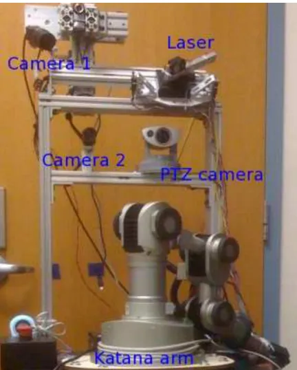
4.2 The robot sensors we calibrate . . . 70

4.3 The structure of the 3D laser range finder . . . 81

(15)

4.5 Simulation results . . . 85

4.6 Example fused laser and camera data for the Husky sensors . . . 86

5.1 EGI and associated histogram . . . 115

5.2 Feature matching comparison . . . 118

5.3 In-house data set testing results . . . 119

5.4 Sparse features sets induce VO failure . . . 120

5.5 10Hz room benchmark data set comparison . . . 121

5.6 360°10Hz data set comparison . . . 122

5.7 Downsampled data set results . . . 124

5.8 Reconstructed point clouds over the investigated algorithms . . . 124

6.1 Our SLAM system diagram . . . 134

6.2 An example model of a captured living room . . . 139

6.3 Model of a section of two offices and a hallway . . . 140

6.4 Another office model capture before the loop closure. . . 141

6.5 A captured model of a playroom . . . 142

6.6 Multiple views of a captured object . . . 142

7.1 The tree structure for a simple octree with three layers . . . 151

7.2 Purely incremental segmentation over multiple frames . . . 154

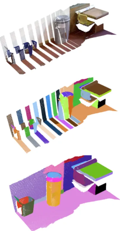
7.3 Comparison of segment changes, with and without boundary heuristic 157 7.4 RGB and depth images from the three scenes analyzed. . . 159

7.5 Runtimes and segment sizes for three segmentation algorithms on each dataset . . . 160

8.1 The PartNet architecture . . . 168

8.2 The segmentation network layers, listed left to right. . . 171

8.3 The translation branch layers of the pose network. . . 171

8.4 The rotation branch layers of the pose network. . . 172

8.5 Examples of part masks generated for the pose network . . . 173

8.6 The rotation representation hierarchy. . . 174

8.7 Exemplar SceneNet RGB-D frames . . . 179

8.8 Example chair renderings from our dataset. . . 180

8.9 Data images contained for each frame in the dataset . . . 181

8.10 Good and bad examples of part detection . . . 184

8.11 Orientation accuracy plotted against an angular threshold . . . 188

8.12 Translation accuracy plotted against a distance (in meters) threshold. 189 8.13 Rotation and translation broken down by input modality . . . 190

9.1 Example cuboid ground truth . . . 193

(16)

Chapter 1 Introduction

The story I tell here extends all the way back to my childhood. Robots and artificial

intelligence fascinated me. I had already been exposed to computers (an Apple IIc

and an Apple Macintosh 512K), and wondered how they worked. When I learned of

the concept of programming, the ability to make a computer do what you told it to

do, I knew I wanted to do it. Some years later, I saw some robots in a magazine—they

were Rodney Brooks’ and his students’ creations—and on a particularly nice day in

SoCal I wondered how it would be possible to make an engineered machine behave

intelligently. Of course, I really had no idea of the complexity and state-of-the-art at

the time, but it looked like Brooks had done something amazing1_{. The question has}

remained fixed in my mind since that particular sunny day in front of my parents’

house.

When I first started doing research related to robots, I was, therefore, particularly

interested in how one might get them to have intelligent behavior. What that really

meant was unclear, but it involved some combination of “moving around without

run-ning into things” and actually “accomplishing useful goals for humans and Soldiers.”

My initial conception developed into an interest in the topic of autonomous mental

development: i.e., the capability of a robot to learn how to function for one or more

tasks through interaction with the environment and without explicit programming

1_{I do believe Brooks (and his students) did accomplish something amazing, but it wasn’t exactly}

(17)

for any specific task. I wanted to (ultimately) develop a general “robot brain2_.”

As I began to investigate this line of research, I became frustrated with the state of

the art in robot perception and, for lack of a better word, a robot’s understanding

of the world. My concept of a robotic brain (at the time) hinged on the idea that the

world would be mostly observable and symbolic. This belief showed my utter naivet´e

at the time. The more I studied the literature, the more I came to understand that

getting an embodied robot to function the way I envisioned would require some

signif-icant improvement to how it could use vision (as well as other modalities) to interpret

the environment in a useable way. Again, I use another imprecise notion: “usability.”

I knew of the symbol grounding problem, and this was the exact embodiment of it.

To really be able to become intelligent, the things and stuff in the environment must

effectively become symbols that can be manipulated by an algorithm, and the symbols

must not stand alone (to borrow Harnad’s nomenclature [80], they should be related

to both iconic and categorical representations that themselves can be manipulated).

I assumed this algorithm would be complex, and the symbols would also be complex,

but I had no clue how to get from pixels or point clouds to symbols. Perhaps needless

to say, the goal of developing any version of a robot brain during my studies was

postponed, as it became apparent that we (as researchers, and as a field) had more

pressing problems on our hands.

Why is perception so important for robotics? First, I want to be precise about my

use of the term “robotics.” Robotics is a giant field, and covers many areas from what

I would call unintelligent automation through human-like embodied intelligent agents.

Throughout this document, I will use the terms ’robot’, ’agent’, and ’embodied

in-telligent agent’ interchangeably, but in all cases I am referring to the latter unless

explicitly stated. So, why is perception so important to embodied intelligent agents?

They need the ability to intelligently see and understand the environment in order to

participate effectively in the kinds of activities most useful to humans3. This desired

ability is usually called perception, and is in contrast to some other vision tasks that

2_{Yes, I have very ambitious and often unrealistic goals. It is a problem I’m trying to work on.} 3_{Especially the dirty, dangerous and/or defensive kind, but also the assistive, supportive and/or}

(18)

may not strive to enable the same level of intelligence. I also happen to believe that

a robot with sufficient perception capabilities is a prerequisite to anintelligent robot,

and that intelligence is required to have effective perception. They really go hand in

hand. While it is not the case that perception is the only thing holding us back, it

is an integral part of even the simplest system, and we must do everything we can to

enable this capability.

What do I mean by perception? As I mentioned already, a robot capable of

perception must “see and understand the environment.” This is a very compact way

to express a lot of ideas, so let’s unpack it. Seeing is the ability to separate, pick

out, and represent in some way or another, the important things in the environment.

Understanding is harder to define, but we interpret it as the ability to transform what

is seen into a meaningful and useful representation of the world. By “meaningful”,

we demand that the robot does more than determine a simple 1-1 mapping between

sensed data (e.g., pixels) and labels; instead, it implies the association of related

information such as experiences, similarities, differences and affordances as well as

a deeper recognition of structure (hierarchical, spatial, temporal) and the ability

to reason about what is sensed. All of this is necessary to make inferences about

the nature and purpose of the environment and the objects in it on a level similar

to a human. By “useful representation” we imply that there is more to the set of

pixels or points orn-dimensional vectors that are output by an algorithm. Certainly,

these elements may be part of the output, or even an integral component in the

representation itself, but they must be part of a larger whole that can be operated on

at multiple symbolic levels. Finally, the environment is everything around the robot,

including everything that can change over time and space.

To go beyond data transformation and interpret information in relation to past

experience and knowledge implies the need for reasoning capabilities typically

con-sidered outside the realm of computer vision (thus, my assertion that intelligence and

perception are tightly related). However, I believe the following high-level capabilities

are necessary for the task:

(19)

as the structure of the environment;

2. separating things from stuff [85];

3. learning object instances and categories, as well as perceiving the context

in-duced by the spatial relationships and configurations of the objects;

4. generalizing perceptual capability from previous experience.

These are not new ideas. However, they do provide the goals that motivate the

development of algorithms we can use to compose behaviors to achieve this

function-ality.

Most of the approaches in this dissertation involve an abstraction that raises the

level of semantic meaning of data, which corresponds well with the long-term goal

of pursuing intelligent perception. For example, the multi-sensor graph calibration

utilizes geometric representation and relationships between the sensed calibration

object from multiple sensors in order to relate the data and perform the optimization.

The primary goal of ego-motion estimation and the environment mapping was to use

surfels that contain more information than just points in order to aid the alignment

and mapping process. In temporal segmentation, we take point clouds and turn them

into segments using similarities in their spatial structure so that you could work with

larger logical chunks of the cloud instead of individual points or surfels within the

cloud. Finally, we tackle parts of objects. Here, it apparently looks like we’re taking

a step down, and it is true in one sense; however, we are really interested in gaining

more information about objects by understanding their composition and recognizing

their pose.

1.1 Motion and the environment

To learn in the way I have described, I believe intelligent systems that are meant

to interact with humans and the real world must actually be embedded in the real

(20)

will not happen by just looking at static pictures4_{. There must be understanding of}

how the world changes through differing viewpoints, how objects move and can be

manipulated, and how the environment is structured by nature and humans (Grauman

speaks directly of these topics in her latest talks on “Embodied Visual Perception”

[75]). To address capability 1 above, sensors must be mounted on a mobile platform

and must capture the true dynamic nature of the environment. This is in contrast to

much of the work in simultaneous localization and mapping (SLAM) and environment

mapping that tends to ignore the dynamic nature of the world. It is a hard problem,

but all the more important on account of that. A dynamic world gives significant

cues for object segmentation, 3 dimensional structure, and deformable objects.

We encounter our first obstacle after mounting multiple sensors on a robot. To

process the data in a coherent manner, or more specifically, in the same coordinate

frame of reference (usually with one sensor or the robot platform serving as the

origin), we must knowwhere the sensors are with respect to one another. This seems

like it should be a trivial problem: we mounted them on the robot, therefore we

should know where they are! Unfortunately, it is not that simple; first, every sensor

is different and every mounting configuration is different; second, we do not always

know the sensor’s origin, even if we assume or know it is intrinsically calibrated5_{. To}

begin to collect data from a robot with multiple sensors, whether all of one type (e.g.,

all cameras) or of multiple modalities (e.g., a camera, a two-dimensional (2D) laser

scanner, and a three-dimensional (3D) sensor), we must find the extrinsic calibration

of the entire system: the relative pose of each sensor with respect to some origin.

Chapter 4 discusses one approach to this challenge, and presents the only system

we are aware of that solves the problem for a statically mounted set of sensors with

multiple modalities and with very few requirements.

Having a robot with calibrated sensors means we can collect the sensor data into

4_{I’m looking at you, ImageNet. While this challenge has done much to spur development in}

algorithms for large scale recognition, it’s applicability to intelligent embodied systems is limited by it’s lack of focus on actually understanding the visual world; instead it focuses on generating mappings between pixels and labels without any accessible, underlying model.

5_{Third, I only consider rigidly mounted sensors in this dissertation. We are}

(21)

a common coordinate frame. Now we encounter a second obstacle: it would be

difficult for our embodied system to move around and manipulate the world without

understanding how it is structured and how it operates, at least at the local level (i.e.,

the portions of the environment it can currently see with the sensors). While I strongly

believe much of this knowledge needs to be represented in a shared and consistent

fashion, I also believe that larger problems must be broken down into chunks; therefore

I separate the structure from the operation, and examine algorithms for ego-motion

estimation and detailed environment mapping. Chapter 5 discusses our approach for

using RGB-D cameras to capture accurate motion and Chapter 6 uses the

ego-motion estimates to build up maps of the environment. In these chapters, we will also

discuss how these components may be used for extending the capability of robots in

the future.

1.2 Things and stuff

Knowing the structure of the world is only one part of the challenge. Efficient map

representations and planning algorithms may allow a robot to navigate the world, but

how will it begin to learn about the objects in the world? There must be some way

to partition the world into separate objects (usually the things we are interested in)

and the other stuff that the world is made of (e.g., walls, floors, grass, sky).

Achiev-ing capability 2 above is the job of a segmentation and object proposal algorithm.

While humans respond well to Gestalt cues (such as symmetry, continuity, common

fate) [108] and some have made efforts to incorporate these cues into algorithms for

object segmentation [101], [111]–[114], we focus on the under-explored topic of

over-segmenting a scene in a temporally consistent way. An over-segmentation is often

used as a pre-processing step, and helps later algorithms by clustering primitive

per-ceptual data into larger chunks that are typically spatially, visually, and geometrically

coherent. While many over-segmentation algorithms operate in image space only, in

Chapter 7, we modify an existing algorithm that operates on 3D point clouds to

(22)

Figure 1.1 A near-ideal segmentation of a street scene.

estimation and frame integration algorithm. This builds on the work from the

pre-vious section, and would not be possible without a good estimation of the sensor

motion.

Segmenting a scene (or the environment), the particular partitioning of what is

seen into chunks (hopefully as close to an ideal segmentation as possible, see Fig. 1.1),

is a prerequisite to being able to discover and learn about objects. While there are

attempts to do this in concert with object recognition [26], [82], [174], we believe

the best approach is to separate the task of segmentation and object proposals from

recognition, and ultimately focus on an iterative interplay between the algorithms.

Without this, it is not clear how to dynamically extend a recognition system with

new information on the fly.

1.3 Objects

It is clear that a robot cannot do much useful work without being able to first detect,

identify, and describe objects, and second, manipulate those objects. Objects are

a fundamental aspect of the world. They are the things we want to manipulate or

observe as well as the stuff that surrounds us. An intelligent embodied system must

be able to see objects in such a way as to determine their location, identity (up to

some extent), and category as well as whether and how they can be manipulated (i.e.,

their affordances). If a robot did not possess such a capability, most things would

simply be implictly classified as an obstacle, or otherwise occupied space.

(23)

of a specific object (e.g., a box of one kind of cereal), or as an instance of category,

whether specific or general. The first kind of recognition is used extensively in robots,

to handle a small sampling of real-world objects in a very specific way, by both

representing appearance and geometry of the object in order to detect presence and

pose simultaneously. However, this means that if it recognizes one cereal box, then it

may not recognize another, even if they are very similar in many ways: size, geometry,

general appearance (e.g., a lot of bright colors). The second kind of recognition, on

the other hand, is, by definition, more general, and refers to the ability to recognize

that a box of any brand of cereal is, in fact, a box of cereal. In many cases, however,

categorical object recognition (the most common type) is unable to recognize specific

instances, or even determine that box A and box B are the same kind of cereal.

Interestingly, humans perform both of these tasks pretty well, and it may prove to be

hard for robots to interact seamlessly and efficiently with their biological collaborators

without a similar level of proficiency.

The question remains: how do we induce an algorithm to “recognize” anything?

Research to address this question has been going on for over 50 years and we have

developed specific algorithms for detection (“am I looking at an object of instanceior

categoryk?”), localization (“where is the object and what is its pose”), and recognition

(“find and identify all known objects”) [3]. Detection, localization and recognition all

rely on some form of matching input data to previously learned models. As part of

that input data, we have strong evidence that the human visual system does extract

low level features early in the visual process [137], [207]. One of the basic ideas behind

the use of features is to find regions of interest in order to use them as descriptions

in a model of the object or environment such that it is possible to match the input

data to previously learned models, hopefully without a linear search.

While deliberately leaving the definitions of “feature”, “match”, “description”, and

“concept” vague, imagine we want to create a database of known objects for use in a

robotic vision task. We would like to extract salient features that could be used to

recognize these objects in new environments, where they may be seen in a variety of

(24)

features to make the object detection and recognition task more effective? If we want

to detect local features, we must consider a neighborhood surrounding a point to

determine whether that point actually represents the location of a feature. How do

we select the size of the neighborhood?

To answer some of these questions and work to address our previously stated

ca-pability 3, we propose to investigate convolutional networks that perceive additional

information about objects in the form of parts and pose. Most objects are composed

of more than one part, and often the parts may be individually recognizable

compo-nents. If not individually recognizable, then the collection of parts may still provide

additional useful information about the structure and pose of the object. While this

approach may not directly address the instance recognition task mentioned above, if

successful it could represent a significant improvement in pose estimation capability

for general object categories. We describe our initial approach and results in Chapter

8.

1.4 Generalization

Generalization is, in some ways, the holy grail of artificial intelligence, and therefore

most of its sub-fields, like robotic perception. We interpret the concept in this very

simplified sense: the agent experiences something, extracts some useful information or

knowledge . . . then experiences something else partly related andapplies the previous

information or knowledge to the new situation. In computer vision, a version of

this is directly seen in the ability of a recognition system to train (experience) on

many different instances of a particular category, say, chairs, and then recognize chair

instances it has never seen before. In these cases, we would really like the system to

be able to explain why this new object might be a chair, but we will hold off on that

for now.

Another example of generalization capability is demonstrated in the areas of

few-shot, one-few-shot, and even zero-shot learning. The idea here is that if you can teach

(25)

one example, should allow it to generalize to new instances. In the zero-shot case,

no examples are shown, but instead some kind of semantic description (“large, white

animal that lives in snowy regions”) should be sufficient to recognize visual images of

the object.

While this thesis does not directly address this specific capability directly, we

believe the efforts towards part-based recognition systems and the increasing interest

in symbol grounding and online learning from experience will make generalization an

important aspect for every robotic system.

1.5 Publications

The work in this dissertation is based in part on several publications, listed below.

Contributions from collaborating authors will be annotated in the relevant sections.

[156] P. R. Osteen, J. L. Owens, and C. C. Kessens, “Online egomotion estimation of

RGB-D sensors using spherical harmonics,” in Robotics and Automation (ICRA),

2012 IEEE International Conference On, IEEE, 2012, pp. 1679–1684.

[157] J. L. Owens, P. R. Osteen, and K. Daniilidis, “Temporally consistent segmentation

of point clouds,” inSPIE DEFENSE+ Security, International Society for Optics and

Photonics, 2014, 90840H–90840H.

[158] ——, “MSG-Cal: Multi-sensor Graph-based Calibration,” in IEEE/RSJ

Interna-tional Conference on Intelligent Robots and Systems, 2015.

[159] J. Owens and M. Fields, “Incremental region segmentation for hybrid map

genera-tion,” inArmy Science Conference, 2010, pp. 281–286.

[161] J. Owens and P. Osteen, “Ego-motion and tracking for continuous object learning:

A brief survey,” US Army Research Laboratory, Aberdeen, MD, Technical Report

ARL-TR-8167, Sep. 2017, p. 50.

[201] R. Tron, P. Osteen, J. Owens, and K. Daniilidis, “Pose Optimization for the

Reg-istration of Multiple Heterogeneous Views,” in Multi-View Geometry in Robotics at

(26)

Chapter 2 Related Work

In this section, I provide an overview of the related work for each algorithm I present in

this thesis. While it is not meant to be an exhaustive exposition, I provide summaries

and short discussions of the most relevant literature that have informed my work.

2.1 Multi-sensor calibration

The fundamental challenge in sensor calibration is determining associations between

each sensor’s data1_{. Recent calibration approaches use either known scene}

geome-try (including specialized calibration targets), or attempt to calibrate in arbitrary

environments. Systems that calibrate with no special scene geometry or calibration

object, such as [125] and [134], require high quality inertial navigation systems (INS)

to compute trajectory. Scaramuzza et al. are able to calibrate a 3D laser and a

camera without a calibration object or inertial sensors, by having a human explicitly

associate data points from each sensor [182]. In contrast, our calibration framework

(Chapter 4) uses only the data coming from the sensors we wish to calibrate, and

does not require human assisted data association.

Similar to the work of [127], [143], [154], [204], [233] and others, we also use a

calibration object to facilitate automatic data association. To our knowledge, there

has been little work in the calibration of an arbitrary number of various types of

(27)

sensors. Most work on calibration has been limited to either a single pair of different

sensor types ([125], [127], [143], [154], [182], [204], [205], [233]), or multiple instances

of a single type ([134], [142]). An exception is the work of Le and Ng [121], who

also present a framework for calibrating a system of sensors using graph

optimiza-tion, though their graph structure differs fundamentally from ours; they require that

each sensor in the graph be a 3D sensor. Therefore, neither individual cameras nor

2D laser scanners are candidates in their calibration. Instead they must be coupled

with another sensor (e.g., coupling two cameras into a stereo pair) that will allow the

new virtual sensor to directly measure 3D information. Their results agree with ours,

that using a graph formulation reduces global error when compared with

incremen-tally calibrating pairs of sensors. Our approach is related to the graph optimization

proposed in [208] where the focus is on solving non-linear least squares systems on

a manifold. Our system generates initial estimates from pairwise solutions, and we

report the results of calibrating a graph of five sensors with three different modalities.

One of the fundamental challenges in sensor calibration is determining

associa-tions between the sensors’ data. Calibration approaches generally use one of two

methodologies: using known scene geometry (including specialized calibration

tar-gets), or using arbitrary environments. Systems that calibrate multiple sensors using

no special scene geometry or calibration objects, such as [125] and [134], require a

(28)

Figure 2.2 Le and Ng’s work on calibration seems to be closest to ours (see Chapter 4). They calibrate multiple sensors in a graph; however, they require pairs of sensors to generate a single 3D observation. Image reproduced from [121], ©2009 IEEE.

Our work falls into the category of using a specialized calibration object to generate

managed observations from sensors. This is similar to the work of [127], [143], [154],

[204], [233] and others. To our knowledge, there has been little work in the calibration

of an arbitrary number of multiple types of sensors.

2.2 Ego-motion and Mapping

Fundamentally, ego-motion from visual odometry is concerned with computing the

motion of a sensor using visual data streaming from that sensor2. But what data

from the sensor are we using? Following the classification of Engel et al. [46], the

computational method for solving for incremental pose transformation between sensor

frames can be described using 2 dimensions: the nature of the input and the density

of the input. The first dimension describes what values are used in the

computa-tion; in visual odometry, the data provided by the sensor(s) are spatially organized

(29)

Figure 2.3 The calibration work of Maddern et al. calibrates 2D and 3D laser range finders to the robot frame using a point cloud quality metric, uses no calibration object, but relies on locally accurate ego-motion estimation. Image reproduced from [134],

photometric measurements of the amount of light registered by the sensor (i.e., the

pixel values). If an algorithm uses this photometric information, then it is called a

direct method. Alternatively, if there are derived values computed from the image,

(e.g., keypoints, descriptors, and/or vector flow fields), then we call the method

in-direct. Note that since direct methods use the photometric information directly, the

optimization models photometric noise, while the derived values in the indirect case

are geometric in nature (points and vectors), and therefore the optimization models

geometric noise.

The second dimension indicates how much information is used for the computation.

If an algorithm attempts to use all the pixels (or as many as possible) from the input,

then it is called adense method. In contrast, asparse method specifically uses a small

subset of the pixels/points available, usually around 2 orders of magnitude less than

than the number of pixels. Dense methods do not extract a discrete set of features, but

instead rely directly on the data itself to compute an estimate of motion. The main

idea is to use more of the image data than sparse methods with the goal of improving

(30)

often use discrete feature keypoints (e.g., Scale Invariant Feature Transform (SIFT)

[132], Oriented Rotated BRIEF (ORB) [177]). These keypoints, along with the data,

serve as input to an algorithm that will produce a set of descriptors. The descriptors

are representations of the input, designed to enable feature matching between frames

by comparing the distance between pairs of descriptors.

For simplicity, we primarily focus on stereo, red, green, blue, and depth (RGB-D),

and laser-based modalities that can directly compute 3D features within the

envi-ronment, as they are the most useful for enabling accurate, scale drift-free maps and

motion estimates. Monocular algorithms, while powerful and efficient, cannot

com-pute the scale of the environment (although they can be filtered with other odometry

methods that can). 2D laser scan-matching algorithms, while very popular on

experi-mental robotic systems, are also insufficient for our needs, since they cannot compute

full 6-DOF pose estimates and are easily confused by nonflat environments.

libviso2 by Geiger et al. [70] is a simple but effective stereo visual odometry algorithm created by the group responsible for the KITTI benchmark suite [69]. It

is a prime example of sparse indirect visual odometry methods (see Scaramuzza and

Fraundorfer [181] for a nice overview of the approach). Ego-motion is computed using

simple blob and corner-like features distributed over the full image, which are stereo

matched between the left and right frame to compute 3D pose, and then temporally

matched between successive frames to estimate motion (Fig. 2.4). Complex feature

descriptors are not needed since there is an assumption that frames are temporally

and spatially close (i.e., from a 30-Hz camera). Instead, a simple sum of absolute

differences of an 11×11 pixel block around the keypoint is used as a descriptor distance

method. Ego-motion estimation is implemented as a Gauss-Newton minimization of

reprojection error:

N

X

i=0

x_i(l)−π(l)(X_i,r,t)

2

+x_i(r)−π(r)(X_i,r,t)

2

, (2.1)

where Xi are the 3D points corresponding to the features x

(l)

i ,x

(r)

i in the left and

(31)

Figure 2.4 libviso2 visual odometry system, an example of a sparse, indirect visual odometry (VO) method. The left image illustrates the overall operation of the system (temporal ego-motion estimation, stereo matching and 3D reconstruction). The right image shows the matched features and their motion in 2 situations: (a) moving camera and (b) static camera. Reproduced from Geiger et al. [70], ©2011 IEEE.

on intrinsic and extrinsic calibration of the cameras, and r,t are the rotation and

translation parameters being estimated.

Steinbrucker et al. [192] present DVO, a VO algorithm that is based on RGB-D

sensors instead of stereo cameras. DVO eschews feature extraction in favor of a dense

model in order to take advantage of as much of the image as possible. The algorithm

utilizes a photometric consistency assumption to maximize the photoconsistency

be-tween 2 frames. Photometric consistency means that 2 images of the same scene from

slightly different views should have the same measurements for pixels corresponding

to a given 3D point in the scene. Steinbrucker et al. minimize the least-squares

photometric error:

E(ξ) = Z

Ω

[I(wξ(x, t1), t1)−I(wξ(x, t0), t0)] 2

dx, (2.2)

where ξ is the twist representing the estimated transformation, and the w(x, t)

func-tion warps the image pointxto a new image point at time tusing the transformation

ξand the associated depth map. I(x0, t) is a function that returns the image intensity

value at position x0 at time t. Note how this represents a dense direct approach,

in-tegrating over the entire image domain (Fig. 2.5), while the sparse indirect approach

(32)

Figure 2.5 An example of RGB-D image warping in DVO. (a-b) show the input images separated by time, while (c) shows the second image warped to the first, using the photometric error and the depth map to compute how the pixels should be projected into the warped frame. (d) illustrates the small error between (a) and (c). Reproduced from Steinbrucker et al. [192], ©2011 IEEE.

approach come directly from the produced depth map and do not require any

ex-plicit stereo computations. In practice, dense approaches vary in their actual density:

RGB-D based dense approaches can be much more dense than monocular or stereo

approaches, although in both cases they use more image data than a sparse approach.

Unfortunately, the cost of higher density is more computation, so the tradeoff often

depends on the accuracy required in the motion estimation.

The use of current RGB-D sensors has benefits and drawbacks: as active stereo

devices, they do not require strong features in the environment to compute depth

values, yielding dense depth images; however, they usually have relatively short range

(relying on a pattern or measured time of flight from an infrared (IR) projector) and

do not work well (if at all) in outdoor conditions3.

Lidar odometry and mapping (LOAM [231]) and visual odometry-aided LOAM

(V-LOAM [232]) are related ego-motion algorithms by Zhang and Singh that use 3D

laser scanners (e.g., the Velodyne HDL-32 [206]) to compute both maps and motion

estimates4. LOAM works (and works very well, see the KITTI [69] odometry

bench-3_{Newer RGB-D sensors seem to address this problem, with slightly longer ranges and claims of}

outdoor operation. We do not yet have direct experience to comment on these claims.

(33)

marks) by carefully registering 3D point cloud features to estimate sensor motion at

a high frame rate, and then integrating full undistorted point clouds into the map at

lower frame rates while adjusting the sensor pose estimates. This algorithm can work

with sweeping single-line laser scanners as well as full 3D scanners by estimating the

pose transform between each line scan. If such a sensor is available, this algorithm

produces some of the lowest error motion and pose estimates over large-scale paths.

The primary drawback is that the code is no longer available in the public domain,

since it has been commercialized as a stand-alone metrology product.5

Monocular visual odometry algorithms have recently become more popular on

small robotic platforms due their extremely simple sensor arrangement (i.e., a single

camera) and their ability to operate on mobile computing hardware [43], [184].

Sev-eral recent monocular algorithms (semi-dense visual odometry [49], Semi-direct Visual

Odometry [SVO] [64], and Direct Sparse Odometry [DSO] [46]) demonstrate

impres-sive mapping performance with low drift, all within a direct VO paradigm (i.e., they

directly make use of the values from the camera and therefore optimize a photometric

error). These algorithms operate by estimating semi-dense depth maps using strong

gradients in the image along with temporal stereo (comparing 2 frames that differ

in time, with the assumption that the camera was moving during the time period),

and make extensive use of probabilistic inverse depth estimates. DSO is particularly

interesting since it is a direct method using sparse samples (but no feature detection)

and it exploits photometric sensor calibration to improve the robustness of the motion

estimation over existing methods.

However, for monocular algorithms to be useful for typical robotics applications,

there must be some way to estimate the scale of the observed features for map

gen-eration and motion control. A typical (but not singular) method for accomplishing

this is by filtering the visual features with some other metric sensor such as an

iner-cannot perform global localization.

5_{Although the code was originally available as open source on Github and documented on the}

(34)

tial measurement unit (IMU). This can be considered a sub-field of visual odometry,

typically called visual-inertial navigation. Since we assume we will have access to

stereo, RGB-D, or 3D laser information, reviewing this topic is out of scope for this

document. However, for more information, see Weiss’ tutorial on “Dealing with Scale”

presented at Conference on Computer Vision and Pattern Recognition (CVPR) 2014

[212].

2.2.1 Mapping

Many of the VO algorithms we discuss create local models of the environment to

achieve more accurate motion estimates (i.e., odometry with less drift). It might be

natural to assume these algorithms could be included as the front-end in a SLAM

framework, and that assumption would be correct (see Cadena et al. [21] for a great

overview of SLAM with a look toward the future). A SLAM front-end provides

motion estimates (like what we get from VO), while a SLAM back-end optimizes a

map given local constraints between sensor poses, observed landmarks, and global

pose relationships detected as “loop closures”. A loop closure is the detection of 2 or

more overlapping observations, often separated considerably in time but not in space;

see Fig. 2.6 for a simple illustration. For example, if a robot maps a room, exits to

map another room or hallway, and then re-enters the first room, it should detect a

loop closure by virtue of being in the same place it was before and therefore seeing

the same landmarks. The term “loop” comes from the fact that the pose graph (where

sensor poses are vertices, and edges represent temporal or co-observation constraints)

forms a cycle or loop of edges and vertices when a revisitation occurs.

Stereo LSD-SLAM [48] is a camera-based algorithm that represents an extension

of the LSD-SLAM [47] monocular algorithm to a stereo setting. LSD stands for

large-scale direct SLAM and, as the name indicates, represents a direct, dense image-based

VO algorithm integrated into a SLAM system handling mapping and loop closure.

They build on the original algorithm by adding support for static stereo to estimate

depth, requiring no initialization method (typically required for monocular VO

(35)

Figure 2.6 An example of the loop-closing concept in a simplified hallway. The left image shows a camera that has computed visual odometry and revisited both point A and point B without closing the loop. The right image, on the other hand, is the map result from a SLAM algorithm after detecting the loop closure and optimizing the map. Reproduced from Cadena et al.[21],©2016 IEEE.

estimation. In addition, they add in a simple exposure estimation procedure to help

counteract the effects of lighting changes in real-world environments. Their results

are impressive but a little slow for larger image sizes (640×480 runs at only 15 Hz) if

one is concerned about running in real-time on a robot. Currently, code is available

for only the monocular version.

As an example of a hybrid-indirect VO methodology used in a SLAM framework,

Henry et al. [87] was one of the first high-quality dense mapping algorithms to make

use of RGB-D sensors like the Microsoft Kinect. The core algorithm is composed

of a frame-frame iterative closest point (ICP) algorithm on the point cloud derived

from the depth image, which is jointly optimized with sparse feature correspondences

derived from the red, green, and blue (RGB) images. It uses both sparse and dense

data, thus forming what we call a “hybrid” methodology. The ICP and sparse feature

alignment are complementary: the former performs better with significant geometry

complexity in the environment, even when featureless, while the latter supports

align-ment when there are features, but little to no geometry (e.g., walls and floors with

posters or other textured objects). To generate higher-resolution clouds, they

post-process the optimized map by integrating depth frames using a surfel-based approach

[167] to better adapt regions with differing point density.

Another sparse-indirect VO method applied in a SLAM framework is ORB-SLAM2

[149], an extension of the original ORB-SLAM framework [148] to stereo and RGB-D

(36)

provide a robust SLAM system with the rare capability of reusing maps for

localiza-tion in previously visited areas. As the name implies, Mur-Artal and Tard´os make

use of the ORB [177] feature detector/descriptor to detect and describe features in

each frame (Fig. 2.7). Several aspects of this algorithm make it stand out: (1) both

near and far features are included in the map, (2) the map is reusable for

localiza-tion without mapping, and (3) there is no dependence on a graphics processing unit

(GPU). While aspect (3) has obvious benefits (i.e., it can be adapted to run on

sys-tems without a GPU), the first 2 require some additional explanation. In most recent

monocular VO approaches, feature depth (within a given keyframe) is parameterized

as inverse depth. This makes it easy to incorporate points at larger distances, since

1

d for infinite d is just 0. Points at infinity or with uncertain depth are still useful for

computing accurate rotations, even if they cannot be used to estimate translation.

By incorporating near (i.e., depth computable from stereo or RGB-D) and far points,

ORB-SLAM2 can generate better pose estimates using more information. Finally,

while SLAM algorithms are used to build maps, many are unable to localize within

those maps without generating new map data. This feature is particularly useful for a

robotic system that may encounter new areas over time, but still navigate previously

mapped regions repeatedly.

In the popular subfield of 3D reconstruction using RGB-D sensors, 2 recent

meth-ods exemplify the volumetric integration approach. Ever since the influential

(37)

function (TSDF) volumes, many researchers have expanded on and refined the

ap-proach [86], [122], [128], [193], [213], [215], [217]. We highlight 2 recent examples,

both capable of extended model reconstruction (i.e., a larger volume than can fit in

GPU memory) and both utilizing full RGB-D frame information.

ElasticFusion [216] computes a dense surfel model of environments, notably

with-out using pose graph optimization. Instead, the system relies on frequent registration

with both active (recently acquired and currently used for pose estimation) and

in-active (local but older observations) portions of the map, the latter reflecting loop

closures. Upon registration with inactive portions of the map, the algorithm induces

a nonrigid deformation that helps to bring that portion of the map into alignment

with the currently active version. It is this deformation process that obviates the

need for a global graph optimization phase, with the assumption that the registration

reduces the error in the model enough to not require the optimization. Indeed, the

results reported show some of the lowest reconstruction errors on popular benchmark

datasets. However, it should be noted that they do not show spaces larger than a

large office environment, while previous approaches such as Kintinuous [213] show

larger outdoor scenes and multiple indoor floors.

BundleFusion [38] aims to provide an all-around solution to real-time 3D

recon-struction, with the unique capability of real-time frame deintegration and

reintegra-tion in the global volumetric model. A sparse to dense local pose alignment algorithm

is used to improve the pose estimation (utilizing SIFT features for sparse

correspon-dence) between the frames, while a global optimization is performed after scanning

has ended. Like the previous approach, this algorithm produces very good dense scene

models, but suffers from 2 main limitations: scene size (or recording time) is limited

to a maximum of 20,000 frames (due the nature of their on-GPU data structures), and

they require 2 powerful GPUs in parallel to achieve real-time performance, limiting

(38)

2.2.2 Attributes

In this subsection, we identify salient properties of the algorithms reviewed in the

egomotion survey. Table 2.1 compares selected algorithms according to the following

attributes:

Input What is the input modality? ([Mono]cular camera, [Stereo] camera, [RGB-D], [2D] light detection and ranging (LIDAR), [3D] LIDAR)

Direct Direct versus indirect parameter estimation (i.e., photometric versus geomet-ric optimization)

Dense Is the representation dense (versus sparse)?

Mapping Does the system generate maps?

Loop Closing Does the method handle place recognition for closing loops (revisited locations) in maps?

Known Scale Does the method produce maps with known scale (related to sensor modality)?

Persistent Can the existing implementation store new maps, and load and modify previously generated maps?

GPU Does the algorithm utilize/require a GPU?

Scalability Color saturation represents a comparative and qualitative estimation of the scalability of the algorithm.

Code Do the authors make source code available?

2.2.3 Challenges

These sections have covered the state of the art in ego-motion estimation, and

map-ping algorithms for a variety of tasks. Some of them perform very well in the

(39)

Table 2.1 An overview of selected ego-motion algorithms reviewed in this section and their attributes.

Inpu t

Direc t

Dense Map ping Loop Clos ing Know nScal e Per sist ent GPU Scal abili ty Code

viso2 [70] Stereo 7 7 7 7 3 7 7 3

DVO [192] RGB-D 3 3 7 7 3 7 7 3

LOAM [231] 2D/3D 7 7 3 7 3 7 7 3a

vLOAM [232] 2D/3D + Mono 7 7 3 7 3 7 7 7

SDVO [49] Mono 3 3b ₇ ₇ ₇ ₇ ₇ ₇

SVO [64] Mono 3c

7 7 7 7 7 7 3

DSO [46] Mono 3 7 7 7 7 7 7 3

SLSD-SLAM [48] Stereo 3 3 3 3 3 7 7 7

LSD-SLAM [47] Mono 3 3 3 3 7 7 7 3

RGBD-Mapping [87] RGB-D 7 7 3 3 3 7 7 7

ORB-SLAM2 [149] RGB-D or Stereo or Mono 7 7 3 3 3 3 7 3

ORB-SLAM [148] Mono 7 7 3 3 3 7 7 3

KinectFusion [100], [152] RGB-D 3 3 3 7 3 7 3 7d

VolRTM [193] RGB-D 3 3 3 7 3 7 7 3

PatchVol [86] RGB-D 7 3 3 3 3 7 3 7

Kintinuous [213], [217] RGB-D 3 3 3 7 3 7 3 3

HDRFusion [128] RGB-D 3 3 3 7 3 7 3 3

ElasticFusion [216] RGB-D 3 3 3 7 3 7 3 3

BundleFusion [38] RGB-D 3 3 3 7 3 7 3 3

a

There are forked repositories, but the original has been removed. b

Only image regions with strong gradient in the motion direction are used.

c_{Semi-direct: direct methods are used for motion estimation, but features are extracted for keyframes and used for bundle adjustment.}

d_{KinectFusion does not seem to have the original MS code published, but there is at least one open source implementation available through the Point Cloud Library}

(PCL).

perform in the context of an intelligent embodied agent. Our view of these agents

places them along with other “life-long” learning systems; these are systems that

should learn incrementally and adapt online over long periods of time. How will

ego-motion estimation and mapping scale to handle experiences that range over larger

and larger distances and more complicated, unstructured terrain? This section

high-lights some of the challenges we see when considering the integration of ego-motion

estimation for a continuous object learner.

Many existing ego-motion algorithms can run continuously, specifically those based

on visual odometry, providing information about motion within the local environment.

However, the longer they run, the larger the pose error relative to ground truth will

(40)

arenotindependent of their context (i.e., where they are, how they are used, and their

relationship with other nearby objects). Therefore, it is important to place objects

within an environmental context so they can be reobserved with confidence. Accurate

local metric representations can provide this confidence, and visual odometry methods

without this kind of mapping capability may not suffice.

SLAM, on the other hand, may provide the facilities needed to produce accurate

local maps (see examples of this in section 6.2). However, many of these algorithms

operate indoors (due to sensor or memory limitations) or on city streets; while they

may be cluttered and complex, there is still significant structure in the environment.

Army systems meant to operate in a variety of environments may need to adapt

to unstructured environments (jungles or forests), or environments with few obvious

features (like underground tunnels and sewers). Since we have seen no evidence of

SLAM being evaluated in arbitrary environments, it is hard to predict how these

algorithms will generalize to these situations.

From the perspective of a intelligent embodied agent modeling the world with

objects, we predict things will go one of 2 ways: long-term mapping and localization

(1) with accurate local metric representations, or (2) without accurate local metric

maps. It is relatively clear how objects can be contextually represented in the case of

accurate local maps (1), but we then face the following challenges: How does a robot

recognize places when they are not exactly the same as the original observation? How

can the map adapt over time to changes in object position and lighting? How can these

local maps be effectively stored and retrieved? Long-term localization and mapping is

a field in itself [9], [15], [32], [103], [110], [116], [146], [199], and while it is outside the

overall scope of our current work, it is relevant to the effective functioning of future

embodied systems aiming for long-term operation in many different environments.

On the other hand, it may be possible to represent objects in context without

representing them in a larger metric space, as in case (2). In this case, relative spatial

relationships could be stored for object instances, while the global pose of the instance

itself is much less important (or unknown). This implies that object instance

(41)

periods, since it would be required to aid in localization. This approach is more closely

related to human cognitive mapping, which focuses on significant landmarks,

envi-ronment structure, and their inter-relationships over direct metric representations.

Unfortunately, many existing robotic algorithms assume metric representations for

planning, and combining the capabilities of topological and metric mapping to

simul-taneously support existing planning algorithms is a new research area.

Recognizing and handling dynamic objects and environments is particularly

im-portant for intelligent embodied systems. Unfortunately, many VO and SLAM

algo-rithms do not support dynamic objects effectively. For example, KinectFusion and

other TSDF-based algorithms rely on the stability of surfaces in the map volume to

integrate enough values to represent the surface. A dynamic object moving through

the map volume will therefore not create a surface. DynamicFusion[153] does handle

dynamic objects, but ignores the environment in the process. It is not immediately

clear how to generate and represent a static map with dynamic objects, but it will

probably rely on a careful combination of the existing approaches and a flexible world

representation.

2.3 Segmentation

Segmentation is a well-known preprocessing step for many algorithms in computer

vision [67], [123], [189], [191], [198] and robotics [2], [34], [51], [94], [226] 6_{. However,}

as discussed in the first section, it is exteremely difficult to get an automatic

segmen-tation that captures what we want [16], [138]. Therefore we tend to generate more

segments than objects, i.e. over-segment the scene, and then design algorithms to

group these segments back together for some particular application. These segments

are often called superpixels, since they tend to group many pixels of similar color,

texture, normal and/or depth together. Superpixels are useful to help reduce the

complexity of scene parsing and object recognition algorithms by considering fewer

pairwise similarities or classification evaluations [145], [175].

(42)

Figure 2.8 Levinshtein et al. develop the TurboPixels oversegmentation algorithm (im-age (a) above). TurboPixels is a form of superpixel algorithm, used to group individual pixels into larger (and easier to compute with) groups. Normalized cuts [187] output is shown in image (b). Image reproduced from [124], ©2009 IEEE.

There are multiple well-known methods that automatically compute

superpixel-like segmentations (see Fig. 2.8). Normalized cuts [188], a spectral graph-based

seg-mentation method that generates partitions that approximately maximize the

simi-larity within a segment and minimize the simisimi-larity between segments, is a common

choice for generating superpixels. The method by Felzenszwalb and Huttenlocher

[55] (FH) is also used by many algorithms due to its comparitively low computational

complexity. Turbopixels [124], a method due to Levinshtein et al., utilizes geometric

flow from uniformly distributed seeds in order to maintain compactness and preserve

boundaries. Simple linear iterative clustering (SLIC) [1] is an extension to $k$-means

for fast superpixel segmentation. Like Turbopixels, it’s initialized with uniformly

dis-tributed seeds which are then associated and updated in a manner similar to k-means

clustering.

While the previous methods originally operated on images, there have been

exten-sions to point clouds, including the algorithm we extend in this paper. Depth-adaptive

superpixels (DASP) [210] is an algorithm for generating superpixels on RGB-D image

pairs where each segment covers roughly the same surface area, independent of the

Visual Perception For Robotic Spatial Understanding

University of Pennsylvania

ScholarlyCommons

Visual Perception For Robotic Spatial

Understanding

Jason Lawrence Owens

Visual Perception For Robotic Spatial Understanding

Acknowledgments

Contents

List of Tables

List of Figures

Chapter 1

Introduction

1.1

Motion and the environment

1.2

Things and stuff

1.3

Objects

1.4

Generalization

1.5

Publications

Chapter 2

Related Work

2.1

Multi-sensor calibration

2.2

Ego-motion and Mapping

2.2.1

Mapping

2.2.2

Attributes

2.2.3

Challenges

2.3

Segmentation