University of Pennsylvania
ScholarlyCommons
Publicly Accessible Penn Dissertations
1-1-2012
Valid Post-Selection Inference
Kai Zhang
University of Pennsylvania, [email protected]
Follow this and additional works at:http://repository.upenn.edu/edissertations
Part of theStatistics and Probability Commons
Recommended Citation
Zhang, Kai, "Valid Post-Selection Inference" (2012).Publicly Accessible Penn Dissertations. 598.
Valid Post-Selection Inference
Abstract
In the classical theory of statistical inference, data is assumed to be generated from a known model, and the properties of the parameters in the model are of interest. In applications, however, it is often the case that the model that generates the data is unknown, and as a consequence a model is often chosen based on the data. In my dissertation research, we study how to achieve valid inference when the model or hypotheses are data-driven. We study three scenarios, which are summarized in the three chapters.
In the first chapter, we study the common practice to perform data-driven variable selection and derive statistical inference from the resulting model. We find such inference enjoys none of the guarantees that classical statistical theory provides for tests and confidence intervals when the model has been chosen a priori. We propose to produce valid "post-selection inference" by reducing the problem to one of simultaneous inference. Simultaneity is required for all linear functions that arise as coefficient estimates in all submodels. By purchasing "simultaneity insurance" for all possible submodels, the resulting post-selection inference is rendered universally valid under all possible model selection procedures. This inference is therefore generally conservative for particular selection procedures, but it is always more precise than full Scheffé protection. Importantly it does not depend on the truth of the selected submodel, and hence it produces valid inference even in wrong models. We describe the structure of the simultaneous inference problem and give some asymptotic results.
In the second chapter of this thesis, we propose a different approach to achieve valid post-selection inference which corresponds to the treatment of the design matrix predictors as random. Our methodology is based on two techniques, namely split samples and the bootstrap. Split-sample methodology generally involves dividing the observations randomly into two parts: one part for exploratory model building, a.k.a. the training set or planning sample, and the other part for confirmatory statistical inference, a.k.a. holdout set or analysis sample. We use a training sample only to seek a subset of predictors, and then perform the estimation and inference on the holdout set. As far as inference after selection in linear models is concerned, the main advantage of this technique is, roughly speaking, that it separates the data for exploratory analysis from the data for
confirmatory analysis, thereby removing the contaminating effect of selection on inference. We show that the our procedure achieves valid inference asymptotically for any selection rule.
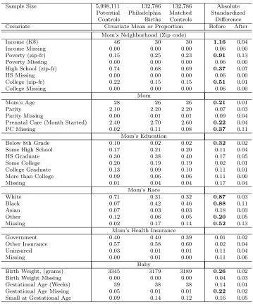
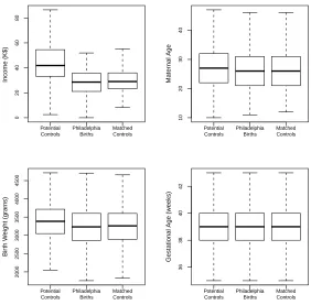
The third part of the thesis is an application of the split samples method to an observational study on the effect of obstetric unit closures in Philadelphia. The splitting was successful twice over: (i) it successfully identified an interesting and moderately insensitive conclusion, (ii) by comparison of the planning and analysis samples, it is clearly seen to have avoided an exaggerated claim of insensitivity to unmeasured bias that might have occurred by focusing on the least sensitive of many findings. Under the assumption of no unmeasured confounding, we found strong evidence that obstetric unit closures caused birth injuries. We also showed this conclusion to be insensitive to bias from a moderate amount of unmeasured confounding.
Degree Type
Dissertation
Degree Name
Graduate Group
Statistics
First Advisor
Lawrence D. Brown
Keywords
Causal Inference, Design Sensitivity, High-dimensional Inference, Linear Regression, Model Selection, Multiple Comparison
Subject Categories
VALID POST-SELECTION
INFERENCE
Kai Zhang
A DISSERTATION
in
Statistics
For the Graduate Group in Managerial Science and Applied
Economics
Presented to the Faculties of the University of Pennsylvania
in
Partial Fulfillment of the Requirements for the
Degree of Doctor of Philosophy
2012
Supervisor of Dissertation
Lawrence D. Brown, Miers Busch Professor, Statistics
Graduate Group Chairperson
Eric Bradlow, K.P. Chao Professor, Marketing, Statistics and Education
Dissertation Committee
Lawrence D. Brown, Miers Busch Professor, Statistics
Andreas Buja, The Liem Sioe Liong/First Pacific Company Professor, Statistics Edward I. George, Universal Furniture Professor, Statistics
VALID POST-SELECTION INFERENCE
COPYRIGHT
2012
Kai Zhang
This work is licensed under the Creative Commons
Attribution-NonCommercial-ShareAlike 3.0 License
To view a copy of this license, visit
Acknowledgement
My sincere gratitude goes to my family, all my teachers, and all my friends for
their love and support over the past few years.
I am indebted to my thesis advisor Professor Lawrence D. Brown for his fatherly
nurturing and guidance. His thinking is always extremely sharp and deep that
in-spires me to think further. His advice is always extremely insightful and helpful that
stimulates me to work harder. He is also extremely patient and considerate to give
me many warm encouragements that helps me to overcome difficulties. Although
scientific research is never easy, Professor Brown is always my source of courage and
power.
I thank my thesis committee members Professors Andreas Buja, Edward I. George,
Dylan S. Small, and Linda Zhao for their kind and careful supervision. They
provid-ed me both deep understanding of the theories and fundamental tools in research.
They also gave me very generous support in the past five years.
I am grateful to my collaborators Sathyanarayan Anand, Richard Berk, Dean
Foster, Ruth Heller, Hongzhe Li, Scott Lorch, Zongming Ma, James Piette, Emil
Pitkin, Alexander Rakhlin, Paul Rosenbaum, Jeffrey Silber, Sindhu Srinivas, and
Mikhail Traskin, and instructors Tony Cai, Warren Ewens, Shane Jensen, Abba
Steele, Robert Stine, Jessica Wachter, and Abraham Wyner. The inspiration and
education I received from them will benefit my entire career.
Many thanks to the staff members Adam Greenberg, Daniel Huang, Catharina
LeBlanc, Carol Reich, Andrew Romond, Sarin Sieng, Anand Srinivasan, Debbie
Todd, and Tanya Winder for creating excellent environment for me to study here.
I would like to thank my colleague students. My years of graduate study here
would not have been this colorful without them.
My final, and most heartfelt, acknowledgment must go to my family. This
disser-tation would not have been possible without their unconditional love and support.
ABSTRACT
VALID POST-SELECTION INFERENCE
Kai Zhang
Lawrence D. Brown
In the classical theory of statistical inference, data is assumed to be generated from
a known model, and the properties of the parameters in the model are of interest.
In applications, however, it is often the case that the model that generates the data
is unknown, and as a consequence a model is often chosen based on the data. In
my dissertation research, we study how to achieve valid inference when the model
or hypotheses are data-driven. We study three scenarios, which are summarized in
the three chapters.
In the first chapter, we study the common practice to perform data-driven
vari-able selection and derive statistical inference from the resulting model. We find
such inference enjoys none of the guarantees that classical statistical theory
pro-vides for tests and confidence intervals when the model has been chosen a priori.
We propose to produce valid “post-selection inference” by reducing the problem to
one of simultaneous inference. Simultaneity is required for all linear functions that
arise as coefficient estimates in all submodels. By purchasing “simultaneity
universally valid under all possible model selection procedures. This inference is
therefore generally conservative for particular selection procedures, but it is always
more precise than full Scheff´e protection. Importantly it does not depend on the
truth of the selected submodel, and hence it produces valid inference even in wrong
models. We describe the structure of the simultaneous inference problem and give
some asymptotic results.
In the second chapter of this thesis, we propose a different approach to achieve valid
post-selection inference which corresponds to the treatment of the design matrix
predictors as random. Our methodology is based on two techniques, namely split
samples and the bootstrap. Split-sample methodology generally involves dividing
the observations randomly into two parts: one part for exploratory model building,
a.k.a. the training set or planning sample, and the other part for confirmatory
statistical inference, a.k.a. holdout set or analysis sample. We use a training sample
only to seek a subset of predictors, and then perform the estimation and inference
on the holdout set. As far as inference after selection in linear models is concerned,
the main advantage of this technique is, roughly speaking, that it separates the data
for exploratory analysis from the data for confirmatory analysis, thereby removing
the contaminating effect of selection on inference. We show that the our procedure
achieves valid inference asymptotically for any selection rule.
The third part of the thesis is an application of the split samples method to an
observational study on the effect of obstetric unit closures in Philadelphia. The
splitting was successful twice over: (i) it successfully identified an interesting and
samples, it is clearly seen to have avoided an exaggerated claim of insensitivity to
unmeasured bias that might have occurred by focusing on the least sensitive of
many findings. Under the assumption of no unmeasured confounding, we found
strong evidence that obstetric unit closures caused birth injuries. We also showed
this conclusion to be insensitive to bias from a moderate amount of unmeasured
Contents
Dedication . . . iii
Acknowledgement . . . iv
Abstract . . . vi
List of Tables . . . xiii
List of Figures . . . xiv
Preface . . . xv
1 The PoSI Approach 1 1.1 Introduction — The Problem with Statistical Inference after Model Selection . . . 1
1.2 Model Selection Re-Interpreted . . . 5
1.2.1 Post-Selection Inference for Full Model Parameters — a Dead End . . . 5
1.2.2 The Meaning of Regression Coefficients . . . 8
1.2.3 Assumptions, “Wrong Models”, and Error Estimates . . . 12
1.3 Estimation and its Targets in Submodels . . . 15
1.3.1 Multiplicity of Regression Coefficients . . . 15
1.3.2 “Omitted Variables Bias” . . . 18
1.3.3 Interpreting Regression Coefficients in First-Order Incorrect Models . . . 19
1.4 Universally Valid Post-Selection Confidence Intervals . . . 20
1.4.1 Test Statistics with One Error Estimate for All Submodels . . 20
1.4.2 Model Selection and Its Implications for Parameters . . . 22
1.4.4 Universal Validity for all Selection Procedures . . . 24
1.4.5 Restricted Model Selection . . . 26
1.4.6 Reduction of Universally Valid Post-Selection Inference to Si-multaneous Inference . . . 28
1.4.7 Scheff´e Protection . . . 30
1.4.8 PoSI-Sharp Model Selection — “SPAR” and “SPAR1” . . . . 32
1.4.9 PoSI P-Value Adjustment for Model Selection . . . 34
1.5 The Structure of the PoSI Problem . . . 36
1.5.1 Canonical Coordinates . . . 36
1.5.2 PoSI Coefficient Vectors in Canonical Coordinates . . . 37
1.5.3 Orthogonalities of PoSI Coefficient Vectors . . . 38
1.5.4 The PoSI Process . . . 40
1.5.5 The PoSI Polytope . . . 41
1.5.6 PoSI Optimality of Orthogonal Designs . . . 42
1.5.7 A Duality Property of PoSI Vectors . . . 45
1.6 Illustrative Examples and Asymptotic Results . . . 47
1.6.1 Example 1: The PoSI Problem for Exchangeable Designs . . . 47
1.6.2 Example 2: Where K(X) is close to the Scheff´e Bound . . . . 50
1.6.3 Bounding Away from Scheff´e . . . 52
2 The Split Samples Approach 55 2.1 Introduction . . . 55
2.1.1 Split Samples . . . 56
2.1.2 Random Design View . . . 57
2.1.3 Nonlinearity and Bootstrap . . . 58
2.2 Population . . . 60
2.3 Valid Inference in the Full Model . . . 64
2.3.1 Least Squares Estimates in the Full Model . . . 64
2.3.2 Bootstrap Inference for LS Estimates in the Full Model . . . . 66
2.4 Valid Post-Selection Inference via Split Samples and Bootstrap . . . . 69
2.4.1 Least Squares Estimates in A Submodel . . . 69
2.4.2 Valid Bootstrap Inference under A Submodel . . . 71
2.4.3 A Split Samples Procedure . . . 72
2.5 Inference under First-Order Correctness and Homoscedasticity . . . . 74
2.5.1 The Properties of LS Estimates under First-Order Correctness and Homoscedasticity . . . 75
2.5.3 Valid Bootstrap Inference in Submodels under the Gaussian
Distribution . . . 78
3 Using Split Samples in an Observational Study 79 3.1 Introduction: background; methodological outline . . . 79
3.1.1 A wave of closures of hospital obstetrics units . . . 79
3.1.2 Matching to build a control Philadelphia . . . 81
3.1.3 Splitting . . . 86
3.1.4 Evidence factors . . . 89
3.2 Matching . . . 91
3.2.1 Philadelphia and elsewhere, before and after matching . . . . 91
3.2.2 How the matching was done . . . 95
3.3 Splitting . . . 97
3.3.1 A 10%-90% random split for design and analysis . . . 97
3.3.2 Birth injury in the planning sample: the largest difference, two nearly independent tests for effect and a test for unmeasured bias . . . 99
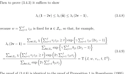
3.4 Observational studies with binary outcome and difference-in-differences104 3.4.1 Notation: base and intervention periods; exposed and unex-posed regions . . . 104
3.4.2 Model for sensitivity analysis . . . 105
3.4.3 Sensitivity analysis with binary outcomes in difference-in-differences analysis . . . 109
3.5 Confirmatory analysis using the 90% sample . . . 113
4 Conclusion and Discussion 119 4.1 Conclusion and Discussion of the PoSI Approach . . . 119
4.2 Conclusion and Discussion of the Split Samples Approach . . . 121
4.3 Conclusion and Discussion of the Real Data Application of the Split Samples Method . . . 123
4.4 Thoughts about Future Research . . . 124
A Appendix 125 A.1 Proofs in Chapter 1 . . . 125
A.1.1 Proof of Theorem 1.4.3 . . . 125
A.1.2 Proof of Proposition 1.5.3 . . . 127
A.1.3 Proof of Duality: Lemma 1.5.1 and Theorem1.5.1 . . . 127
A.1.5 Proof of Theorem 1.6.2 . . . 132 A.1.6 Proof of Theorem 1.6.3 . . . 135
List of Tables
3.1 Covariate balance before and after matching . . . 84 3.2 Results for birth injury in the planning component of the split sample 100 3.3 General form of the table under H0 . . . 111
List of Figures
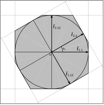
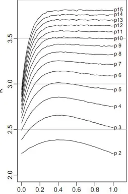
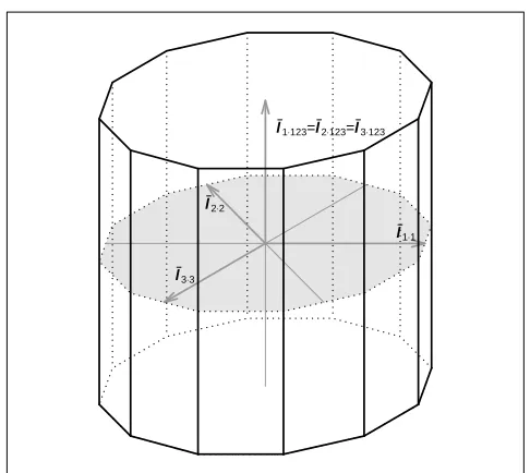
1.1 The PoSI polytope for d=p= 2 . . . 43 1.2 The PoSI constant K(X, α = 0.05) for exchangeable designs . . . 48 1.3 The geometry of the limiting PoSI polytope forp= 3 for exchangeable
designs . . . 51
2.1 The decomposition of Y when p= 1. . . 62
Preface
In a series of papers, John Tukey (1980a; 1980b) envisioned the future of statistics
by distinguishing two important aspects: exploratory data analysis and
confirmato-ry data analysis. Indeed, in many modern applications of statistics, data analyses
are guided by both of the following ideas: (1) People want to understand the
mech-anism in the data with a parsimonious model. This model is to be found through
some data-driven model selection; and (2) People want to make valid statistical
inference from the model they select. In light of these ideas, I have been working
on methodologies that achieve valid inference after model selection. My work is
summarized in the three parts of this dissertation.
The first part of this thesis is based on the paper Valid Post-Selection Inference
(2012) which is a joint work with Richard Berk, Lawrence Brown, Andreas Buja,
and Linda Zhao. The second part of this thesis is based on a paper in
prepara-tion that will be a joint work with Richard Berk, Lawrence Brown, Andreas Buja,
Edward George, Emil Pitkin, Mikhail Traskin, and Linda Zhao. The third part of
this thesis is based on the paper Using Split Samples and Evidence Factors in an
Observational Study of Neonatal Outcomes (2011) which is a joint work with Scott
Lorch, Paul Rosenbaum, Dylan Small, and Sindhu Srinivas. I am very thankful for
to Lawrence Brown, Andreas Buja, Paul Rosenbaum, and Dylan Small for their
Chapter 1
The PoSI Approach
1.1
Introduction — The Problem with Statistical
Inference after Model Selection
Classical statistical theory grants validity of statistical tests and confidence intervals
assuming a wall of separation between the selection of a model and the analysis of
the data being modeled. In practice, this separation rarely exists and more often a
model is “found” by a data-driven selection process. As a consequence inferential
guarantees derived from classical theory are invalidated. Among model selection
methods that are problematic for classical inference, variable selection stands out
because it is regularly taught, commonly practiced, and highly researched as a
tech-nology. Even though statisticians may have a general awareness that the data-driven
selection of variables (predictors, covariates) must somehow affect subsequent
pervasive that it appears in classical undergraduate textbooks on statistics such as
Moore and McCabe (2003).
The reason for the invalidation of classical inference guarantees is that a
data-driven variable selection process produces a model that is itself stochastic, and this
stochastic aspect is not accounted for by classical theory. Models become stochastic
when the stochastic component of the data is involved in the selection process. (In
regression with fixed predictors the stochastic component is the response.) Models
are stochastic in a well-defined way when they are the result of formal variable
selection procedures such as stepwise or stagewise forward selection or backward
elimination or all-subset searches driven by complexity penalties (such as Cp, AIC,
BIC, risk-inflation, LASSO, ...) or prediction criteria such as cross-validation, or
recent proposals such as LARS and the Dantzig selector (for an overview see, for
example, Hastie, Tibshirani, and Friedman (2009)). Models are also stochastic but
in an ill-defined way when they are informally selected through visual inspection of
residual plots or normal quantile plots or generally through activities that may be
characterized as “data snooping”. Finally, models become stochastic in the most
opaque way when their selection is affected by human intervention based on post hoc
considerations such as “in retrospect only one of these two variables should be in the
model” or “it turns out the predictive benefit of this variable is too weak to warrant
the cost of collecting it.” In practice, all three modes of variable selection may be
exercised in the same data analysis: multiple runs of one or more formal search
algorithms may be performed and compared, the parameters of the algorithms may
diagnostics; a round of fine-tuning based on substantive deliberations may finalize
the analysis.
Posed so starkly, the problems with statistical inference after variable selection
may well seem insurmountable. At a minimum, one would expect technical solutions
to be possible only when a formal selection algorithm is (1) well-specified (1a) in
advance and (1b) covering all eventualities, (2) strictly adhered to in the course of
data analysis, and (3) not “improved” on by informal and post-hoc elements. It may,
however, be unrealistic to expect this level of rigor in most data analysis contexts,
with the exception of well-conducted clinical trials. The real challenge is therefore
to devise statistical inference that is valid following any type of variable selection, be
it formal, informal, post hoc, or a combination thereof. Meeting this challenge with
a relatively simple proposal is the goal of this article. This proposal for valid Po
st-SelectionInference, or “PoSI” for short, consists of a large-scale family-wise error
guarantee that can be shown to account for all types of variable selection, including
those of the informal and post-hoc varieties. On the other hand, the proposal is no
more conservative than necessary to account for selection, and in particular it can
be shown to be less conservative than Scheff´e’s simultaneous inference.
The framework for our proposal is in outline as follows — details to be
elabo-rated in subsequent sections: We consider linear regression with predictor variables
whose values are considered fixed, and with a response variable that has normal
and homoscedastic errors. The framework does not require that any of the eligible
linear models is correct, not even the full model, as long as a valid error estimate
that makes use of the response, but the procedure does not need to be fully
speci-fied. A crucial aspect of the framework concerns the use and interpretation of the
selected model: We assume that, after variable selection is completed, the selected
predictor variables — and only they — will be relevant; all others will be
eliminat-ed from further consideration. This assumption, seemingly innocuous and natural,
has critical consequences: It implies that statistical inference will be sought for the
coefficients of the selected predictors only and in the context of the selected model
only. Thus the appropriate targets of inference are the best linear coefficients within
the selected model, where each coefficient is adjusted for the presence of all other
included predictors but not those that were eliminated. Therefore the coefficient
of an included predictor generally requires inference that is specific to the model
in which it appears. Summarizing in a motto, a difference in adjustment implies a
difference in parameters and hence in inference. The goal of the present proposal is
therefore simultaneous inference for all coefficients in all submodels. Such inference
can be shown to be valid following any variable selection procedure, be it formal,
informal, post hoc, fully or only partly specified.
Problems associated with post-selection inference were recognized long ago, for
ex-ample, by Buehler and Fedderson (1963), Brown (1967), Olshen (1973), Sen (1979),
Sen and Saleh (1987), Dijkstra and Veldkamp (1988), P¨otscher (1991), Kabaila
(1998). More recently these problems have been the subject of incisive analyses by
Leeb and P¨otscher (2003; 2005; 2006a; 2006b; 2008a; 2008b), Kabaila and Leeb
(2006), Leeb (2006), and P¨otscher and Leeb (2009).
difficulties of post-selection inference as they transpire from the work of Leeb and
P¨otscher cited above (Section 1.2.1); we then rethink the assumptions
underly-ing their analyses and lay some groundwork by proposunderly-ing new (or old) meanunderly-ings
for regression coefficients (Section 1.2.2); we conclude the section by discussing
as-sumptions with a view towards valid inference in “wrong models” (Section 1.2.3).
Section 1.3 is about estimation and its targets; Section 1.4 develops the
methodol-ogy for PoSI confidence intervals (CIs) and tests. After some structural results for
the PoSI problem in Section 1.5 , we show in Section 1.6 that with increasing
num-ber of predictors p the width of PoSI CIs can range between the asymptotic rates
O(√logp) and O(√p). We give examples for both rates and, inspired by problems
in sphere packing and covering, we give upper bounds for the limiting constant in
the O(√p) case. Some proofs are deferred to the appendix.
1.2
Model Selection Re-Interpreted
1.2.1
Post-Selection Inference for Full Model Parameters —
a Dead End
It is a natural intuition that model selection distorts inference by distorting
sam-pling distributions of parameter estimates: One expects that estimates in selected
models tend to generate more Type I errors than conventional theory would
sug-gest because the typical selection procedure favors models with strong, hence highly
which would tend to become more severe as the number of predictors subject to
se-lection increases. This problem will be addressed here with a simultaneous inference
approach.
A second problem with inference after model selection is pointed out by Leeb and
P¨otscher in the above referenced series of articles. The problem exists even in a
two-predictor situation, as illustrated by Leeb and P¨otscher (2005): They analyze a
case with a predictor that is protected from selection and a covariate that is subject
to selection, and they provide an explicit finite-sample formula for the sampling
distribution of the coefficient estimate of the protected predictor, as the covariate is
randomly selected/deselected according to a BIC-equivalent test to grant consistent
model selection (ibid., p. 29). The analysis reveals in graphic ways (ibid., Figure 2)
that the sampling distribution depends critically on the unknown true coefficient of
the covariate and the sample size, with egregious deviations from the fixed-model
sampling distribution ranging from bi-modality to approximate normality with
in-flated variance. Because the true covariate slope is not known, there is no way of
determining whether the sample size places the sampling distribution in this realm
of deviation from classical theory.
Generalizing to arbitrary linear models Leeb and P¨otscher (2003; 2005; 2006a;
2006b; 2008a; 2008b) show that sampling distributions cannot be estimated after
model selection, not even asymptotically. Ironically, the asymptotics that describe
the devious finite sample behavior of sampling distributions best are those based on
consistent model selection. They show that asymptotic normality is riddled with
when telescoping true slopes to zero so as to approach submodels. Leeb and P¨otscher
(2005, p. 27) arrive at the following conclusion: “the post-model-selection estimator
... is nothing else than a variant of Hodges’ so-called superefficient estimator.”
It is little comfort that these problems are non-existent for perfectly orthogonal
regression designs (Leeb and P¨otscher 2005, p. 43f). In the majority of practical
contexts there is some degree of collinearity, and one of the purposes of model
selection is to weed out predictor redundancies caused by partial collinearity. Leeb
and P¨otscher’s analysis is compelling within their framework, but the intractable
situation they expose suggests a need to renegotiate the assumptions that underlie
their framework.
Leeb and P¨otscher (ibid.), like many authors in this area, make the fundamental
assumption that all estimation is in the full model. Thus, if a model selection
procedure excludes a predictor, this is interpreted as forcing the estimate of its
slope to zero. Consequently, a slope estimate ˆβj of a predictor is always defined,
whether it is selected or not: ˆβj is the LS estimate in the selected submodel if the
jth predictor is included, and it is zero otherwise. Either way, the resulting value is
interpreted as an estimate of βj in the full model. A parallel consequence is that in
this interpretation the coefficient of a predictor has always the same meaning as a
full-model parameter, irrespective of which covariates are selected or excluded. It is
under this framework that post-selection estimators can be interpreted as generalized
superefficient Hodges estimators with the ensuing problems of non-uniformity (Leeb
and P¨otscher 2005). This problem can also be seen as an inferential analog of the
Angrist and Pischke 2009).
1.2.2
The Meaning of Regression Coefficients
Our solution to the inferential problem associated with “omitted variables bias” is
to assert that submodels have their own separate parameters, and it is these that
are being estimated in the selected submodels. We start the discussion with the
following questions:
(1) When we select submodels in practice, do we think of excluded predictors as
having a zero slope?
(2) Does the full model necessarily have special status?
(3) Can a slope estimate be interpreted as estimating the same target parameter,
regardless of what the other predictors are?
The short answers are:
(1) The slopes of excluded predictors are not zero; they are not defined and
there-fore don’t exist.
(2) The full model has no special status.
(3) The meaning of a slope depends on which predictors are included in the
se-lected model.
As for (1), assigning a zero value to predictors that are not in the model is an
elegant technical device, but it is not something that describes how we think or
even how we should think about slopes and their estimates. The PoSI framework
we describe in Section 1.3 will not require zero slope fill-ins.
As for (2), the full model cannot be argued to have generally special status because
there is generally a question of predictor redundancy. It is a common experience that
models are proposed on theoretical grounds but found on empirical grounds to have
their predictors hopelessly entangled by collinearities that permit little meaningful
statistical inference. This is best illustrated with a concrete example (inspired by
Mosteller and Tukey (1977), p. 326f): Consider a study of performance of students
in a large school system. Interested in socio-economic factors, investigators wish to
pin down the predictors that are most strongly associated with children’s success
in school: father’s and mother’s highest education levels, their high school GPAs,
their SAT scores, their frequencies of intensive reading, the perceived importance
they each assign to education, and so on. There should be little surprise that, if all
these predictors are included in the model, the overall test rejects but none of the
individual predictors is statistically significant. Informal model selection, however,
may show that each predictor is highly statistically significant if retained alone in
the model. The obvious reason is that these predictors measure essentially the same
trait in parents, hence are highly collinear with each other. As a consequence, the
full model is not viable in the first place. This situation is not limited to the social
sciences: in gene expression studies it may well occur that numerous sites have a
will be hopelessly confounded. The bias in favor of full models may be particularly
strong in econometrics where there is a “notion that a longer regression ... has a
causal interpretation, while a shorter regression does not” (Angrist and Pischke 2009,
p. 59). Even in causal models, however, there is a possibility that included adjustor
variables will “adjust away” some of the causal variables of interest. Generally, in any
creative observational study involving novel predictors it will be difficult to exclude
surprising collinearities that might force a rethinking of the role of predictors. In
conclusion, whenever predictor redundancy is a potential issue, it cannot a priori be
claimed that the full model provides the parameters of primary interest.
As for (3), we do teach that the meaning of a slope depends on what other
pre-dictors are included in the chosen model: “the slope is the average difference in the
response for a unit difference in the predictor, at fixed levels of all other predictors.”
This last condition is sometimes rendered as “adjusted for all other predictors” and
called the “Ceteris Paribus” clause (see, for example, Angrist and Pischke 2009). It
is an essential part of the meaning of a slope. That there is a difference in meaning
when there is a difference in covariates is most drastically evident when there is
a case of Simpson’s paradox. This is again best illustrated with a concrete
exam-ple: A company is introducing a new high-tech device and conducts a consumer
survey that includes a response for self-reported purchase likelihood (P L), as well
as two predictors, Age and Income. We consider a model with Age alone and one
with both Age andIncome. [Note that the smaller model cannot be disregarded as
“wrong”. IfIncome is difficult to measure, it may be useful to rely on the equation
linear submodel is “correct”.] Now, it is sensibly anticipated that younger
respon-dents will rate themselves with higher P L, but a regression of P L on Age alone
produces a significantly positive slope estimate, indicating that older respondents
have higher P L. On the other hand, a regression of P L on both Age and Income
yields a significantly negative slope estimate forAge, indicating that,comparing only
respondents at the same Income level, younger respondents have indeed higherP L.
This instance of Simpson’s paradox is enabled by a positive collinearity betweenAge
and Income that turns Age into a proxy for Income. Must we use the full model?
Not if the improvement in R2 is practically irrelevant even though Income is
sta-tistically significant (apart from the issue of availability of Income measurements).
Is the marginal slope of P L on Age an estimate of the Income-adjusted slope on
Age? Certainly not — the two slopes answer very different questions, apart from
having opposite signs. In conclusion, differences in adjustment result in different
parameters.
From these considerations follows a framework in which the full model is no longer
the sole provider of parameters, where rather each submodel defines its own. The
consequences of this view will be elaborated in Section 1.3.
In the preceding discussions we assumed a focus on the interpretation of the
se-lected submodel and hence on inference for its coefficients. When the focus is on
prediction, on the other hand, the focus is on predicted values. Yet, even in
predic-tion problems there is sometimes a quespredic-tion of which predictors matter most within
a selected submodel, and here a suitable t-statistic of a coefficient estimate is a
predictors in the submodel. In this context the submodel-specific parameters are
the appropriate ones to consider.
1.2.3
Assumptions, “Wrong Models”, and Error Estimates
We state assumptions for estimation and for the construction of valid tests and CIs.
A major goal is to prepare the ground for valid statistical inference after model
selection in “first order wrong models”.
We consider a quantitative response vector Y∈Rn, assumed random, and a full
predictor matrix X = (X1,X2, . . . ,Xp)∈ Rn×p, assumed fixed. We allow X to
be of non-full rank, and n and p to be arbitrary. In particular, we allow n < p.
Throughout the article we let
d , rank(X) = dim(span(X)), hence d≤min(n, p). (1.2.1)
Due to frequent reference we call d=p(≤n) “the classical case”.
It is common practice to assume the full model Y∼ Nn(Xβ, σ2I) to be correct.
In the present framework, however, first-order correctness, E[Y] = Xβ, will not
be assumed. By implication, first-order correctness of any submodel will not be
assumed either. Effectively,
µ , E[Y]∈Rn (1.2.2)
is allowed to be unconstrained and, in particular, need not reside in the column space
ofX. In other words, the model given byXis allowed to be “first-order wrong”, and
he calls “wrong models”, however, we prefer to call “approximations”: All predictor
matrices X provide approximations to µ, some better than others, but the degree
of approximation plays no role in the clarification of statistical inference. We will
echo Box as follows: all models are mere approximations, yet some are useful. The
main reason for elaborating this point is as follows: after model selection the case
for “correct models” is clearly questionable, even for “consistent model selection
procedures” (Leeb and P¨otscher 2003, p. 101); but if correctness of submodels is
not assumed, it is only natural to abandon this assumption for the full model also,
in line with the idea that the full model has no special status. As we proceed with
estimation and inference guarantees in the absence of first-order correctness we will
rely on assumptions as follows:
• For estimation (Section 1.3), we will only need the existence of µ=E[Y].
• For testing and CI guarantees (Section 1.4), we will make conventional second
order and distributional assumptions:
Y ∼ N(µ, σ2I). (1.2.3)
The assumptions (1.2.3) of homoscedasticity and normality are as questionable as
first order correctness, and we will report elsewhere on approaches that avoid them.
In the present work, we choose to follow the large model selection literature that
relies on the technical advantages of assuming homoscedastic and normal errors.
Accepting the assumption (1.2.3), we address the issue of estimating the error
of σ2 that is independent of LS estimates. In the classical case, the most common
way to assert such an estimate is to assume that the full model is first order correct,
µ=Xβ in addition to (1.2.3), in which case the mean squared error (MSE), ˆσ2
F =
kY −X ˆβk2/(n − p), of the full model will do. However, other possibilities for
producing a valid estimate ˆσ2 exist, and they may allow relaxing the assumption of
first order correctness:
• Exact replications of the response obtained under identical conditions might
be available in sufficient numbers. An estimate ˆσ2 can be obtained as the MSE
of the one-way ANOVA of the groups of replicates.
• In general, a larger linear model than the full model might be considered as
correct, hence ˆσ2 could be the MSE from this larger model.
• A different possibility is to use another dataset, similar to the one currently
being analyzed, to produce an independent estimate ˆσ2 by whatever valid
estimation method.
• A special case of the preceding is a random split-sample approach whereby one
part of the data is reserved for producing ˆσ2 and the other part for estimating
coefficients, selecting models, and carrying out post-model selection inference.
• A very different type of estimates ˆσ2may be based on considerations borrowed
from non-parametric function estimation (Hall and Carroll 1989).
The purpose of pointing out these possibilities is to separate at least in principle
the issue of first-order model incorrectness from the issue of valid and independent
within our framework as the valid and independent estimation of σ2 is a problem
faced by all “n < p” approaches.
1.3
Estimation and its Targets in Submodels
Following Section 1.2.2, the meaning and numeric value of a regression coefficient
depends on what the other predictors in the model are. This statement requires a
qualification: it assumes that the predictors are non-orthogonal/partially collinear.
If they are perfectly pairwise orthogonal, as in some designed experiments or in
function fitting with orthogonal basis functions, a coefficient has the same identity
across all submodels, both in meaning and in value, because adjustment of predictors
for each other and the ceteris paribus clause become vacuous. This article is hence
largely a story of (partial) collinearity.
1.3.1
Multiplicity of Regression Coefficients
We will give meaning to LS estimators and their targets in the absence of any
assumptions other than the existence ofµ=E[Y], which in turn is permitted to be
entirely unconstrained inRn. Besides resolving the issue of estimation in “first order
wrong models”, the major point here is to follow up on the idea that the regression
coefficient of a predictor generates different parameters in different submodels. As
each predictor appears in 2p−1 submodels, the p regression coefficients of the full
model generally proliferate into a plethora of as many as p2p−1 distinct regression
start with notation.
To denote a submodel we use the (non-empty) index set M = {j1, j2, ..., jm} ⊂
MF ={1, . . . , p} of the predictors Xji in the submodel; the size of the submodel is
m = |M| and that of the full model is p = |MF|. Let XM = (Xj1, ...,Xjm) denote
the n×m submatrix of X with columns indexed by M. We will assume that only
submodels M are considered for which XM is of full rank:
rank(XM) = m ≤ d.
We let βˆM be the unique least squares estimate in M:
ˆ
βM= (XTMXM)−1XTMY. (1.3.1)
Now thatβˆMis an estimate, what is it estimating? A conclusion from Section 1.2.1
is that βˆM does not estimate the coefficients in the full model. Because any larger
model could have been the full model, we generalize by asserting that βˆM does not
estimate parameters in any other model than M itself. In M, it is natural to ask
that βˆM be an unbiased estimate of its target:
βM , E[βˆM] = (XTMXM)−1XTME[Y] (1.3.2)
= argmin
β0∈
Rm
kµ−XMβ0k2
This definition requires only the existence of µ=E[Y] but no other assumptions.
does it matter to what degree M provides a good approximation to µ in terms of
approximation errorkµ−XMβMk2. Asserting that the model M is “correct” would
mean µ∈span(XM) or equivalently the approximation error vanishes; in this case
βM would be the “true” parameter.
In the classical cased=p≤n, we can define the target of the full-model estimate
ˆ
β = (XTX)−1XTY as a special case of (1.3.2) with M = M F:
β , E[βˆ] = (XTX)−1XTE[Y]. (1.3.3)
In the general (non-classical) case, let β be any (possibly non-unique) minimizer of
kµ−Xβ0k2; the link betweenβ and β
M is as follows:
βM = (XTMXM)−1XTMXβ. (1.3.4)
Thus the target βM is an estimable linear function of β, without any first-order
assumptions. Equation (1.3.4) follows from span(XM)⊂span(X).
Notation: To distinguish regression coefficients as a function of the model they
appear in, we write βj·M = E[ ˆβj·M] for the components of βM =E[βˆM] with j∈M.
An important convention we adopt throughout this article is that the index j of
a coefficient refers to the coefficient’s index in the original full model MF: βj·M
for j ∈ M refers not to the j’th coordinate of βM, but to the coordinate of βM
corresponding to the j’th predictor Xj in the full predictor matrix X. We refer to
1.3.2
“Omitted Variables Bias”
By allowing each ˆβj·M to estimate its own target βj·M and thereby relieving ˆβj·M of
the burden of estimating the parameterβj in the full model, we sidestep the problem
of “omitted variables bias” and with it a major driver of the problems analyzed by
Leeb and P¨otscher (Section 1.2.1). In the present framework βj−βj·M is not a bias
as these are two different parameters that answer two different questions. Just the
same, we consider briefly the difference between βj and βj·M in the classical case
d=p≤n. Compare the following two definitions:
βM ,E[βˆM] and βM,(βj)j∈M, (1.3.5)
the latter being the coefficientsβj from the full model MF subsetted to the
submod-el M. While βˆM estimates βM, it does not generally estimate βM. The difference
βM−βM is the vectorized “omitted variables bias”.
In general, the definition of βM involves X and all of β, not just βM, through
(1.3.4). A little algebra shows that βM =βM if and only if
XTMXMcβM c
=0, (1.3.6)
where Mcdenotes the complement of M in the full model M
F. Special cases of (1.3.6)
include: (1) the column space ofXMis orthogonal to that ofXMc, and (2)βM c
=0,
meaning that the approximation to µ in MF is no better than in M, or if the full
1.3.3
Interpreting Regression Coefficients in First-Order
In-correct Models
The regression coefficient βj·M is conventionally interpreted as the “average
dif-ference in the response for a unit difdif-ference in Xj, ceteris paribus in the
mod-el M”. This interpretation no longer holds when the assumption of first order
correctness is given up. Instead, the phrase “average difference in the response”
should be replaced with the unwieldy but more correct phrase “average
differ-ence in the response approximated in the submodel M”. The reason is that the
fit in the submodel M is ˆYM = HMY (HM = XM(XTMXM)−1XTM) whose target
is µM = E[ ˆYM] = HME[Y] = HMµ. Thus in the submodel M we estimate not
the true µ but the LS approximation µM to µ using XM: µM = XMβM, where
βM= argminβ0kµ−XMβ0k2.
A second interpretation of regression coefficients is in terms of adjusted
predic-tors: For j ∈ M define the M-adjusted predictor Xj·M as the residual vector of
the regression of Xj on all other predictors in M. Multiple regression coefficients,
both estimates ˆβj·M and parameters βj·M, can be expressed as simple regression
coefficients with regard to the M-adjusted predictor:
ˆ βj·M =
XT j·MY
kXj·Mk2
, βj·M =
XT j·Mµ
kXj·Mk2
. (1.3.7)
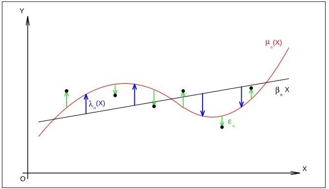
The left hand formula lends itself to an interpretation of ˆβj·M in terms of the
well-known leverage plot which shows Y plotted against Xj·M and the line with slope
ˆ
A third interpretation can be derived from the second: For notational reasons
let x = (xi)i=1...n be any adjusted predictor Xj·M, so that ˆβ = xTY/kxk2 and
β = xTµ/kxk2 are the corresponding ˆβ
j·M and βj·M. Introduce case-wise slopes
through the origin, both as estimates ˆβ(i) = Yi/xi and as parameters β(i) = µi/xi,
as well as case-wise weights w(i) = x2i/
P
i0=1...nx2i0. Equations (1.3.7) are then
equivalent to the following:
ˆ
β = X
i
w(i)βˆ(i), β = X
i
w(i)β(i).
Hence regression coefficients are weighted averages of case-wise slopes, and this
interpretation holds without first-order assumptions.
1.4
Universally Valid Post-Selection Confidence
Intervals
1.4.1
Test Statistics with One Error Estimate for All
Sub-models
After defining βM as the target of the estimate βˆM, we consider inference for it in
terms of test statistics. Following Section 1.2.3 we require a normal homoscedastic
have equivalently
ˆ
βM ∼ N(βM, σ2(XTMXM)−1) and βˆj·M∼ N(βj·M, σ2/kXj·Mk2).
Again following Section 1.2.3 we assume the availability of a valid estimate ˆσ2 ofσ2
that is independent of all estimates ˆβj·M, and we further assume ˆσ2 ∼ σ2χ2r/r for r
degrees of freedom. If the full model is assumed correct, n > p and ˆσ2= ˆσ2
F, then
r =n−p. In the limit r→ ∞ we obtain ˆσ =σ, the case of known σ, which will be
used starting with Section 1.6.
Let tj·M denote a t-ratio for βj·M that uses ˆσ irrespective of the submodel M:
tj·M ,
ˆ
βj·M−βj·M
((XT
MXM)−1)
1 2
jj σˆ
= ˆ
βj·M−βj·M
ˆ
σ/kXj·Mk
= (Y−µ)
TX
j·M
ˆ
σkXj·Mk
. (1.4.1)
[According to full model indexing, (...)jjrefers to the diagonal element corresponding
to Xj.] The quantity tj·M = tj·M(Y) has a central t-distribution with r degrees of
freedom. Essential is that the standard error estimate in the denominator of (1.4.1)
does notinvolve the MSE ˆσM from the submodel M, for two reasons:
• We do not assume that the submodel M is first-order correct; therefore each
MSE ˆσ2
M could have a distribution that is a multiple of a non-central χ2
dis-tribution with unknown non-centrality parameter.
• More disconcertingly, the MSE would be the result of selection: ˆσM2ˆ. Not much
of real use is known about its distribution (see, for example, Brown 1967 and
These problems are avoided by using one valid estimate ˆσ2 that is independent of
all submodels.
With this choice of ˆσ, a marginal 1−α confidence interval for βj·M is
CIj·M(K) , h
ˆ
βj·M ± K
(XTMXM)−1 12
jj σˆ
i
(1.4.2)
= hβˆj·M ± Kσ/ˆ kXj·Mk i
.
where K = tr,1−α/2 is the 1−α/2 quantile of a t-distribution with r degrees of
freedom. This interval is valid, that is,
P[βj·M∈CIj·M(K)] ≥ 1−α,
under the assumption that the submodel M is chosen independently of the
re-sponse Y.
1.4.2
Model Selection and Its Implications for Parameters
In practice, the model M tends to be the result of some form of model selection that
makes use of the stochastic component of the data, which is the response vector Y
in the present context (Section 1.2.3). This model should therefore be expressed as
ˆ
M = ˆM(Y). In general we allow a model selection procedure to be any (measurable)
map
ˆ
where
Mall , {M|M⊂ {1,2, ..., p}, rank(XM) = |M| } (1.4.4)
is the set of all full-rank submodels. Thus ˆM dividesRninto as many as|M|different
regions with shared outcome of model selection.
Data dependence of the selected model ˆM has strong consequences:
• Most fundamentally, the selected model ˆM = ˆM(Y) is now random. Whether
the model has been selected by an algorithm or by human choice, if the
re-sponse Y has been involved in the selection, the resulting model is a random
object because it could have been different for a different realization of the
random vector Y.
• Associated with the random model ˆM(Y) is the parameter vector of coefficients
βM(Y)ˆ , which is now randomly chosen also:
(1) It has a random dimension,βM(Y)ˆ ∈Rm(Y) form(Y) =|M(ˆ Y)|.
(2) For any fixed j, it may or may not be the case that j∈M(ˆ Y).
(3) Conditional onj∈M(ˆ Y), the parameterβj·M(Y)ˆ changes randomly as the
adjustor covariates in ˆM(Y) vary randomly.
Thus the set of parameters for which inference is sought is random also.
1.4.3
Valid Post-Selection Confidence Intervals
Unless a predictor is forced to be in the selected model, it is not meaningful to ask
requires j ∈M(ˆ Y) whereas the probability P[j∈M(ˆ Y)] all by itself can be easily
less than 1−α even for a strong predictor. One may therefore be tempted to look
for guarantees in terms of conditional probabilities given j∈M, but little is knownˆ
about such events and the associated conditional distribution of |tj·M| for common
selection methods. However, a solution in terms of marginal rather than conditional
probability can be found by bindingj with a quantifier and requiring a simultaneous
guarantee in terms of P[βj·Mˆ ∈ CIj·Mˆ(K) ∀j ∈M]. For this mathematically well-ˆ
defined probability there exists in principle a confidence guarantee through suitable
choice of the constant K such that
P h
βj·Mˆ ∈CIj·Mˆ(K) ∀j ∈Mˆ i
≥ 1−α. (1.4.5)
Thus the logical impossibility of a marginal guarantee for any particularj∈M impliesˆ
that only a simultaneous guarantee for all j∈M can be given.ˆ
1.4.4
Universal Validity for all Selection Procedures
The difficulty with the guarantee (1.4.5) is that the constant would be specific to
the model selection procedure ˆM: K =K( ˆM). Finding procedure-specific constants
may be a challenge, and this is not what we attempt to do in this article. Rather, the
“PoSI” procedure proposed here produces a constant K that provides universally
valid post-selection inference for all model selection procedures M:ˆ
Phβj·Mˆ ∈CIj·Mˆ(K)∀j ∈Mˆ i
Universal validity irrespective of the model selection procedure ˆM is a strong
prop-erty that raises questions of whether the approach is too conservative. There are,
however, some arguments in its favor:
(1) Universal validity may be desirable or even essential for applications in which
the model selection procedure is not specified in advance or for which the analysis
involves some ad hoc elements that cannot be accurately pre-specified. Even so, we
should think of the actually chosen model as part of a “procedure” Y7→M(ˆ Y), and
though the ad hoc steps are not specified forY other than the observed one, this is
not a problem because our protection is irrespective of what a specification might
have been. This view also allows data analysts to change their minds, to improvise
and informally decide in favor of a model other than that produced by a formal
selection procedure, or to experiment with multiple selection procedures.
(2) There exists a model selection procedure that requires the full strength of
universally valid PoSI, and this procedure may not be entirely unrealistic as an
approximation to some types of data analytic activities: “significance hunting”, that
is, selecting that model which contains the statistically most significant coefficient;
see Section 1.4.8.
(3) There is a general question about the wisdom of proposing ever tighter
confi-dence and retention intervals for practical use when in fact these intervals are valid
only under tightly controlled conditions. It might be reasonable to suppose that
much applied work involves more data peeking than is reported in published
arti-cles. With inference that is universally valid after any model selection procedure
peeking as part of selecting a model.
1.4.5
Restricted Model Selection
The concerns over PoSI’s conservative nature can be alleviated somewhat by
intro-ducing a degree of flexibility to the PoSI problem with regard to the universe of
models being searched. Such flexibility is additionally called for from a practical
point of view because it is not true that all submodels in Mall (1.4.4) are being
searched all the time. Rather, in many applications the search is limited in a way
that can be specified a priori, without involvement of Y. For example, a predictor
of interest may be forced into the submodels, or there may be a restriction on the
size of the submodels. Indeed, if p is large, a restriction to a manageable set of
submodels is a computational necessity. In much of what follows we can allow the
universe M of submodels to be an (almost) arbitrary but pre-specified non-empty
subset of Mall; the only requirement is that every predictor is used in at least one
model:
[
M∈M
M = {1,2, ..., p}. (1.4.7)
Because we allow only non-singular submodels (see (1.4.4)) we have |M| ≤d∀M∈M,
where as always d= rank(X). — Selection procedures are now maps
ˆ
The following are examples of model universes with practical relevance (see also
Leeb and P¨otscher (2008a), Section 1.1, Example 1).
(1) Submodels that contain the first p0 predictors (1≤p0 ≤p):
M1 ={M∈ Mall| {1,2, ..., p0} ⊂M}.
Classical: |M1|= 2p−p
0
. Example: forcing an intercept into all models.
(2) Submodels of size m0 or less (“sparsity option”):
M2 ={M∈ Mall| |M| ≤m0}. Classical: |M2|= p1
+...+ mp0
.
(3) Submodels with fewer thanm0 predictors dropped from the full model:
M3 ={M∈ Mall| |M|> p−m0}. Classical: |M3|=|M2|.
(4) Nested models: M4 ={{1, ..., j} |j∈ {1, ..., p}}. |M4|=p.
Example: selecting the degree up to p−1 in a polynomial regression.
(5) Models dictated by an ANOVA hierarchy of main effects and interactions in a
factorial design.
This list is just an indication of possibilities. In general, the smaller the set ˜M=
{(j,M)|j ∈M∈ M} is, the less conservative the PoSI approach is, and the more
computationally manageable the problem becomes. With sufficiently strong
restric-tions, in particular using the sparsity option (2) and assuming the availability of an
independent valid estimate ˆσ, it is possible to apply PoSI in certain non-classical
p > n situations.
Further reduction of the PoSI problem is possible by screening adjusted
selec-tion procedure that does not involve Y does not invalidate statistical inference.
For example, one may decide not to seek inference for predictors in submodels
that impart a “Variance Inflation Factor” (VIF) above a user-chosen threshold:
VIFj·M = kXjk2/kXj·Mk2 if Xj is centered, hence does not make use of Y, and
elimination according to VIFj·M> c does not invalidate inference.
1.4.6
Reduction of Universally Valid Post-Selection
Infer-ence to Simultaneous InferInfer-ence
We show that universally valid post-selection inference (1.4.6) follows from
simul-taneous inference in the form of family-wise error control for all parameters in all
submodels. The argument depends on the following lemma that may fall into the
category of the “trivial but not immediately obvious”.
Lemma 1.4.1.(“Significant Triviality Bound”) For any model selection procedure
ˆ
M :Rn → M, the following inequality holds for all Y∈
Rn:
max
j∈M(Y)ˆ
|tj·M(Y)ˆ (Y)| ≤ max
M∈M maxj∈M |tj·M(Y)|
Proof: This is a special case of the triviality f( ˆM(Y)) ≤ maxMf(M), where
f(M) = maxj∈M|tj·M(Y)|.
For a model selection procedure ˆM that attains the right hand bound of the lemma,
Theorem 1.4.1.Let K satisfy
P
max
M∈Mmaxj∈M |tj·M| ≤K
≥ 1−α. (1.4.9)
Then the following holds for all model selection procedures M :ˆ Rn → M:
P
max
j∈Mˆ
|tj·Mˆ| ≤K
≥ 1−α. (1.4.10)
Proof: This follows immediately from Lemma 1.4.1.
Although mathematically trivial we give the above the status of a theorem as
it is the central statement of the reduction of universal post-selection inference to
simultaneous inference.
LetK be the minimal constant satisfying (1.4.9). By definitionKdoes not depend
on the selection procedure ˆM, but it does depend on the full predictor matrix X,
the set of submodels M, the required coverage 1−α, and the degrees of freedom r
in ˆσ. We will ignore the dependence on Mif it is understood that M=Mall and
we will variously write
K =K(X,M, α, r), K(X), K(X, p), K(X, α, p, r), (1.4.11)
the last two being useful in the classical case (d=p≤n) for asymptotics asp→ ∞.
We call K(X) the “PoSI constant”, and for M and j∈M we call CIj·M(K(X)) the
“PoSI simultaneous confidence interval” or simply “PoSI CI”. From (1.4.10) follows
Theorem 1.4.2.“Simultaneous Post-Selection Confidence Guarantees” hold for any
model selection procedure M:ˆ Rn→ M:
P[βj·Mˆ ∈CIj·Mˆ(K(X, α))∀j ∈M ]ˆ ≥ 1−α.
Simultaneous inference provides strong family-wise error control, which in turn
translates to strong error control following model selection.
Theorem 1.4.3.“Strong Post-Selection Error Control” holds for any model selection
procedure M:ˆ Rn→ M:
P[∀j∈M :ˆ |t(0)
j·Mˆ|> K(X, α) ⇒ βj·Mˆ 6= 0 ] ≥ 1−α,
where t(0)j·M is the t-statistic for the null hypothesis βj·M= 0.
The proof is in the Appendix. The theorem states that, with probability 1−α,
in a selected model all PoSI-significant rejections have detected true alternatives.
1.4.7
Scheff´
e Protection
Realizing the idea that the LS estimators in different submodels generally estimate
different parameters, we generated a simultaneous inference problem involving up to
p2p−1 linear contrastsβ
j·M. In view of the enormous number of linear combinations
for which simultaneous inference is sought, one should wonder whether the problem
inference for all linear combinations. To accommodate rank-deficient X, we cast
Scheff´e’s result in terms of t-statistics for arbitrary non-zero x∈span(X):
tx ,
(Y−µ)Tx
ˆ
σkxk . (1.4.12)
The t-statistics in (1.4.1) are obtained forx=Xj·M. Scheff´e’s guarantee is
P "
sup
x∈span(X)
|tx| ≤KSch #
= 1−α, (1.4.13)
where the Scheff´e constant is
KSch = KSch(α, d, r) = p
dFd,r,1−α. (1.4.14)
It provides an upper bound for all PoSI constants:
Proposition 1.4.1.K(X,M, α, r) ≤ KSch(α, d, r) ∀X, M, d= rank(X).
Thus parameter estimates ˆβj·M whose t-ratios exceed KSch in magnitude are
u-niversally safe from invalidation due to model selection. The universality of the
Scheff´e constant is a tip-off that it may be too loose for some predictor matrices X,
and obtaining the sharper constant K(X) may be worth the effort. An indication
is given by the following comparison as r→ ∞:
• For the Scheff´e constant it holds KSch ∼
√
d.
• For orthogonal designs it holds Korth ∼
√
(For orthogonal designs see Section 1.5.6.) Thus the PoSI constant Korth is much
smaller than KSch. The big gap between the two suggests that the Scheff´e constant
may be too conservative at least in some cases. We will study the case of certain
non-orthogonal designs for which the PoSI constant is O(plog(d)) in Section 1.6.1.
On the other hand, the PoSI constant can approach the order O(√d) of the Scheff´e
constant KSch as well, and we will study one such case in Section 1.6.2.
Even though in this article we will give asymptotic results for d = p → ∞ and
r → ∞ only, we mention another kind of asymptotics whereby r is held constant
while d = p → ∞: In this case KSch is in the order of the product of
√
d and the
1−α quantile of the inverse-chi-square distribution with r degrees of freedom. In a
similar way, the constant Korth for orthogonal designs is in the order of the product
of√2 logdand the 1−αquantile of the inverse-chi-square distribution withrdegrees
of freedom.
1.4.8
PoSI-Sharp Model Selection — “SPAR” and “SPAR1”
There exists a model selection procedure that requires the full protection of the
simultaneous inference procedure (1.4.9). It is the “significance hunting” procedure
that selects the model containing the most significant “effect”:
ˆ
MSPAR(Y) , argmax M∈M
max
j∈M |tj·M(Y)|.
We name this procedure “SPAR” for “Single Predictor Adjusted Regression.” It
therefore the worst case procedure for the PoSI problem. In the selected submodel
ˆ
MSPAR(Y) the less significant predictors matter only in so far as they boost the
significance of the winning predictor by adjusting it accordingly. This procedure
ignores the quality of the fit to Y provided by the model. While our present
pur-pose is to point out the existence of a selection procedure that requires full PoSI
protection, SPAR could be of practical interest when the analysis is centered on
strength of “effects”, not quality of model fit.
Practically of greater interest is a restricted version of SPAR whereby a predictor
of interest is determined a priori and the search is for adjustment that optimizes this
predictor’s “effect”. We name the resulting procedure “SPAR1”. If the predictor of
interest isXp, say, then the model universe isMSPAR1={M∈ Mall|p∈M} and the
model selection procedure is
ˆ
MSPAR1(Y) , argmax
M∈MSPAR1
|tp·M(Y)|.
Importantly, the SPAR1 guarantee that we seek is not for all coefficients in the
models M∈ MSPAR1 but only for the Xp-coefficientβp·M:
P
max
M∈MSPAR1
|tp·M| ≤KSPAR1
≥ 1−α,
where KSPAR1 is the minimal constant satisfying this condition. As MSPAR1 ⊂ Mall
and SPAR1 inference is for j = p only, the unrestricted PoSI constant dominates
the SPAR1 constant: K(X,Mall) ≥ KSPAR1(X). Even so, we will construct in
asymptotically more than 63% of KSch. This is the technical reason for introducing
SPAR1.
1.4.9
PoSI P-Value Adjustment for Model Selection
Statistical inference for regression coefficients is more often carried out in terms
of p-values than confidence intervals. The usual p-values are for null hypotheses
βj·M= 0, hence the test statistics are
t(0)j·M = ˆβj·M/(ˆσ/kXj·Mk), t(0)max = max
M∈Mmaxj∈M |t (0)
j·M|.
To define marginal and adjusted p-values we introduce two c.d.f.s:
Fj·M(t) =P[|t (0)
j·M|< t], Fmax(t) = P[t(0)max< t]. (1.4.15)
The former measures marginal null coverage of a two-sided retention interval [−t,+t],
while the latter measures simultaneous coverage of a retention cube [−t,+t]k where
k = |{(j,M)|j∈M∈ M}| is the number of tests performed, which can be as many
asp2p−1in the classical case d=p≤nforM=Mall. Denoting bytobsj·Mandtobsmaxthe
observed values of t(0)j·M and t(0)max, respectively, the following p-values can be defined:
(1) Marginal: pvalj·M = 1−Fj·M(|tobsj·M|)
(2) Global adjusted: pvalP oSIj·M = 1−Fmax(tobsmax)
Comments:
(1) The marginal p-value ignores the fact that k tests are being performed.
(2) The global adjusted p-value establishes whether at least the strongest “effect”
is statistically significant, and it is therefore an overall test similar to, but
more specific than, the overall F-test. Because the latter is derived from
Scheff´e protection, the global adjusted PoSI p-value is more powerful and still
protects against any model selection in the model universe M.
(3) The individual adjusted p-value adjusts each|tj·M|as if it were a max statistic,
hence results in an over-adjustment for all but tmax. A sharper method than
this “one-step adjustment” would be a simulation-based “step-down” method,
but the computational expense may be prohibitive and the gain in statistical
efficiency may be small.
The adjusted p-values are recommended because they account universally for any
model selection in the model universe M.
[Note on terminology: “adjustment of a p-value for simultaneity” and “adjustment
of a predictor for other predictors” are two concepts that share nothing except the