AN ANALOGY BETWEEN DIFFERENT SORTING ALGORITHMS WITH THEIR PERFORMANCES

809 | P a g e

AN ANALOGY BETWEEN DIFFERENT SORTING

ALGORITHMS WITH THEIR PERFORMANCES

P.Reshma

, P.srikanth

1,2Assistant Professor, CSE, DVR & Dr. HS MIC College of Technology, Kanchikacherla,(India)

ABSTRACT

Sorting algorithms are an important part of managing data. Sorting is used as an intermediate step in many

operations. This research paper presents the comparison of various efficient sorting techniques like Bubble

Sort, Selection Sort, Insertion Sort, Merge Sort, Heap Sort and Quick Sort and also given their performance

analysis with respect to time complexity. These six algorithms has particular strengths and weaknesses and have

been an area of focus for a long time but still the question remains the same of “which to use when?” which is

the main reason to perform this research. This paper provides a detailed study of all these six algorithms and

compares them with their time complexity and other parameters to reach my conclusion.

Keywords: Bubble Sort, Complexity, Heap Sort, Insertion Sort, Merge Sort, Quick Sort, Selection

Sort, Sorting

I. INTRODUCTION

Sorting is a fundamental task that is performed by most computers. Sorting refers to the operation of arranging

data in some given order such as increasing or decreasing, with numerical data, or alphabetically, with character

data. From time to time people ask the ageless question: Which sorting algorithm is the fastest? This question

doesn't have an easy or unambiguous answer, however. The speed of sorting depends on the environment where

the sorting is done, the type of items that are sorted and the distribution of these items. All sorting algorithm

apply to specific kind of problems. Some sorting algorithm apply to small number of elements, some sorting

algorithm suitable for floating point numbers, some are fit for specific range ,some sorting algorithms are used

for large number of data, some are used if the list has repeated values. Efficient sorting is important for

optimizing the use of other algorithms which require input data to be in sorted lists.

Sorting is used frequently in a large variety of important applications. Database applications used by schools,

banks, and other institutions all contain sorting code. Because of the importance of sorting in these applications,

dozens of sorting algorithms have been developed over the decades with varying complexity.

The sorting algorithms are also classified on the basis of different characteristics of these algorithms.

 Based on data size

 Based on information about data

 Comparison based sorting

 Non-comparison based sorting

810 | P a g e

 Stability

 Memory usage

II. WORKING PROCEDURE AND ANALYSIS OF ALGORITHMS

A) Bubble Sort

It is a straightforward and simple sorting method that is used in computer science. The algorithm starts at the

beginning of the data set. It compares the first two elements, and if the first is greater than the second, it swaps

them. It continues doing this for each pair of adjacent elements to the end of the data set. It then starts again with

the first two elements, repeating until no swaps have occurred on the last pass. If we have 100 elements then the

total number of comparison is 10000. Obviously, this algorithm is rarely used except in education.

i) Algorithm

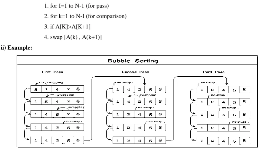
1. for I=1 to N-1 (for pass)

2. for k=1 to N-I (for comparison)

3. if A[K]>A[K+1]

4. swap [A(k) , A(k+1)]

ii) Example:

Fig 1: Working procedure of Bubble Sort

iii) Analysis:

Best Case: This time complexity can occur if the array is already sorted, and that means that no swap occurred

and only one iteration of n elements. O (n)

Worst case: The worst case is if the array is already sorted but in descending order. This means that in the first

iteration it would have to look at n elements, then after that it would look n - 1 elements (since the biggest

integer is at the end) and so on and so forth till 1 comparison occurs. Big Oh = n + n - 1 + n - 2 ... + 1 = (n*(n +

1))/2 = O ( n2₎

Average Case: O ( n2)

B) Selection Sort

It is among the most intuitive of all sorts. The basic rule of selection sort is to find out the smallest elements in

each pass and placed it in proper location. These steps are repeated until the list is sorted. This is the simplest

811 | P a g e

element is placed at the 0th position. The same procedure is repeated for 1th element and so on until the list is

sorted.

i) Algorithm:

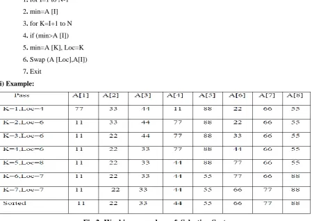
1. for I=1 to N-1

2. min=A [I]

3. for K=I+1 to N

4. if (min>A [I])

5. min=A [K], Loc=K

6. Swap (A [Loc],A[I])

7. Exit

ii) Example:

Fig 2: Working procedure of Selection Sort

iii) Analysis:Selecting the smallest element requires scanning all n elements, so this takes n − 1 comparisons

and then Swapping or interchanging it into the first position. Finding the next lowest element requires scanning

the remaining (n − 1) elements and so on, for (n − 1) + (n − 2) + ... + 2 + 1 = n (n − 1) / 2= O (n2)

Best Case: O (n2)

Average Case: O (n2)

Worst Case: O (n2)

C) Insertion Sort

It is an efficient algorithm for sorting a small number of elements. The insertion sort works just like its name

suggests, inserts each item into its proper place in the final list. Sorting a hand of playing card is one of the real

time examples of insertion sort. Insertion sort can take different amount of time to sort two input sequences of

the same sized epending upon how nearly they already sorted. It sort small array fast but big array very slow.

i) Algorithm

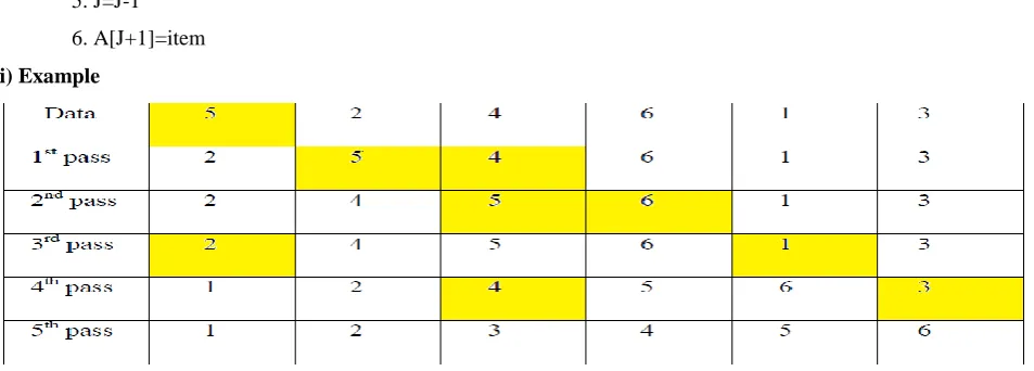
1. For I=2 to N

2. A[I]=item ,J=I-1

3. WHILE j>0 and item<A[J]

812 | P a g e

6. A[J+1]=item

ii) Example

Fig 3: Working procedure of Insertion Sort

iii) Analysis:

The implementation of insertion Sort shows that there are (n−1) passes to sort n . The iteration starts at position 1 and moves through position (n−1), as these are the elements that need to be inserted back into the sorted sub

lists. The maximum number of comparisons for an insertion sort is (n−1) .Total numbers of comparisons are: (n

− 1) + (n − 2) + ... + 2 + 1 = n (n − 1) / 2= O(n2)

Best Case: O (n2)

Average Case: O (n2)

Worst Case: O (n2)

D) Merge Sort

This sorting method is an example of the Divide-And-Conquer paradigm. This paradigm, divide-and-conquer,

breaks a problem into sub problems that are similar to the original problem, recursively solves the sub problems,

and finally combines the solutions to the sub problems to solve the original problem. Because

divide-and-conquer solves sub problems recursively, each sub problem must be smaller than the original problem.

i) Algorithm

void mergesort(int a[], int p, int r)

{

int q;

if(p < r)

{

q = floor( (p+r) / 2);

mergesort(a, p, q);

mergesort(a, q+1, r);

merge(a, p, q, r);

} }

void merge(int a[], int p, int q, int r)

{

int b[5]; //same size of a[]

813 | P a g e

while(i <= q && j <= r)

{

if(a[i] < a[j])

b[k++] = a[i++]; // same as b[k]=a[i]; k++; i++;

else

b[k++] = a[j++];

}

while(i <= q)

{

b[k++] = a[i++];

}

while(j <= r)

{

b[k++] = a[j++];

}

for(i=r; i >= p; i--)

{

a[i] = b[--k]; // copying back the sorted list to a[]

} }

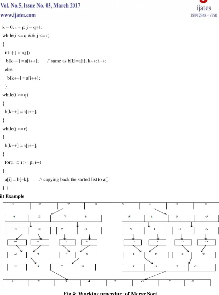
ii) Example

Fig 4: Working procedure of Merge Sort

iii) Analysis:In order to analyze the Merge Sort function, we need to consider the two distinct processes that

make up its implementation. First, the list is split into halves. We divide a list in half logn times where n is the

length of the list. The second process is the merge. Each item in the list will eventually be processed and placed

on the sorted list. So the merge operation which results in a list of size n requires n operations. The result of this

analysis is that logn splits, each of which costs n for a total of n (log n) operations.

Best Case: O (n log n)

814 | P a g e

E) Heap Sort

Heap Sort algorithm inserts all elements (from an unsorted array) into a heap then swap the first element

(maximum) with the last element(minimum) and reduce the heap size (array size) by one because last element is

already at its final location in the sorted array. Then we heapify the first element because swapping has broken

the max heap property. We continue this process until heap size remains one.

Here after swapping, it may not satisfy the heap property. So, we need to adjust the location of element to

maintain heap property. This process is called heapify. Here we Recursively fix the children until all of them

satisfy the heap property. some frequent terms use in this algorithm are,

Heap Property -> A data structure in which all nodes of the heap is either greater than equal to its children or

less than equal to its children.

Max-Heapify -> Process which satisfy max-heap property (A[parent[i]] >= A[i]). Here larger element is stored

at root.

Min-Heapify -> Process which satisfy min-heap property (A[parent[i]] <= A[i]). Here smaller element is stored

at root.

i) Algorithm

Since the maximum element of the array is stored at the root, A[1] we can exchange it with A[n]. If we now

“discard ” A[n], we observe that A[1...( n −1)] can easily be made into a max ‐heap. The children of the root

A[1] remain max ‐heaps, but the new root A[1] element may violate the max ‐heap property, so we need to

readjust the max ‐heap. That is to call MAX ‐ HEAPIFY(A, 1)

HEAPSORT(A)

1. BUILD‐MAX‐HEAP(A)

2. for i ← length[A] down to 2

3. do exchange A[1] A[i]

4. heap‐size[A] ← heap‐size[A] − 1

5. MAX ‐ HEAPIFY(A, 1)

815 | P a g e

Fig 5: Working procedure of Heap Sort

iii) Analysis

Worst Case: O (n log n)

Best Case: O (n log n)

Average Case: O (n log n)

F) Quick Sort:

Quick Sort is a Divide and Conquer algorithm. It picks an element as pivot and partitions the given array around

the picked pivot. There are many different versions of quick Sort that pick pivot in different ways.

1. Always pick first element as pivot.

2. Always pick last element as pivot (implemented below)

3. Pick a random element as pivot.

4. Pick median as pivot.

The key process in quick Sort is partition(). Target of partitions is, given an array and an element x of array as

pivot, put x at its correct position in sorted array and put all smaller elements (smaller than x) before x, and put

all greater elements (greater than x) after x. All this should be done in linear time.

i)Algorithm

Quicksort0 (A, p, r)

1: if p ≥ r then return

2: q = Partition(A, p, r)

3: Quicksort0 (A, p, q − 1)

816 | P a g e

Partition(A, p, r)

1: x = A[r]

2: i ← p − 1

3: for j ← p to r − 1 do 4: if A[j] ≤ x then

{

5: i ← i + 1

6: Exchange A[i] and A[j] }

7: Exchange A[i + 1] and A[r]

8: return i + 1

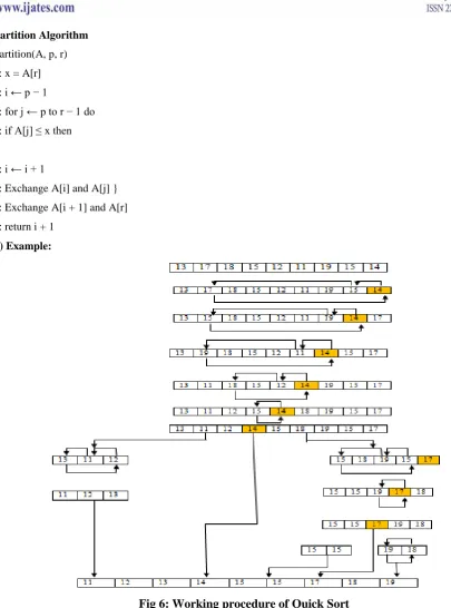
ii) Example:

Fig 6: Working procedure of Quick Sort

iii) Analysis

To analyze the Quick Sort algorithm of length n, if the partition always occurs in the middle of the list, there

will again be logn divisions. In order to find the split point, each of the n items needs to be checked against the

pivot value. The result is nlogn. In the worst case, the split points may not be in the middle and can be much

skewed to the left or the right, leaving a very uneven division. In this case, sorting a list of n items divides into

sorting a list of 0 items and a list of n−1 items. Then sorting a list of n−1, divides into a list of size 0 and list of

size n−2, and so on. The result is an O(n2) sort with all of the overhead that recursion requires.

817 | P a g e

Worst Case: O (n2)

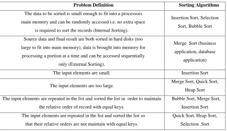
III. PROBLEM DEFINITION AND SORTING ALGORITHMS

All the sorting algorithms are problem specific. Each sorting algorithms work well on specific kind of

problems. In this table we described some problems and analyses that which sorting algorithm is more suitable

for that problem.

Problem Definition Sorting Algorithms

The data to be sorted is small enough to fit into a processors

main memory and can be randomly accessed i.e. no extra space

is required to sort the records (Internal Sorting).

Insertion Sort, Selection

Sort, Bubble Sort

Source data and final result are both sorted in hard disks (too

large to fit into main memory), data is brought into memory for

processing a portion at a time and can be accessed sequentially

only (External Sorting).

Merge Sort (business

application, database

application)

The input elements are small. Insertion Sort

The input elements are too large. Merge Sort, Quick Sort,

Heap Sort

The input elements are repeated in the list and sorted the list in order to maintain

the relative order of record with equal keys.

Bubble Sort, Merge Sort,

Insertion Sort

The input elements are repeated in the list and sorted the list so

that their relative orders are not maintain with equal keys.

Quick Sort, Heap Sort,

Selection Sort

Table 1: Problem Definition of various sorting algorithms

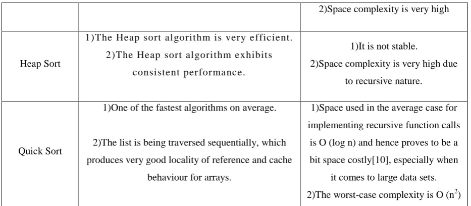
IV. ADVANTAGES AND DISADVANTAGES OF ALL SORTING ALGORITHMS

Sorting

Method Advantages Disadvantages

Bubble sort 1)Straightforward, simple and slow.

2)Stable. 1)Inefficient on large tables.

Selection Sort 1)Selection Sort is simple method.

2)No additional temporary storage is required.

1)Suitable for small list of elements.

2)General complexity is O (n2)

Insertion Sort

1)Insertion sort exhibits a good performance when

dealing with a small list.

2)The insertion sort is an in-place sorting algorithm

so the space requirement is minimal.

1)Insertion sort is useful only when

sorting a list of few elements.

Merge Sort

1)Time Complexity is O (n log n).

2)It can be used for both internal and external

sorting.

1)At least twice the memory

requirements of the other sorts

818 | P a g e

Heap Sort

1)The Heap sort algorithm is very efficient.

2)The Heap sort algorithm exhibits

consistent performance.

1)It is not stable.

2)Space complexity is very high due

to recursive nature.

Quick Sort

1)One of the fastest algorithms on average.

2)The list is being traversed sequentially, which

produces very good locality of reference and cache

behaviour for arrays.

1)Space used in the average case for

implementing recursive function calls

is O (log n) and hence proves to be a

bit space costly[10], especially when

it comes to large data sets.

2)The worst-case complexity is O (n2)

Table 2: Advantages and disadvantages of all sorting algorithms

V. COMPARATIVE ANALYSIS OF ALL SORTING ALGORITHMS

Every sorting algorithm has some advantages and disadvantages. In the following table we compared sorting

algorithms according to their complexity, memory used, stability, data type, method used by them like

exchange, insertion, selection, merge. In the following table, n represent the number of elements to be sorted.

The column Average worst case and Best case give the time complexity in each case. These all are comparison

sorting. To determine the good sorting algorithm, speed is the top consideration but other factor include

handling various data type, consistency of performance, length and complexity of code, and stability.

Sorting

Method

Average

Case

Worst

case Best case Method Stable

data

type complexity memory

Bubble

sort O(n

2

) O(n2) O(n) Exchange yes all very low NK+NP

Selection

Sort O(n

2_{) O(n}2_{) O(n}2_{) Insertion yes all very low NK+NP}

Insertion

Sort O(n

2

) O(n2) O(n2) Selection yes all very low NK+NP

Merge

Sort O(n log n) O(n log n) O(n log n) Merge yes all Medium

NK+2NP+

STACK

Heap Sort O(n log n) O(n log n) O(n log n) Selection no all Medium NK+NP

Quick Sort O(n log n) O(n2) O(n log n) Partition no all High NK+NP+S

TACK

Table 3: Comparative analysis of all sorting algorithms

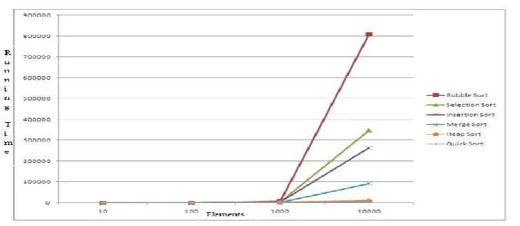
We implemented the all six sorting algorithms in C# for N=10. 100, 1000 and 10000, and calculated the run tine

819 | P a g e

N(Number of

elements) Bubble Sort Selection Sort Insertion Sort Merge Sort Heap Sort Quick Sort

10 204 253 227 539 513 305

100 299 298 246 614 689 324

1000 8397 3691 3281 3399 3414 615

10000 808927 347525 263501 91993 9315 3301

Table 4: RunTime

The graph constructed for the above table is given below in fig 7.

Fig 7: Graph representation of Run Time for all algorithms

IV. CONCLUSION

From the above analysis it can be said that, Bubble Sort, Insertion Sort and Selection Sort are fairly straight

forward, and easy to implement. Heap Sort, Merge Sort and Quick Sort are more complicated, but also much

faster for large lists. Quick sort is more often used as external sorting. Quick Sort is, on average, the fastest

algorithm but it needs enough memory. Bubble Sort algorithm is the slowest but needs no extra memory. On the

above comparison and the resultant analysis, it is clear to use Merge Sort, Heap Sort and Quick Sort for large

data sets whereas Bubble Sort, Selection Sort and Insertion Sort for small data sets.

REFERENCES

[1] Ahmed M. Aliyu and Dr. P. B. Zirra. 2013. A Comparative Analysis of Sorting Algorithms on Integer

and Character Arrays. The International Journal Of Engineering And Science (IJES).Volume.2. Issue.

7.Pages: 25-30.

[2] Astrachan, Owen. 2003 Bubble Sort: An Archaeological Algorithmic Analysis. SIGCSE, ACM.

Bender et al., (2006) Insertion Sort is O(n log n). Theory of Computing Systems 39 (3): 391.

[3] Sultanullah Jadoon, Salman Faiz Solehria, Mubashir Qayum, “Optimized Selection Sort Algorithm is

820 | P a g e

Computer Sciences IJECS-IJENS Vol: 11 No: 02.

[4] Tarundeep Singh Sodhi, Surmeet Kaur, Snehdeep Kaur, “Enhanced Insertion Sort Algorithm “,International

Journal of Computer Applications (0975–8887) Volume 64–No.21, February 2013.

[5 ] Deependra Kr. Dwivedi. 2011. Comparison Analysis of Best Sorting Algorithms. VSRD-IJCSIT, Vol.

1 (4), 2011, 261-267.

[6 ] Franceschini, Gianni, 2007. Sorting Stably, in Place, with O(n log n) Comparisons and O(n) Moves.

Theory of Computing Systems 40 (4): 327–353.

[7] J. S. Vitter. 2006. Algorithms and Data Structures for External Memory, Foundation and Trends in

Theoretical Computer Science, vol 2, no 4, pp 305–474. Lacey.Stephen and Box. Richard.1991. A Fast

Easy Sort. ACM. Volume 16 Issue 4:315

[8] Mishra.D.A, 2009. Selection of Best Sorting Algorithm for a Particular Problem. Computer Science

And Engineering Department Thapar University

[9] Oded Goldreich. 2008. Computational complexity: a conceptual perspective. Newsletter ACM

SIGACT News archive Volume 39 Issue 3, Pages 35-39.

[10] T. H. Cormen, et al.2001. Introduction to Algorithms. MIT Press, Cambridge, MA, 2nd edition.

AUTHORS

Ms. P.Reshma did her B.Tech in CSE from Vijaya Institute of Technology for Women, JNTU Kakinada and M.Tech in CSE from Dhanekula Institute of Engineering & Technology, JNTU Kakinada. Currently working as Assistant Professor in DVR & DHS MIC College of Technology.