Soft Lattices

(1)

University of Pennsylvania

ScholarlyCommons

Publicly Accessible Penn Dissertations

Summer 8-12-2011

Soft Lattices

Anton Souslov

University of Pennsylvania, [email protected]

Follow this and additional works at:

http://repository.upenn.edu/edissertations

Part of the

Condensed Matter Physics Commons

This paper is posted at ScholarlyCommons.http://repository.upenn.edu/edissertations/978 For more information, please [email protected].

Recommended Citation

Souslov, Anton, "Soft Lattices" (2011).Publicly Accessible Penn Dissertations. 978.

(2)

Soft Lattices

Abstract

We examine the elastic and vibrational properties of spring lattices, including the two-dimensional square and kagome and the three-dimensional cubic and pyrochlore lattices, which are at the verge of mechanical instability due to under-coordination. By using the extended Maxwell counting argument, we are able to count the number of soft phonon modes in these systems. These modes are stabilized by adding additional springs, bending energy terms or isotropic tension. By tuning the strength of these terms, we are able to continuously approach the mechanical instability to obtain scaling laws for the elastic moduli, as well as critical length and frequency scales. Further, these lattices can be deformed along their soft modes to obtain entire families of lattices with novel soft elastic properties. We find models of zero bulk modulus elasticity, leading to a negative Poisson ratio and a conformally invariant elasticity theory, whose implications we discuss. By following the mechanical instability, we obtain a full phase diagram of the isostatic point in these systems and encounter an unusual phase. In this phase, the ground state has a subextensive entropy, but at low temperatures the entropy of phonon fluctuations selects an ordered thermodynamic phase, through an elastic order-by-disorder effect. These properties are also compared to an elastic Ising antiferromagnet on a triangular lattice. We relate our models to physical systems, such as the jamming of granular media, semi-flexible

polymer gels and a quasi-two-dimensional colloidal experiment, and discuss their implications.

Degree Type

Dissertation

Degree Name

Doctor of Philosophy (PhD)

Graduate Group

Physics & Astronomy

First Advisor

Tom C. Lubensky

Keywords

jamming, isostaticity, square lattice, kagome lattice, pyrochlore lattice, elastic Ising model

Subject Categories

(3)

SOFT LATTICES

Anton Souslov

A DISSERTATION

in

Physics and Astronomy

Presented to the Faculties of the University of Pennsylvania

in

Partial Fulfillment of the Requirements for the

Degree of Doctor of Philosophy

2011

Supervisor of Dissertation

Signature

Tom C. Lubensky

Professor of Physics and Astronomy

Graduate Group Chairperson

Signature

A. T. Johnson, Professor of Physics and Astronomy

Dissertation Committee

Andrea J. Liu, Professor of Physics and Astronomy

Arjun G. Yodh, Professor of Physics and Astronomy

Douglas J. Durian, Professor of Physics and Astronomy

(4)

Soft Lattices

COPYRIGHT

2011

(5)

ABSTRACT

SOFT LATTICES

Anton Souslov

Tom C. Lubensky

We examine the elastic and vibrational properties of spring lattices, including the

two-dimensional square and kagome and the three-two-dimensional cubic and pyrochlore lattices,

which are at the verge of mechanical instability due to under-coordination. By using the

extended Maxwell counting argument, we are able to count the number of soft phonon

modes in these systems. These modes are stabilized by adding additional springs, bending

energy terms or isotropic tension. By tuning the strength of these terms, we are able to

continuously approach the mechanical instability to obtain scaling laws for the elastic

mod-uli, as well as critical length and frequency scales. Further, these lattices can be deformed

along their soft modes to obtain entire families of lattices with novel soft elastic

proper-ties. We find models of zero bulk modulus elasticity, leading to a negative Poisson ratio

and a conformally invariant elasticity theory, whose implications we discuss. By following

the mechanical instability, we obtain a full phase diagram of the isostatic point in these

systems and encounter an unusual phase. In this phase, the ground state has a

subexten-sive entropy, but at low temperatures the entropy of phonon fluctuations selects an ordered

thermodynamic phase, through an elastic order-by-disorder effect. These properties are also

compared to an elastic Ising antiferromagnet on a triangular lattice. We relate our models

to physical systems, such as the jamming of granular media, semi-flexible polymer gels and

(6)

List of Tables

2.1 Comparison of frequencies, lengths, and elastic moduli of square, kagome,

deformed kagome and pyrochlore lattices to the marginally-jammed (MJ)

(11)

List of Figures

1.1 A simple example of redundant bonds, states of self stress and the extension

of Maxwell’s counting argument . . . 14

2.1 The honeycomb and the small rhombitrihexagonal sub-isostatic lattices . . 26

2.2 The phonon dispersion relation of the honeycomb lattice in the 1stBZ for the

lowest mode, the KΓMK cut and the density of states . . . 27

2.3 Plots of the square lattice, showing the isostatic lattice and the lattice with

NNN bonds . . . 29

2.4 Phonon dispersion relation of the square lattice, with the 1st_{BZ of the lowest}

mode and the RΓMR cut. . . 30

2.5 3D plots for the dispersion of the square lattice . . . 30

2.6 Examples of soft modes of the square lattice . . . 31

2.7 Plots of the kagome lattice, showing the isostatic lattice and the lattice with

NNN bonds . . . 38

2.8 Reduced density of states as a function of frequency for the square and

kagome lattices . . . 39

2.9 The phonon dispersion relation of the kagome lattice along the KΓMK cut . 39

2.10 The phonon dispersion relation of the kagome lattice in the 1st_{BZ for the}

lowest mode . . . 40

2.11 Dispersion of the quasi-isostatic mode of the kagome lattice, showing the

effects of pressure and the validity of the perturbative expansion . . . 40

3.1 The brick lattice and the inverted honeycomb lattice as part of a family of

deformed honeycomb lattices . . . 52

3.2 Various deformations of the square lattice . . . 53

(12)

3.4 The phonon dispersion relation of the pmg:ptM deformed square lattice . . 54

3.5 The phonon dispersion relation of the p1 deformed square lattice . . . 55

3.6 Various soft deformations of the kagome lattice . . . 57

3.7 The phonon dispersion relation of the p31m:ptΓ deformed kagome lattice . 57

3.8 Plots of the Poisson ratio and the bulk and shear moduli of the p31m:ptΓ

deformed kagome lattice . . . 58

3.9 Phonon dispersion relation of the pgg:ptM deformed kagome lattice . . . 62

3.10 Phonon dispersion relation of the p6:pt3xM deformed kagome lattice . . . . 63

4.1 Plots of the cubic lattice and its density of states . . . 66

4.2 3D plots of the pyrochlore lattice and its unit cell . . . 68

4.3 The soft phonon modes in the 1stBZ of the pyrochlore lattice and the phonon

dispersion relation along the ΓXWLΓKX’ cut . . . 72

5.1 Plots of the ground state of the square lattice with negative NNN spring

constants k′ _{. . . .} ₈₀

5.2 The free energy difference between the straight and bent stripe square lattice

ground state configurations at low temperature . . . 82

5.3 Numerical phase diagram of the square lattice with negative NNN spring

constantk′ . . . 83

5.4 Ground state plaquettes of the antiferromagnetic elastic Ising model on a

triangular lattice . . . 85

5.5 A sample ground state configuration of the antiferromagnetic elastic Ising

model on a triangular lattice . . . 86

5.6 Phonon dispersion relations for the triangular lattice . . . 91

5.7 Dispersion relations for the phonon modes of the elastic Ising model straight

and bent stripe ground states with α= 55◦ _{. . . .} ₉₂

(13)

and bent stripe ground states with α= 12.5◦ . . . 94

5.10 The free energies and the difference in free energies for the straight and bent

stripe configurations of the elastic Ising model . . . 97

5.11 Examples of ground states of the elastic Ising model with large unit cells . . 98

5.12 Rescaled free energy versus the proportion of bent nearest neighbor

(14)

Chapter 1 Motivation and Background

1.1 Introduction

This thesis explores certain aspects of soft elasticity arising from the approach to

iso-staticity. Such softness arises from under-coordination, i.e. too few inter-particle

interac-tions to stabilize all of the individual degrees of freedom in the system. Due to the abstract

nature of the theoretical framework, it is widely applicable to soft materials ranging from

jamming of granular media to elasticity of semi-flexible polymer gels. In addition, by

in-corporating Ising degrees of freedom in our system, we are able to apply these techniques

to an experimental system of a quasi-two-dimensional colloid.

By starting with concrete microscopic models, we are able to present rigorous analytic

arguments for their elastic behavior. These models can be regarded as examples in a wider

class of soft systems, and their examples illustrate certain universal aspects of isostaticity.

Further, by taking a survey of various lattice geometries, we are able to make generalizations

about the non-universal, configuration-dependent aspects of elasticity in such systems.

The framework of elasticity serves as a well developed launch pad, and its power has

been applied to a wide array of systems exhibiting interesting aspects of softness. Rubber

elasticity, more recently extended to liquid crystal elastomers is a striking example.

1.2 Jamming

It has been observed that certain disordered systems undergo a dramatic change in

behavior over a small parameter range, particularly in their mechanical properties. [32,

(15)

temperatures, lower density and higher driving forces, we observe a behavior similar to

that of a perfect fluid, with a dynamic response to deformations characterized by a certain

macroscopic flow field. However, as the system is driven less, cooled or compressed, we note

a rapid increase in the response to the deformation. Thus the system starts to acquire the

behavioral properties of a solid, developing a shear modulus, without establishing any sort

of positional order between its constituent particles.

These phenomena can be described under the conceptual framework of jamming, which

unites similar behavior in certain parameter ranges of materials as varied as granular

sys-tems, atomic and molecular glasses, gels, colloids, foams, and emulsions. It also provides

an example of the physics associated with isostaticity. These systems can be studies both

experimentally, by preparing them under the proper conditions, and theoretically. The

lat-ter approach has been used to study various examples through numerical simulations. In

order to simulate large systems efficiently certain simplifications must be made, and many

simulations use either hard sphere, repulsive soft spheres, or Lennard-Jones type models.

There has been some work done to try to understand the fundamental nature of the

behav-ior of these systems through heuristic theoretical arguments. In contrast, this work explores

lattice models that can be solved exactly to develop rigorous arguments for the nature of

elastic response in nearly isostatic systems.

1.2.1 Jamming of Granular Media

Granular matter falls into a particular class of systems that have neither large thermal

fluctuations nor any notable driving forces, in which case the density becomes the only

varied control parameter. Numerical simulation indicate a sharp transition from a rigid,

shear-supporting state in such cases, e.g. for repulsive spheres, without any indication of

order. [11, 41, 42] It is known that in two or three dimensions, the densest sphere packings

are ordered structures. In two dimensions, mono-disperse disks easily crystallize into a

hexagonal lattice, since it both locally and globally maximizes the free volume of the disks.

As a result, simulations only produce random glassy states in hard-disk systems with two

(16)

random static jammed state seems accessible, even for mono-disperse spheres. [11, 41, 42]

The designation Point J is used to identify the static athermal transition in sphere

packings. The difficulty in characterizing it comes from the interplay of the mechanical

stability, disorder, and pressure in these systems. An important question arises as to the

universality of certain numerical observations, for example whether they are restricted to

the theoretical spheres or whether they might be general enough to apply to an experimental

system.

If point J is indeed a phase transition, we ask how a system behaves near that point. Can

we find scaling? Are there any divergent lengths? Do any quantities exhibit discontinuous

jumps? Based on numerical simulations and some theoretical arguments, positive answers

have been given to all of these questions. If we characterize the transition by a densityφc,

it would be useful to find scaling in terms of ∆φ=φ₋φc. [11, 41, 42]

1.3 Isostaticity

To motivate further analysis, the concept of isostaticity must be introduced, followed

by a brief overview of the arguments based on that concept.

1.3.1 Maxwell Counting Argument

James C. Maxwell[35] asked what generic conditions are necessary to mechanically

sta-bilize a system of N particles. The answer turns out to be a relatively simple counting

argument. If a system of N non-interacting particles lives in d dimensions, it has dN

de-grees of freedom. Thus, if interactions are added the system will be marginally stable if

there are dN linearly independent equations of mechanical constraint on the system. More

constraints result in a more stable system. However, if the number of constraints if below

dN, the system will have certain deformations that do not cost any energy. Such

defor-mations are soft and represent the failure modes of an unstable system. This result has

been applied to many systems [1, 68], including network glasses[43, 60], rigidity percolation

[27, 12], β-cristobalite [57], granular media [14, 61], protein folding [44], and elasticity in

(17)

If a particle interacts with a neighbor via a central force, then there will be a constraint

for that pair, taking away one degree of freedom for the two particles. The average number

of neighbors with which each particle interacts is called thecoordination number z. Such a

system has 1₂zN constraints. Thus, when dN = 1₂zN the system will be marginally stable,

andzc = 2dwill signify the onset of rigidity. A system with the critical coordination number

is called isostatic, and the distance away from this point is ∆z=z₋zc.

Disorder makes a granular medium isotropic and homogeneous and assures that below

isostaticity the system of equations of constraint is linearly independent, since the bonds

are randomly oriented. Below point J, when the system is fluid-like, z= 0, as the particles

do not touch, while at point J, z jumps to zc. Above point J, in the jammed state, it has

been determined through numerical work that ∆z_∼(∆φ)1/2[11, 42]. For simplicity, we can

characterize the scalings in terms of ∆zin the jammed state, based on numerical simulations.

The elastic constants of the system scale, with the shear modulus µ_∼∆z, while the bulk

modulus remains constant,B _∼(∆z)0 [11, 42]. There are other critical quantities that can

be extracted from these simulations, including divergent critical length scales ℓ∗

1 ∼(∆z)−1

and ℓ∗

2 ∼(∆z)−1/2 [53, 72] and a vanishing critical frequency ω∗ ∼(∆z)1. [53, 15] These

are obtained by looking at the propagation of elastic waves and the elastic response.[71, 70]

1.3.2 The Cutting Argument

We look at a large system with a small ∆z, i.e. slightly above isostaticity. We can

cut out a regularly shaped region with N particles by cutting a certain number of bonds.

Since the number of bonds cut is proportional to the hypersurface enclosing the region,

whose area scales as N(d−1)/d, the coordination number of the cut out region decreases

by N−1/d_{. A small enough region will thus be sub-isostatic, while a large enough region}

will be hyper-isostatic. In between, there must be a characteristic system size such that

the cut out region is exactly at isostaticity. This length scale ℓ∗ _{associated with the cut}

scales as ℓ∗ _∼ V1/d _∼ N1/d _∼ (∆z)−1.[68] This argument can be further extended to

include a frequency scale ω∗. Since ℓ∗ can be seen as the wavelength of a certain elastic

(18)

that vanishes at isostaticity, ω∗_∼ _ℓc∗ ∼(∆z)1.[68]

Using an extension of this argument, the scaling of elastic moduli for the response to

shear µ _∼ ∆z and bulk B _∼ (∆z)0 deformations can be derived.[68] This is done by

substituting ℓ∗ into a variational argument, which requires further assumptions about the

geometry of particle configurations.

1.3.3 The Geometry of Isostatic Systems

Since these scalings are expressed in terms of the coordination number ∆z, which serves

as an indicator of mechanical stability, one might wonder whether the scaling laws are just

the result of the system being at the verge of an instability. In other words, whether the

topology of the spring network solely determines its elastic properties. This does not take

into account any information about particle configurations, including disorder. In order to

answer this question, we must apply the counting argument to a wide range of systems,

juxtaposing their scaling near isostaticity. The isostatic lattice models we consider provide

a rigorous means to do so.

1.4 Semi-Flexible Polymer Gels

Another relevant aspect of soft elasticity comes from the study of semi-flexible polymer

gels. At the microscopic level, these systems are a network of almost straight rods, which

are randomly cross-linked to give the system a response to shear.[66, 26, 24]

Thus, a counting argument can be applied to this system, provided that all constraints

are properly included. Cross-links essentially play the role of point particles, while the

polymers connecting them act as interactions. The coordination number can then be seen

as fixed at z= 4, independent of dimensionality. While central force repulsion comes from

the resistance of polymers to compression, there are other constraints on the system. Due

to the long persistence length, the polymers do not bend easily at the cross-links, especially

as their density is increased, which gives two more constraints for every cross-link in the

(19)

cross-linking procedure, essentially just adding more equations of constraint to the system.

1.5 Linear Elasticity

Anelastic deformation is a map from the undeformed reference state, with a continuum

of points x, into a target space marked by

R(x) =x+u(x), (1.1)

whereu(x) is the displacement vector. If the deformation isuniform,

R(x) = Λx=x+ηx (1.2)

where the deformation tensor Λ is a spacially independent matrix and η= Λ₋I.

More generally, a spacially varying displacement can be described by a strain,

uij(x) =

1

2(∂iuj+∂jui+∂kui∂kuj). (1.3)

The elastic free energy of uniform deformations to lowest order must then have the form

F = 1

2

Z

ddxCijkluijukl, (1.4)

whereCijkl is the elastic constant tensor anddis the dimensionality of the system.[31] Note

that to lowest order, only the first two terms of the strain tensor are necessary,

uij(x) =

1

2(∂iuj+∂jui)≡ 1

2(ηij+ηji). (1.5)

This expression can also be transformed to Fourier space, and the free energy written

as

F = 1

2

Z

d2q

(2π)2ui(−q)Dij(q)uj(q). (1.6)

(20)

Note that the equations for stability under an applied external stress σij are simply

δF

δu =σij, or

Cijkl∂j∂kul=σij. (1.7)

1.5.1 Elastic Moduli

For a stable isotropic system,

Cijkl =λδijδkl+µ(δikδjl+δilδjk) (1.8)

where the two elastic moduliλ and µ, called the Lam´e coefficients, correspond to the two

different rotationally invariant rank four tensors that can be constructed from the Kronecker

δ.[31] In that case, elastic free energy can be written as

Fiso = 1

2

Z

ddx λu2_ii+ 2µu2_ij

= 1

2

Z

ddx

Bu2_ii+ 2µ(ujk−

1

dδjkuii)

2

(1.9)

where theshear modulusµdetermines the response to shear distortions and thebulk modulus

B =λ+2_dµdetermines the response to isotropic compression. In two dimensions, this takes

an even more compact form,

F2Diso=

1 2

Z

d2x B(uxx+uyy)2+µ(uxx−uyy)2+ 4u2xy

(1.10)

For anisotropic systems, the structure of Cijkl reflects the point symmetry group of the

underlying solid. In two dimensions, lattices with 3- or 6-fold point symmetry still have

only two elastic moduli, and a linear elasticity indistinguishable from that of an isotropic

solid. A lattice with square symmetry, however, has three different elastic moduli instead,

Fsq= 1

2

Z

d2x C11(u2xx+u2yy) + 2C12uxxuyy+ 4C44u2xy

(21)

For the three dimensional cubic lattice, the expression is very similar,

Fc = 1

2

Z

d3xC11(u2_xx+u2_yy+u2_zz) + 2C12(uxxuyy+uxxuzz+uyyuzz) + 4C44(u2xy+u2xz+u2yz)

(1.12)

The rhombohedral lattices have an even lower symmetry group, with six independent

coefficients.

Frhomb= 1

2

Z

d3x

Bxy(uxx+uyy)2+µxy

(uxx−uyy)2+ 4u2xy

+C33u2zz

+C55(u2xz+uyz2 ) +C13uzz(uxx+uyy) +C15[(uxx−uyy)uxz−2uxzuyz]

(1.13)

whereBxy and µxy denote, respectively, the moduli for bulk and shear deformations in the

xy-plane.[31]

1.5.2 Negative Poisson Ratio

Another useful parameter for describing elastic properties of solids is thePoisson ratio.

This denotes the ratio of the compression of the perpendicular cross-section due to a uniaxial

tension. For an isotropic material this is a scalar,

σ= dB−2µ

d(d₋1)B+ 2µ (1.14)

where the relevant cases areσ = _λ₊₂λ_µ in 2D orσ = ₂₍_λλ₊_µ₎ in 3D. In general,₋1< σ < _d₋1₁

though for most common materials it is positive. In particular, perfectly incompressible

three-dimensional materials have σ= 1₂ and rubbers are close to this limit.

On the other hand, certain materials have negative Poisson ratios, σ < 0. These can

also be called auxetics or anti-rubbers. Materials with zero bulk modulus, B = 0, provide

an extreme case of a negative Poisson ratio,σ =₋1.

A common material with a nearly zero Poisson ratio is cork, where the elastic properties

are used to insert the seal into the bottle and prevent it from unsealing too easily. However,

(22)

prevalent, where the geometry of the components is designed to provide auxetic behavior.

[29]

A common model of an auxetic material can be found by using the honeycomb topology.

By proper deformations, an auxetic lattice, called the inverted honeycomb lattice, can be

created. It has low symmetry and a particular axis with a large negative Poisson ratio.

[18, 29, 17, 7] However, in order for this model to be elastically stable, rigid rods must

replace springs in some of the bonds. Other models have also been considered, but tension

or rigid rods are most often used to guarantee the stability of such an elastic system.[45, 2]

Recently, it has been noted that the elasticity of a deformed kagome lattice also has auxetic

behavior. [13, 19]

1.5.3 Zero Bulk Modulus: Topological Properties

The elastic free energy for an isotropic material with a zero bulk modulus has the form

FB=0 =µ

Z

ddx(ujk−

1

dδjkuii)

2 _(1.15)

An interesting observation is that such a theory is invariant under conformal

transfor-mations. [47, 39] To see this, we express the elastic free energy in a more geometric form,

in terms of the metric tensor defining the deformation in Eq. 1.1. The metric tensor g of

the target space is defined as

gij =

∂R(x)

∂xi ·

∂R(x)

∂xj

(1.16)

For instance, the metric tensor of a undistorted systems is g◦ =I.

Conformal transformations correspond to deformations satisfying

g(x) =f(x)I (1.17)

withf(x) being an arbitrary smooth function of x.

(23)

unchanged. Rewriting the elastic free energy in terms of the metric tensor

F = 1

2

Z

ddx[B(trg)2+µtr(g−1

dItrg)

2_]_, _(1.18)

we see that for systems with B >0 and µ >0, the only soft deformations are of the form

g =I, corresponding to rigid body motions of translations and rotations. However, when

B = 0, the elastic energy in Eq. 1.18 depends only on the traceless part of g. Thus, it we

can see that an elastic deformation will cost no energy if and only if Eq. 1.17 is satisfied. In

other words, Eq. 1.15 is conformally invariant and therefore the soft deformations for zero

bulk modulus isotropic elasticity are exactly the conformal transformations of space.[47, 39]

If we consider the stability of such a model without external stress, Eq. 1.7 reduces

to Laplace’s equation, _∇2_u _{= 0. Thus, we see that the solutions are determined by the}

boundary conditions, and many displacements exist that do not change the elastic free

energy_F, their “number” somehow dependent on the length of the boundary.

Conformal symmetry makes such an elastic model part of a much larger interesting

class of topological states of matter. Thus, analogy can be drawn between such a model

and quantum topological states such as the integer and fractional quantum Hall effects, the

quantum spin Hall effect and the resonating valence bond states in spin liquids.

1.5.4 Cosserat Elasticity

While classical elasticity describes the behavior of uniform solids, certain materials are

not well described by the assumption of affine response. Instead, they experience

microro-tations under certain forms of stress, which are not taken into account in Eq. 1.4. These

microrotations must couple to the strain to form a scalar free energy density. Since a

rotational degree of freedom, φ is a pseudoscalar, it must thus couple to _{∇ ×}u, or the

anti-symmetric part of η. A fundamental assumption of Cosserat elasticity is that due to

(24)

then have the lowest order form

F =

Z

dx

Bu2_ii+µu˜2_ij+κ(φ₋1

2∇ ×u) 2₊_ξ₍

∇φ)2

. (1.19)

Note that ifκ is large,φ will not be easily excited and can be integrated out of the elastic

free energy. In contrast, if κ= 0, φwill be a soft mode involving microrotations. Another

interesting case comes when B = 0. Then, the conformal invariance of the elastic free

energy extends to Cosserat elasticity as well, since the new terms are not affected under

conformal transformations.[39]

1.6 Structural Phase Transitions and Beyond

If we are considering an elastic free energy at the verge of an instability, it can be

proper to add a higher order stabilizing term consistent with the symmetry of the lattice.

For example, we add a curvature term to the square lattice elasticity,

F = 1

2

Z

d2x[C11(uxx2 +u2yy) + 2C11uxxuyy+ 4C44u2xy+K(∇2u)2], (1.20)

This harmonic energy can transformed to Fourier space

F = 1

2

Z

d2q

(2π)2ui(−q)Dij(q)uj(q), (1.21)

where

Dxx = C11qx2+C44q2y+Kq4

Dyy = C11qy2+C44qx2+Kq4

Dxy = Cyx = (C12+C44)qxqy. (1.22)

AsC44∼ |T−Tc| →0 asT →Tc, there is an incipient instability toward the simple shear

distortions shown in Fig.3.2(a), and the development of long-range correlations. Comparison

(25)

length

ξ =

r

K C44 ∼ |

T ₋T_c|−1/2. (1.23)

To stabilize the system whenC44<0 we add to F a quartic term inuxy, 1₄gu4xy. Then for

C44<0,

uxy =± p

−C44/g∼ |T−Tc|1/2. (1.24)

X-ray or neutron scattering experiments measure the displacement correlation function

Sij(q) = kBT χij(q) ≡kBT Cij−1(q) and thus the vanishing of C44 and the diverging

corre-lating lengthξ as can be seen from

Sxx(0, qy) =

kBT

C44q2y+Kq4y

= kBT

C44 1 1 +q2

yξ2

. (1.25)

The frequencies of dynamical modes are determined by ρω2δij = Cij(q), where ρ is the

mass density. Thus the shear sound velocity,pC44/ρ, vanishes as |T −Tc|1/2 asC44→0.

For a lattice with hexagonal symmetry, we again add a curvature termK(_∇2_u₎2 _{to the}

elastic free energy in Eq. 1.9. When µ _→ 0, there is an instability to a sheared state in

which the symmetric-traceless strain, ˜uij =uij − 1₂δijukk =S(ninj −1₂δij) where ni is an

arbitrary unit vector, develops a nonzero value. To stabilize the energy when µ becomes

negative, we add a term 1₄g(˜uij)4 (there is no third order term in 2d), and as in the case of

the square lattice, we can identify a diverging length scaleξ, a vanishing order parameter,

and a vanishing sound velocity:

ξ =

s

K

µ ∼ |T−Tc|−

1/2 _(1.26)

S = p₋µ/g_{∼ |}T ₋T_c|1/2 (1.27)

ct = p

µ/ρ_{∼∼ |}T ₋T_c|1/2 (1.28)

1.7 Beyond Maxwell Counting

Maxwell counting proves remarkably accurate at predicting the critical coordination

(26)

systems, since the count is global. However, in certain cases stability can be highly

depen-dent on the local configurations.

1.7.1 Laman’s Theorem and the Pebble Game

A local version of Maxwell counting for generic systems in mechanical equilibrium can

be developed based solely on the topology (i.e. connectivity) of the contact network. [30]

The pebble game implements this counting on a network, locating floppy, isostatic and

over-constrained regions.[27] While studying this generic rigidity percolation has provided

insight for fundamental understanding of statistical mechanics, it has also been successfully

applied to account for the mechanical properties of large biomolecules, which cannot be

easily simulated at the atomic scale. [28]

1.7.2 The Equilibrium and Compatibility Matrices

A more general extension of the counting argument needs to account for the precise

particle configurations and interactions. This involves relating the dN-dimensional vector

of particle displacements d to theNB-dimensional vector of spring stretchesethrough the

compatibility matrix C,C_·d=e. Equivalently, we can relate the tensions in the springst

to the forces on each particlef, through theequilibrium matrix H_·t=f. These are in fact

related,C_≡HT.[5] Further, using Hooke’s law which relates the stretches to the tensions,

t =K_·e, where K are the generalized spring constants for the bonds, we get a force law

f =H_·K_·C_·d or, provided these is a single spring constant,K=kI,

f =kH_·HT_·d. (1.29)

1.7.3 Singular Cases and States of Self Stress

While the Maxwell count is essentially a dimensionality argument for the matricesHand

C, interesting results arise when these matrices have a non-trivial nullspace. The nullspace

of H consists of states of self stress, that is a single configuration where stresses can be

(27)

Figure 1.1: (Color Online) (a) When b > 3a, the generic Maxwell counting argument applies. These four particles have eight degrees of freedom and four constraints in the form of bonds, leaving 3 rigid body motions and one soft mode. (b) In the singular case,

b = 3a, there is instead one state of self stress and two soft modes, corresponding to the displacements of two of the particles perpendicular to the bonds. Note that while the mode in (a) is soft to all orders, allowing for finite deformations, the soft modes in (b) are infinitesimal, and no soft finite deformation is present.

deformations. For an isostatic system, since C_≡HT, each state of self stress results in an

extra mechanism. In general, the number of soft modes isdN ₋T ₋NB+S, where T are

the d translations and d(d₋1)/2 rotations, NB is the total number of bonds (in general,

constraints) and S is the number of states of self stress. Fig.1.1 shows a basic example of

this extension of Maxwell counting.

1.8 Spring Lattice Models

While linear elasticity allows us to examine the long wavelength response of soft solids,

these models need to be expanded to study the frequency dependent response. A

ball-and-spring lattice provides a natural microscopic model for an elastic solid. We take a periodic

tiling of Euclidean space, place particles of mass m = 1 at the nodes of the tiling and

connect certain pairs of with springs of potential energyVij. This can be seen in Figs. (2.1

2.3, 2.7, 3.1, 3.2, 3.6, 4.1(a), 4.2) for a variety of lattices.

1.8.1 Dynamical Matrix from a Free Energy

The potential energy of the spring between particles iand j will be

Vij(|ri−rj|) =

1

2kij(|ri−rj| −aij)

2 _(1.30)

where kij is the bond’s spring constant, ri,j are the positions andaij is the rest length of

(28)

This model can be solved to lowest order in the particle displacements ui from the

equilibrium positionr◦_i, where ri=r◦i +ui. In order to do so, Eq. 1.30 must be expanded

to lowest order inui. Since the lattice is stable,∂V /∂ui=0for allui and we must expand

to second order. First, we consider the case of unstressed springs, [3]

Vij =

1

2kij(|r◦i −rj◦+ui−uj| −aij)

2 _≈ 1

2kij

_r◦ i −r◦j

aij ·

(ui−uj) 2

. (1.31)

The total potential energy is then the sum over every spring,

Vtotal=

1 2

X

hi,ji

kij _r◦

i −r◦j

aij ·

(ui−uj) 2

. (1.32)

Such notation is reminiscent of a bilinear form Di,j, where ui is regarded as a single

vector of length dN, where N is the number of particles in the lattice,

V = 1 2

X

hi,ji

ui·Di,j·uj (1.33)

Note that the force law derived using the compatibility and equilibrium matrices in Eq.(1.29)

provides a completely equivalent description, with Di,j ≡H·K·C≡ kH·HT where the

later equivalence assumes a single spring constantkfor all of the lattice springs.

This expression can be Fourier transformed, yielding a quadratic Hamiltonian [3]

H= 1

2

X

hi,ji

u†(q)_·D(q)_·u(q) (1.34)

which can be decomposed into a sum over unit cells and the sum within a single unit

cell. For an infinite periodic lattice, the sum can be transformed into an integral over a

continuous periodic space ofq. The expression forD(q) within a unit cell of the reciprocal

space, called the first Brillouin zone (1stBZ) provides the modes of the entire lattice. This

allows us to consideru(q) as a vector in dNc-dimensional space, whereNc is the number of

(29)

1.8.2 Phonon Modes

DiagonalizingD(q) gives the quadratic modes of the system as the eigenvectors and the

dispersion relation for the square of the mode frequencies ω2(q) as the eigenvalues, since

∂_H ∂u† =−

∂2u ∂t2 =ω

2₍_q₎_u _(1.35)

from the wave equation, wherem= 1. Note that sinceDi,j is symmetric underi↔j,D(q)

is unitary and the eigenvalues are real, as physically necessary. Further, the stability of the

lattice guarantees thatD(q) is nonnegative-definite and thusω(q) is real.

1.8.3 Linear Elasticity of Spring Lattices

The dynamical matrix gives more information than a theory of linear elasticity, since

it considers short wavelength distortions. However, by expanding the dynamical matrix to

lowest order inq, we get

Dik(q)≈qjCijklql+O(q3) (1.36)

We can thus always write down

H ≈ 1

2

Z

ddq C_L2q2_|u_L|2+

d−1

X

i=1

(C_Ti)2q2_|ui_T_|2

!

(1.37)

where CL is the sound velocity for the longitudinal phonon mode, while {C_Ti}d_i₌₁−1 are the

sound velocities for the transverse phonons. Note that for two-dimensional lattices with two

elastic moduli, CL = p

(λ+ 2µ)/ρ and CT = p

µ/ρ, where ρ is the lattice mass density.

For anisotropic system, the sound velocities are direction dependent.

While disordered solids do not have well-defined wavenumbers for their phonon modes,

they do have a phonon spectrum resulting in a Density Of States (DOS). This can be

(30)

expressed as an integral over the 1stBZby substituting the dispersion relation ωi(q),

d(ω) = X

n∈modes

δ(ω₋ωn) = X

i

2_|ω_|

Z

1st

BZ

dq

(2π)2δ(ω

2₋_ω2

i(q)) (1.38)

[3] The DOS can also be calculated for each individual modeωi(q).

For isotropic stable two-dimensional solids, near the origin q = 0, the DOS receives

contributions from the longitudinal and transverse phonons, each mode contributingdi(ω) =

ω

2πC2. In general, for a stable lattice, the DOS is expected to scale as d(ω) ∼ ωd−1 near ω= 0 due to the Debye argument. In a lattice with an infinite number of soft deformations,

a singularity will appear at d(ω= 0) to reflect these states.

An interesting observation arises from comparing the soft uniform deformations of a

lattice, defined by

Cijklηkl◦ = 0 (1.39)

to long wavelength soft phonons, which must satisfyDik(0)uk=0 to all orders inq.

To lowest order, this means

niq◦jCijklqk◦nl= 0 (1.40)

a condition distinct from that of Eq. 1.39. Thus, we will encounter lattices which have soft

uniform deformations without soft phonon modes and vice versa.

1.9 A Survey of Lattices Considered

These several techniques – global Maxwell counting, local force balance, the equilibrium

and compatibility matrices, the theory of linear elasticity, and the phonon spectrum – allow

us to fully characterize the soft behavior of nearly isostatic lattices.[54]

1.9.1 Square and Cubic Topologies

Perhaps the simplest class of isostatic lattices revolves around the two-dimensional

square and the three-dimensional cubic lattices. (Figs. 2.3, 4.1(a))

(31)

consequence, their spectrum will only have thedacoustic phonons. Taking into account the

states of self stress, there must be some soft phonons modes. Near the origin,q=0, these

are the transverse acoustic phonons, corresponding to the states of soft uniform shear. The

soft phonons at shorter qcorrespond to local shear.

Thus, the square lattice has a soft affine deformation, differentiating it from granular

packings. It can be deformed into various other lattice geometries without changing its

bond lengths. We also consider a lattice with less symmetry constructed by using the

square lattice topology and arbitrary spring lengths.

1.9.2 Kagome and Pyrochlore Topologies

By contrast, the kagome (pyrochlore) lattice has triangles (tetrahedra). (Figs. 2.7, 4.2)

Since these simplexes are defined by the length of their sides, they are incompatible with

affine soft deformations. Instead, they have 3(4) particles per units cell, with soft optical

phonons arising from the states of self stress.

These soft modes correspond to local microrotations of the triangles (tetrahedra). Near

isostaticity these can couple with the acoustic phonons, resulting in a low-energy theory

reminiscent of Cosserat elasticity.

When the lattice is deformed along these modes, the soft phonons couple to volume

change, resulting in a lattice with (a) soft uniform deformation(s). [13] In highly symmetric

cases of the deformed kagome lattice, this results in an isotropic linear elasticity with a zero

bulk modulus. However, the low-symmetry deformations of lattices with the kagome and

pyrochlore topologies have low-symmetry soft uniform deformations.

1.10 Stabilizing Terms

1.10.1 Next-Nearest Neighbors and the Approach to Isostaticity

Note that for all of the lattices we are considering, adding the NNN springs will

sta-bilize them into a solid, providing a finite energy for all of the possible relative particle

(32)

direct calculations.

Hyper-isostatic lattices are stable with NN springs, by definition. However, for lattices

at or below isostaticity, soft deformations are stabilized by adding NNN springs. Thus,

we take all NN springs to have the spring constant k, while NNN springs have the spring

constant k′. Importantly, as k′/k _→ 0, we recover back the soft modes, so that this limit

allows us to continuously approach the isostatic transition. Note that for generic springs, a

hyper-isostatic system will be under a state of self-stress. However, instead we pick all the

spring rest lengths so that the springs are at rest without external stresses.

There are several other means of approaching the isostatic transition by introducing

additional terms in the Hamiltonian, thus adding more constraints to the total degrees of

freedom of the system.

1.10.2 States of Stress

One means of stabilizing the soft modes of an isostatic system is to put it under uniform

tension, i.e. a negative pressure. For a stable isotropic solid, to lowest order the pressure

simply modifies the elastic moduli as λ _→ λ+p and µ _→ µ ₋p. Extending this to

lattice models, we must linearize the spring potential in Eq. 1.30 around some spring

length_|r◦_j₋r◦_i_{| ≡}R_ijo ₆=aij. While the Hamiltonian of unstressed springs in Eq. 1.31 was

proportional toV′′= ∂2_∂RV(oR2o) =kij, here a term proportional toV′=

∂V(Ro₎

∂Ro =kij(Roij−aij)

is added,

∆_H= 1

2

V′(Ro_ij)

Ro_ij (ui−uj)·(I−

(r◦_j ₋r◦_i)

Ro_ij ⊗

r◦_j ₋r◦_i)

Ro_ij )·(ui−uj) (1.41)

However, this expresses the Hamiltonian in terms of the compression ratio of the springs,

R_ijo = Λaij, while we want to know the relation to the pressure p. To do so, we solve the

equation of force balance on each spring to obtain

p= 1

2Λd−1_v 0

X

hi,ji

V′(Ro_ij)Ro_ij (1.42)

(33)

Note that it is possible to generate unstable lattices which resist uniform pressure. These

lattices would have soft deformations, but a finite bulk modulus. This must arise due to

local force balance, as seen in the honeycomb, square and kagome lattices.

1.10.3 Bending Stiffness

Besides NNN bonds and pressure terms, we could imagine stepping away from

isostatic-ity by breaking the isotropic nature of particle interactions. As already mentioned, this

seems most relevant for the case of semi-flexible polymer gels, where the bending rigidity

of the rod-like polymers gives more force constraints at each cross-link.

Besides the radial force terms, there would be a force which restores bond angles to their

initial values. Another possibility for lattices with inversion symmetry around some site is

to consider the angle between opposite bonds. Similarly to the terms already mentioned,

we can consider quadratic terms arising from the deformation of the bond angles.

We know that

cosθij,ik=

(rj −ri)·(rk−ri) |rj−ri||rk−ri|

=eij ·eik (1.43)

where eij = (_|r_rj_j−₋r_ri_i)_| is the unit vector along the bond connecting particles i and j. Since

θij,ik will have a preferred valuesθ◦, we can expand around it in powers ofδθij,ik and u on

the left and right sides.

For the left side,

cosθij,ik= cosθ◦−sinθ◦δθ− 1

2cosθ◦δθ

2 _(1.44)

Note that the last term is only relevant if sinθ_◦ = 0, which for a lattice is equivalent to

θ_◦=π. Here, cosθ_◦ = (r

◦

j−r◦i)·(r◦k−r◦i)

R◦

ijR◦ik =e

◦

ij ·e◦ik.

The right side of Eq. 1.43 can be expanded in the displacementsu. We restrict ourselves

to two dimensions and define

δuk_ij = 1

R◦

ij

e◦_ij _·(uj−ui) (1.45)

δu⊥_ij = 1

R◦

ij

(34)

wheref =e⊥ is the unique 2D vector such that_|f_|= 1, f_·e= 0 ande_×f >0. The lowest

order terms are

−sinθ_◦δθ=e◦_ik_·δu⊥_ij+e◦_ij _·δu⊥_ik (1.47)

Note that forθ_◦=π these terms vanish, and we must expand to next order. For this angle

we can use the identityeik=−eij to simply the expression,

1 2δθ

2₌ 1

2(δu ⊥

ij +δu⊥ik)2 (1.48)

Overall, the energy contribution from the bending of the angles becomes

∆_H= b

2

X

θij,ik

(δθij,ik)2 (1.49)

These terms have some similarity to the terms of the formf_⊗f =I−e_⊗efrom adding

a uniform tension to the system, and serve the same stabilizing role. Thus, in addition to

introducing NNN bonds and taking the spring constant k′ _→0+, we can instead make use

of these terms, taking p_→0₋ and b_→0+. These different means of stabilization allow us

to expand the range of the models to particles with different interactions, as well as note

universality of certain commonly observed features.

1.11 Finite Mechanisms as Deformations

So far, we have only discussed soft modes, or infinitesimal mechanisms, where the energy

is zero to the lowest order in the particle displacements. However, in certain cases it is

possible to extend soft modes into finite displacement of the particles by considering the

full potential energy of the springs, Eq. 1.30. Thus, the spring length must remain constant

to all orders, resulting infinite mechanisms.[5]

A soft mode corresponds to a certain eigenvector in the 1st_{BZ of the lattice,}_u

l(q). A

(35)

that

∂uq(θ)

∂θ

θ=0

=cul(q). (1.50)

for an arbitrary constantc, pertaining to the normalization.

There are several examples, particularly in isostatic lattices, where for a soft mode q,

i.e. ω(q) = 0, there exists auq(θ), which does not change the spring lengths for some finite

range of values ofθ. We thus defineuq(θ), and label this family of lattices usingq. Further,

we can take several linear combinations of the displacement fieldsP

iul(qi) and use these

to defineu_{qi}(θ). Examples of such soft deformations can also be found.

Note that unlike the displacement for a mode, which is the same within each unit cell

except for a phase, the displacement uq(θ) will be different for each site of the lattice. In

particular, it can involve a uniform shear and/or volume change of the entire system.

It would also be useful to label these families by their wallpaper group, since,

unsurpris-ingly, it turns out to be the same within a family. Thus, in general, we label these families

of lattices by G:ptq, where G is the space group and qis the point in the BZ to which the

deformation corresponds. Among the family, once a clear parameterization in terms of θis

established, a single lattice can be specified.

1.12 Isostatic Phase Transitions

The analogy with structural phase transitions seems to work well in isostatic lattices

with a positive NNN spring constantk′ _>_{0. However, in order to extend this analogy, we}

must vary the control parameter k′ through the transition. The lattice becomes unstable

whenk′ <0, so that additional terms must be added to the Hamiltonian to understand the

nature of such a phase. By analogy to the classical scalar φ4 theory, we add a quartic term

to the spring potential,

VN N N =

1

2k′(|ri−rj| −aij)

2₊ 1

4!k (3)₍_|_r

i−rj| −aij)4. (1.51)

Fork′ <0, this results in two possible equilibrium spring lengths.

(36)

potential. We look at this model as applied to the isostatic square lattice. If we assume

k _∼ k(3) _≫ k′, we see that the springs will be deformed along two parameters – a large

change in the nearest neighbor bond angle and a small isotropic volume change.

Note that the ground state, made of these identical rhombic plaquettes, will however

have a degeneracy of states with a sub-extensive entropy. (Fig.5.1c) These correspond to

the striped states that can be formed by the rhombi.

1.12.1 Magneto-Elastic Coupling

A similar model involves a hyper-isostatic triangular lattice with Ising degrees of freedom

at each site. Through antiferromagnetic interactions between the spins and magneto-elastic

coupling between the Ising spins and the bond deformations, we similarly get a degenerate

ground state, which also forms a striped pattern. (Fig.5.5) We can calculate this ground

state exactly, by solving for the shape of the identical plaquettes (i.e. isosceles triangles)

that tile the plane.

1.12.2 Order-by-Disorder

We examine the nature of these states at small temperatures by taking into account

phonon fluctuations. It turns out that for both models, a straight stripe ground state

corresponding to the smallest unit cell size results in the lowest entropy of phonon

fluctu-ations. Thus, fluctuations at low temperature favor an ordered phase from a degenerate

ground state, a so-call order-by-disorder effect. This effect has been noted in several

in-stances for spinons, whereas in our models it is the phonon fluctuations that break the

degeneracy. [62, 22, 23, 9, 46, 4, 52]

While the low-temperature state is ordered, it is hard to access due to the slow relaxation

dynamics that these models exhibit. This arises from the relatively small free energy gain of

the ordered phase and the large energy barriers between ground states. This is reminiscent

of glassy behavior seen in systems with a rugged potential energy landscape and provides

a simple model for how such a landscape is explored.

(37)

[20, 6] it has more recently been applied to an experiment in a colloidal system.[21] Colloidal

spheres of diameter D are placed in a single layer between two parallel glass plates with

a separation h such that D < h < 2D. Thus, while the colloids cannot stack on top of

each other, due to free volume consideration, nearest neighbor colloids prefer to be next

to two different plates. Thus, this third dimension of the particle position can serve as an

Ising spin variable, providing the justification for the antiferromagnetic and magneto-elastic

(38)

Chapter 2 2D Lattices

In this chapter, we apply the general techniques discussed in the preceding chapter to

sev-eral simple two-dimensional examples. We start by looking at lattices far from isostaticity

– the hyper-isostatic triangular lattice and the sub-isostatic honeycomb and small

rhombi-trihexagonal lattices, looking at their dynamical matrices and, in particular, the structure

of their low-energy phonons.

Then, we juxtapose these results with the nearly-isostatic square and kagome lattices.

From their phonon spectra, we can extract certain scaling laws applicable to the jamming of

granular matter. Further, we look at the effects of nearest neighbor bond bending energies

and pressure on the stability of these lattices.

2.1 The Hyper-Isostatic Triangular Lattice

The low-energy spectrum of the triangular lattice proves indistinguishable from that

of a stable isotropic two-dimensional material. In terms of the nearest-neighbor spring

constantk, and nearest neighbor distancea, the two sound velocities areC_L2 = 3√3₄ka2 and

C2

T =

√ 3ka2

4 , with Lam´e constantsλ=k/2 andµ=k/2.

This leads to a simple dispersion relation, isotropic in reciprocal vector q to lowest

order, ω2

1 ∼ 38kq2a2 and ω22 ∼ 98kq2a2. The resulting Density Of States (DOS) will scale as

d(ω) = ₂_π8₃ω_ka2.

2.2 The Sub-Isostatic Honeycomb Lattice

The honeycomb lattice presents a simple example of a sub-isostatic lattice. It consists of

(39)

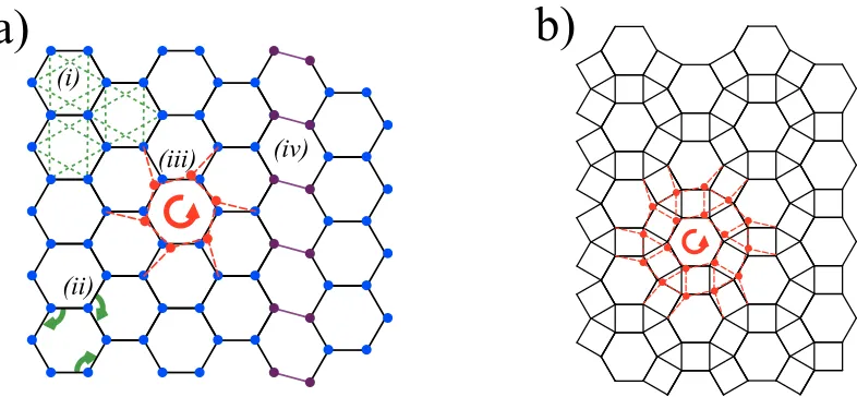
Figure 2.1: (Color Online) (a) Honeycomb lattice and (b) Small Rhombitrihexagonal (SR) lattice showing N N springs with spring-constant k. Note that in (a),(i) indicates the

N N N neighbors with spring constant k′_; _(ii) _{shows nearest bond angles with the energy} cost 1₂b∗(δθ)2 for bending;(iii) shows the local mode soft to linear order in spring energy;

(iv) shows the shear mode soft to all orders. In (b), a local soft mode of the SR lattice is visualized.

tiling by hexagons, all of the constituent particles are identical, as seen in Fig. 2.1a.

Local Modes

We note that the coordination number for the honeycomb lattice is z = 3. By the

counting argument, the number of soft modes is 2N ₋ 3₂N = N₂. This is an extensive

quantity, so that local soft modes can be found. Indeed, these have been known from

studies of electron binding and sphere packing to be local rotation of the hexagons, as seen

in Fig. 2.1a. [67, 56] Since there are twice as many particles as hexagons, we thus obtain all

N/2 soft modes in the system.

We see that the extensive number of soft modes and the presence of local soft modes are

interchangeable, to linear order. Given an extensive number of soft deformations, we could

use the technique of Wannier functions with the principle of superposition of phonons to

(40)

(a) First Brillouin Zone

K _G M K

(b) KΓMK cut

ΩM ΩK

Ω

dHΩL

(c) Density of States

Figure 2.2: (Color Online) Phonon modes of the honeycomb lattice, showing (a) the entire first Brillouin zone (1stBZ) for the lowest mode when k′ = 0.02, (b)KΓMK cut for all four modes, with k′ _{= 0}_._{02 solid lines and} _k′ _{= 0 dashed lines. Note that the lowest mode, in} red, has frequency of order_∼k′ everywhere and has stationary points precisely at K,Γ and M. (c)The density of phonon states obtained by integrating over the 1stBZ. The logarithmic divergence comes from the saddle point at M and the jump discontinuity from the maximum at K.

The Dynamical Matrix

We take a= 1 without loss of generality. The expression for the dynamical matrix can

be seen in Eq. B.1. By taking its eigenvalues, we find the dispersion relation, which is

plotted in Fig.2.2(b).

The extensive number of soft deformations leads to a mode of soft phonons which is

flat (and whose energy is zero) over the entire 1stBZ. This is consistent with the symmetry

of the system, which dictates that near the origin Γ, the dispersion must be isotropic.

The other phonon mode, corresponding to longitudinal compression, rises as expected,

ω _≈CLq = q

k

8q. Since the lattice has two particles per unit cell, ρ = 4 √

3

3 and the bulk

modulus isB = sqrt₆3k. The other two modes are gapped, with ω=√3k at Γ.

The NNN interactions result in additional terms in the dynamical matrix, seen in Eq.

B.4. These terms guarantee mechanical rigidity and the entire two-dimensional zero-energy

mode must be lifted. This results in a qualitative change in the nature of the lowest mode.

Instead of being constant, it has finite energies away from the origin of order ω _∼ √k′_.

This necessarily leads to stationary points in the dispersion relation. In fact, within a single

Brillouin zone there is a minimum, a maximum and a saddle.

(41)

lon-gitudinal (B = √₆3(k+ 6k′_{)), with the dispersion} _ω _≈ q3k′

8 q and thus µ =

√ 3k′

2 . Point

M is a saddle, with the dispersion ω2

M ≈ 2k′ +13k

′

8 δqx2− 3k

′

8 δqy2. Point K is a maximum,

ω2

K ≈ 92k′−9k

′

8 δq2. These later two points correspond to the Van Hove singularities seen

in the DOS.

If instead we consider the bending rigidity of the hexagon (Fig. 2.1a), we get a very

similar picture. While the dynamical matrix expression differs from the one forD′(q), the

above expansions near the symmetry point will still hold, given that 4b∗_→k′.

Density of States

The DOS for the lowest mode thus has a Debye rise, a logarithmic singularity at ω =

√

2k′ _{and a jump to zero at}_ω₌p

9k′_/_{2 (Fig. 2.2(c)). This is quite reminiscent of the DOS}

of a stable lattice with spring constantk′. The DOS for the longitudinal mode has a similar

behavior, but with ω _∼ k. This separation of energy scales gives the dispersion a simple

structure, and there is none of the richness seen below in isostatic systems.

Conclusions

There is vanishing critical frequency scale in the honeycomb lattice, with ω∗ _∼ √k′_.

However, since the modes are all isotropic at large scales, no meaningful divergent length

can be extracted from this model. Thus, no continuous transition takes place here, and the

contact number jumps from far above isostaticity to far below atk′ = 0.

2.2.1 Small Rhombitrihexagonal Lattice

Another lattice which has very similar behavior to the honeycomb can be obtained from

the Small Rhombitrihexagonal (SR) tiling of the plane (Fig. 2.1b). It has the same spatial

symmetry group, and indeed can be seen as a honeycomb lattice decorated with triangles

at each vertex.

Using Maxwell counting, we might expect sincez= 4 that the lattice would be isostatic.

(42)

them from giving independent constraints on the system. The rotations of the hexagons,

simple extension of the local soft modes of the honeycomb lattice, which in the SR lattice

involve 18 particles, are still soft to linear order. (Fig. 2.1b)

The dispersion relation for the SR lattice looks quite similar to that of the honeycomb

lattice, though there are 12 modes total and three withω(q=0) = 0. The latter correspond

to the two acoustic phonon modes, which in this case give large elastic moduli,µandB _∼k.

The third mode, an optical phonon, corresponds to soft rotations. We expect such mode

structure due to the presence of triangles. Defined by their three sides, they do not allow

a soft transverse phonon, which is affine in the limit q_→ 0. Triangles can only participate

in soft modes through their rotational degrees of freedom. However, apart from this detail,

this structure is essentially that of the honeycomb lattice.

2.3 Square Lattice

(a) Square Lattice (b) Soft Modes and Next-Nearest Neighbors of the Square Lattice

(43)

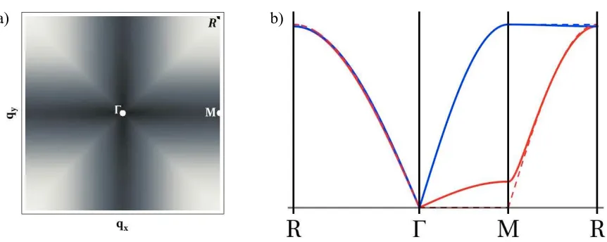
Figure 2.4: (Color Online) Phonon dispersion of the square lattice, with (a) the first Bril-louin Zone showing the lowest energy mode withk′ _{= 0}_._{02, where the softer quasi-isostatic} directions are evident and (b) the RΓMR cut, showing both of the modes atk= 0.02 (solid lines) and k′= 0 (dashed lines). The isostatic mode can be seen in red.

(44)

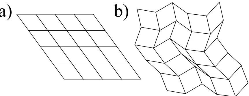
Figure 2.6: (a) The affine shear soft mode of the square lattice, signifying µ _≡ 0. (b) A random distortion of the square lattice costing zero energy in the isostatic case. Note that while (a) is a possible ground state whenk′ _<_{0, (b) is not. not correspond to a}

2.3.1 Isostatic Dynamical Matrix

The square lattice (Fig. 2.3) dynamical matrix has a simple 2x2 structure as seen in

Eq. B.6. Each mode corresponds to the displacement vector of the single particle within

the unit cell.

In order to understand the expression more intuitively, we expand in powers ofqaround

the point Γ, orq=0,

D◦(q) =k



 

q2

x 0

0 q2

y 



 (2.1)

where the lattice spacing a= 1.

By symmetry the linear elastic theory must be of the form in Eq. 1.11, so we see that

the only non-zero modulus is C11 = k, while C12 = C44 = 0. This signifies some form of

instability. Note thatC11is essentially a bulk modulus for the square lattice, and it is finite

due to the local force balance on each particle when isotropic pressure is applied.

By looking at the stability equation without external stress, Eq. 1.7 with σij = 0, for

this form of linear elasticity, we can better understand for the nature of this instability.

This reduces to two equations,

(45)

so that the displacements must be of the form

ux=cx0(y) +cx1(y)x (2.3)

uy =cy0(x) +c

y

1(x)y (2.4)

where c are arbitrary functions specified by the initial conditions. Thus, suppose we have

a rectangular portion of the lattice with free boundary conditions,σijnj = 0, where nj are

components of the surface normal. Then, e.g. at u(0, y), the condition uxx = cx1(y) = 0

must be met, and similarlycy₁(x) = 0 atu(x,0). However,cx₀(y) andcy₀(x) remain arbitrary.

In other words, the configurations are only uniquely determined if the displacements at the

boundary is specified, signifying the presence of soft modes.

Isostatic Modes

The nullspace of D◦ allows us to determine the soft modes at the largest wavelengths. We see that the linesqx= 0 andqy = 0 in the 1stBZ correspond to the soft modesu= (1,0)

and u= (0,1), respectively. Thus we see two lines of soft modes, corresponding to shear in

certain direction. Away from that, the dispersion has a one-dimensional nature, having a

knife-edge shape seen in Fig. 2.5a. Some possible deformations can be seen in Fig. 2.6.

For a finite lattice, we can obtain an exact count using the extended Maxwell counting

argument. In the case of free boundary conditions (B.C.s) in an Nx ×Ny lattice, where

Nx,y signify the number of particles along the x and y axes, respectively, no states of self

stress are present. There are thus 2NxNy−Nx−Ny bonds andNxNy particles, so that the

Maxwell count gives Nx+Ny−3 soft modes. While this lattice with periodic B.C.s has

extra bonds, they are all redundant, each resulting in a state of self stress. Thus, by the

extended Maxwell count in Sec.1.7, NB−S = 2NxNy−Nx−Ny and the number of soft

Soft Lattices

University of Pennsylvania

ScholarlyCommons

Publicly Accessible Penn Dissertations

Summer 8-12-2011

Soft Lattices

Anton Souslov

Follow this and additional works at:

http://repository.upenn.edu/edissertations

Part of the

Condensed Matter Physics Commons

Recommended Citation

Soft Lattices

Contents

List of Tables

List of Figures

Chapter 1

Motivation and Background

1.1

Introduction

1.2

Jamming

1.3

Isostaticity

1.4

Semi-Flexible Polymer Gels

1.5

Linear Elasticity

1.6

Structural Phase Transitions and Beyond

1.7

Beyond Maxwell Counting

1.8

Spring Lattice Models

1.9

A Survey of Lattices Considered

1.10

Stabilizing Terms

1.11

Finite Mechanisms as Deformations

1.12

Isostatic Phase Transitions

Chapter 2

2D Lattices

2.1

The Hyper-Isostatic Triangular Lattice

2.2

The Sub-Isostatic Honeycomb Lattice

2.3

Square Lattice