Gene-environment interaction tests for family studies with quantitative phenotypes: A review and extension to longitudinal measures

(1)

Gene – environment interaction tests for

family studies with quantitative

phenotypes: A review and extension to

longitudinal measures

Hortensia Moreno-Macias,1,2*_{Isabelle Romieu,}3_{Stephanie J. London}4_{and Nan M. Laird}5

1_{Department of Environmental Health, Harvard School of Public Health, Boston, MA 02115, USA} 2_{Universidad Auto´noma Metropolitana Unidad Iztapalapa, Me´xico DF 09340, Me´xico}

3_{International Agency for Research on Cancer, 150 Cours Albert Thomas, 69372 Lyon CEDEX 08, France}

4_{Epidemiology Branch, National Institute of Environmental Health Sciences, National Institutes of Health, Department of Health}

and Human Services, Research Triangle Park, NC 27709, USA

5_{Department of Biostatistics, Harvard School of Public Health, Boston, MA 02115, USA}

*Correspondence to: Tel: þ55 5804 6562; Fax:þ55 5612 5682; E-mail: [email protected] Date received (in revised form): 22 April 2010

Abstract

Longitudinal studies are an important tool for analysing traits that change over time, depending on individual characteristics and environmental exposures. Complex quantitative traits, such as lung function, may change over time and appear to depend on genetic and environmental factors, as well as on potential gene – environment interactions. There is a growing interest in modelling both marginal genetic effects and gene – environment inter-actions. In an admixed population, the use of traditional statistical models may fail to adjust for confounding by ethnicity, leading to bias in the genetic effect estimates. A variety of methods have been developed to account for the genetic substructure of human populations. Family-based designs provide an important resource for avoiding confounding due to admixture. To date, however, most genetic analyses have been applied to cross-sectional designs. In this paper, we propose a methodology which aims to improve the assessment of main genetic effect and gene – environment interaction effects by combining the advantages of both longitudinal studies for continu-ous phenotypes, and the family-based designs. This approach is based on an extension of ordinary linear mixed models for quantitative phenotypes, which incorporates information from a case – parent design. Our results indicate that use of this method allows both main genetic and gene – environment interaction effects to be estimated without bias, even in the presence of population substructure.

Keywords:gene – environment interaction, longitudinal phenotypes, power, bias, population substructure

Introduction

In spite of the multiple efforts to find genetic factors conferring susceptibility to complex diseases, the success of genetic association studies is still hampered by the difficulty in replicating findings in different populations. Among the plausible explanations for this lack of replication is the fact that the effects of environmental factors, which can interact with

genetic factors, are not always taken into

consider-ation.1 There is an increasing interest in studying

different susceptibilities to environmental factors in subjects with different genotypes; however, power and bias issues with regard to the statistical estimation of gene–environment interaction effects persist.

High-quality information about individual

environmental exposure is crucial for the

PRIMARY RESEARCH

(2)

assessment of gene – environment interactions.2 Failure to measure changes in exposure levels over time could lead to an underestimation of the role of the environment in the interaction. Repeated measurements of the temporal relation-ship between an outcome and the exposure may overcome such a problem when both the endpoint and the exposure are time-dependent variables. In addition, potential misclassification due to ambi-guity in the definition of complex diseases may be avoided through the measurement of quantitative disease-related phenotypes as the outcomes of interest. For example, quantifying the decrements in lung function over time through repeated spiro-metric tests may provide insights into the pathogen-esis of chronic obstructive pulmonary disease (COPD) or asthma. Many disease ‘predictor’ phe-notypes are thought to change within-subject because of both environmental and genetic factors, and of their potential interactions over time.

On the genetic side, population substructure is an important practical issue for genetic association studies. When the study population is not a collec-tion of randomly mating individuals, several dis-crete subgroups that are genetically different may be identified; the collection of these subpopulations is referred to as population substructure or

stratifi-cation.3 Moreover, disease prevalence also tends to

differ among these subgroups.4 Consequently,

without stratification adjustment, allele frequency can appear to be associated with the disease, regardless of whether the genotype has a functional effect on that health outcome or not. By contrast, when the genotype distribution is homogeneous among groups, population substructure may not be an issue. For example, if people are randomly assigned to treatment groups, it is expected that

those groups will be genetically similar. If,

additionally, there are no differences in the response to treatment among the different subgroups, bias due to population substructure is unlikely.

Another source of spurious associations is popu-lation admixture, which refers to the mixture of different ancestries; that is, people from different ethnic groups interbreed, so the genome of the new generations is a combination of genotypes of the

original ancestry groups, and, consequently, in some genes, allele frequencies are not homogeneously dis-tributed in the study population. For example, it has

been recognised that Latino populations have

varying proportions of African, Native American

and European ancestry.5 Like population

substruc-ture, if the risk of disease depends on ancestry, a high risk of disease may be erroneously associated with a high allele frequency; thus, in admixed popu-lations, ethnicity may confound associations between genotype and outcome and assessment of gene by environment interactions. The direction of the con-founding could be positive or negative. Therefore, to identify true associations, population substructure must be taken into account in the analysis.

With the increasing availability of genetic data, there is a growing interest in modelling both mar-ginal genetic effects and gene – environment inter-actions. Inclusion of interactions, when they exist, can increase the statistical power of detecting both

genetic and environmental effects.6Traditional

stat-istical models for detecting significant main effects and interactions may not be completely adequate for studying genetics in admixed or stratified popu-lations, however.

A variety of methods have been developed to account for the genetic substructure of human

populations.7 Family-based designs provide an

important resource for avoiding confounding due

to admixture.8 The simplest design for testing

association is the case – parent (or trio) design because it uses genotypes from an affected off-spring, the case, and his/her two parents. The outcome is measured, however, only in the off-spring. Many of these methods have been devel-oped for cross-sectional designs, but can be applied to repeated measurements through the two-step modelling approach. The first step consists of calcu-lating the slope between the longitudinal outcome and the time-dependent environmental exposure; thus, we calculate a single individual endpoint, the slope, for each subject. In the second step, the genetic methods for cross-sectional studies, where

the slope is the single outcome, can be applied.9

In this paper, we first provide a short review of different approaches for studying gene– environment

Gene – environment interaction tests for family studies with quantitative phenotypes PRIMARY RESEARCH

(3)

interactions for quantitative traits, and then propose a method that aims to improve the assessment of main and gene –environment interaction effects by com-bining the advantages of both longitudinal studies for continuous phenotypes and the family-based designs. This approach is based on an extension of ordinary linear mixed models (OLMM) for quanti-tative phenotypes which incorporates information from a case– parent design. We call the model the

‘adjusted linear mixed model’ (ALMM), and

through simulation methods we show that even when population stratification is present, both main genetic and gene– environment interaction effects can be estimated without bias, and that this is more powerful than the two-step modelling approach.

The broad objectives of this paper do not extend to giving technical details about the family-based approach and its extensions, or to giving an extensive explanation about linear mixed models. Rather, we present what we consider to be a widely applicable method for correctly assessing the main genetic effect and gene – environment inter-actions for time-dependent quantitative traits in stratified populations. For this purpose, we use simulated repeated measurements of forced expira-tory flow between 75 per cent and 25 per cent of

vital capacity (FEF25 – 75) ie (lung function) on

asth-matic children exposed to ozone pollution, based on the observed distributions in a real cohort study

conducted in Mexico City.10

In order to set the stage for our methodology, we first provide a brief overview of some existing ordinary linear regression (OLR) models for testing main genetic effects and gene – environment inter-actions in cross-sectional studies that incorporate information about parental genotype (case – parent or trio design), adjusting for admixture. We then briefly present the family-based association test (FBAT) approach, which, as a second step (after computing the slope between the outcome and the exposure), represents an alternative method for ana-lysing genetic associations over time. We next review the ordinary linear mixed models (OLMM) which are a standard approach for the analysis of longitudinal data, and present the adjusted linear mixed models (ALMM) as an extension of OLMM

combined with the adjusted cross-sectional

regression models. In order to show that the two-step modelling approach provides a valuable alternative for analysing longitudinal data, we explain the relationship between this approach and the linear mixed models. Finally, we give details about the simulation procedures and present our results and discussion.

Methods

Models for cross-sectional data with a single quantitative measure for each subject

Existing methods for testing main genetic effect and

gene–environment interactions with a single

measured outcome include (1) OLR models and extensions that aim to adjust for ethnicity by includ-ing parental genotype information in a case–parent or trio design, and (2) the FBAT approach, which

uses a score test based on a conditional likelihood.11

The OLR approach

In a genetic association analysis with quantitative traits that follow a linear model, the assessment of gene – treatment interactions may be conducted using standard linear regression models for inde-pendent subjects. Under the usual assumptions, the well known model for testing the interaction between two covariates is:

EðYijX;ZÞ ¼b0þb1Xiþb2Ziþb3XiZi

for i¼1;2;. . .n; ð1Þ

where:

n is the number of subjects in the study;

Xi is a fixed variable that translates an offspring

genotype into a numeric value; and

Zi is an observed environmental covariate, either

continuous or dichotomous.

Xi is a scalar whose value depends on the disease

model. If the locus has two alleles, A and a, the

additive model assumes that each copy of the

variant allele* ‘A’ changes the outcome in an

addi-tive amount. Thus, Xi counts the number of ‘A’

*Usually the variant allele is the less frequent.

PRIMARY RESEARCH _{Moreno-Macias}_{et al.}

(4)

alleles in the offspring genotype ðXi ¼ f0;1;2gÞ.

In the recessive model, Xi is coded as an indicator

variable for the AA genotype. As a special case,

model (2) is used for testing main genetic effects adjusted for the environmental covariate:

EðYijX;ZÞ ¼b0þb1Xiþb2Zi ð2Þ

A rejection of the null hypothesis H0 :b1 ¼0

means that the quantitative trait is associated with the alleles in the marker.

The case – parent or trio design

Unlike OLR models, family designs aim to avoid spurious associations due to population admixture. In the case – parent design, the proband is the off-spring that identifies the family for the study; the genotypes of the candidate gene are measured for all members of the trio, but the quantitative trait is measured only in the offspring. The alternative form of the OLR approach for testing main genetic effect on quantitative outcomes, where the parental genotype information is included, was

developed by Allison;12 it is based on the simplest

family-based design for testing associations, known

as the transmission disequilibrium test (TDT).13

The model is adjusted for the expected value of the offspring’s genotype conditional on the parental genotypes; thus, the adjusted version of model (2) is:

EðYijX;ZÞ ¼b0þb1ðXiEðXijgim;gifÞÞ

þb₂Zi ð3Þ

where:

gim;gif are the parental genotypes (mother and

father, respectively) and EðXijgim;gifÞ is calculated

under segregation and independent assortment assumptions using Mendel’s law. Its value depends on the mating type and the disease model.

The adjusted genotype XiEðXijgim;gifÞ is the

subject’s deviation from the family mean under

Mendel’s law. b₁ represents the within-family effect

of the gene on the outcome. As a result of centring

Xi by its expected value conditional on parental

genotypes (gim;gif), ethnicity bias is avoided, since

all possible genotypes — depending on the mating

type — are taken into account, even those that were not transmitted to the affected offspring. This strategy does not, however, necessarily prevent bias

due to other kinds of population stratification,14

such as the one that occurs when parental mating type is highly correlated with the levels of

exposure, for example. For this reason, Allison12

and Ewens et al.14 propose an alternative version of

model (3) in which the intercept, representing the

between-family component, depends on the

mating type as a fixed effect:

EðYijX;ZÞ ¼b0M þb1ðXiEðXijgim;gifÞÞ þb2Zi

¼b~₀_M þb₁Xiþb2Zi

ð4Þ

where:

~

b₀_M ¼b₀_M b₁EðXijgim;gifÞ

and M¼1, 2, 3 are the three possible mating types

with at least one heterozygous parent, including

informative families only.† Note that here and in

subsequent equations, M depends upon i via the

parental genotypes, but this is suppressed for simplicity.

It is noteworthy that since both b0M and

EðXjgim;gifÞ are constant within the mating type,

the estimation of the main genetic effect (b1)

through model (4) is completely equivalent to using model (5):

EðYijX;ZÞ ¼b0M þb1Xiþb2Zi ð5Þ

Following the same idea, Gauderman15 proposed

a likelihood ratio test (LRT) of b₁ in model (5),

although, in order to increase the power for detect-ing main genetic effects, he included the whole set of families, regardless of the heterozygous con-dition. This is called the quantitative transmission disequilibrium test with mating type indicators

(QTDTM). An extension of the QTDTM to

†

There are six different mating types: AAXAA, AAXAa, AAXaa, AaXAa, AaXaa, and aaXaa. When both parents are homozygous, the observed and conditional expected genotypes are equal and it is said that the family is not informative.

(5)

include the environmental covariate and the gene – environment interaction was also suggested by

Gauderman15 with the model:

EðYijX;ZÞ ¼b0M þb1Xiþb2Ziþb3XiZi ð6Þ

Where M¼1, 2,. . ., 6 are the six possible

mating-types.

In contrast to the relationship between models (4) and (5), model (6) is not equivalent to:

EðYijX;ZÞ ¼b0Mþb1½XiEðXijgim;gifÞ

þb2Ziþb3Zi½XiEðXijgim;gifÞ

ð7Þ

because, although b0M and EðXijgim;gifÞ are

con-stant within mating type, the environmental covari-ate (Zi) is not.

An alternative model to (7), (and an extension of Gauderman’s idea), is given by the adjusted model that we call the adjusted quantitative transmission disequilibrium test with mating-type indicators

(AQTDTM).

EðYijX;ZÞ ¼b0Mþb1½XiEðXijgim;gifÞ þb2MZi

þb₃Zi½XiEðXijgim;gifÞ ð8Þ

where now both the intercept and the slope for the environmental covariate depend on the mating type, which means that the model has been adjusted for a potential correlation between the exposure to environmental factors and the mating type. Note that now model (8) is equivalent to:

EðYijX;ZÞ ¼b0Mþb1Xiþb2MZiþb3ZiXi ð9Þ

The advantage of using models (5) and (9) is that the inclusion of an indicator variable for the mating type, rather than calculating the expected genotype, provides protection against population admixture while taking into account those situations where environmental exposure (Z) may depend on the mating type and other additional types of population

substructure.14 As usual, in (6), (7), (8) and (9), b₃

estimates the effect modification of the gene on the

environmental effect Zi and H0 :b3 ¼0 is the null

hypothesis that states the no interaction effect.

The FBAT approach

FBAT is the generalisation of the TDT for the trio design. It encompasses a broad class of statistical methods for testing genetic associations adjusting for potential admixture or stratification. Such methods are also based on extensions of the TDT and regression models, although the covariance between

genotype and phenotype is the statistic of interest.11

The general FBAT statistic has been explained

else-where.16Briefly, for nnuclear families, one offspring

in the familyiand no covariates:

x2_FBAT ¼ U

2

VarðUÞ ð10Þ

where:

U ¼X½ðYiEðYiÞÞðXiEðXijgim;gifÞÞ

for i¼1;2;. . .n;

VarðUÞ ¼X

i

ðYiEðYiÞÞ2VarðXijgim;gifÞ;

and EðXijgim;gifÞ and VarðXijgim;gifÞ are calculated

under the null hypothesis of Mendel’s law. This stat-istic follows a chi-square distribution with one degree of freedom. In addition, unlike regression models where the offspring’s genotype is assumed to be fixed and observed, the general FBAT approach considers the offspring genotype as a random variable. The general idea is first to calculate a test statistic for the association between the trait and the marker locus, and then, as a second step, the distribution of this test statistic is derived from the distribution of the off-spring genotype under the null hypothesis of no association. The distribution of the test statistic is computed conditioning on the sufficient statistic given by the parental genotype and the observed off-spring’s phenotype. Under these conditions, no assumptions about the allele frequency, the recombi-nation fraction or the penetrance function are required. Due to the fact that the general FBAT stat-istic can only test main genetic effects, and since the test statistic is based the relative size of U with respect to its standard deviation, the genetic effect is not directly estimated.

(6)

Under the philosophy of the FBAT, Vansteelandt

et al.17 proposed an extension that permits the assessment of and testing for the gene – environ-ment interaction without any assumptions about the genotype distribution and with no bias due to unmeasured ethnicity confounding through which Mendel’s laws hold. Such an extension is based on G-estimation (causal inference) methodology and is called QBAT-I; this test statistic has the same form as the general FBAT (10), although the expected genotype and the U statistic have more complex expressions. A brief presentation of both FBAT and QBAT-I can be found in Appendix 1.

FBAT and QBAT-I statistics are available from PBAT free software at http://biosun1.harvard.edu/ ~clange/pbat.htm and in the library pbatR under the R package environment.

Models for longitudinal data

Until now, we have discussed methods for analysing gene – environment interactions when a single measurement of the phenotype is available. We now turn to a discussion of methods for the analy-sis of quantitative repeated phenotype data to evalu-ate the effects of a gene and the environment over time.

In longitudinal designs, the unit of study is not each individual or each measurement, but rather the sequence of measurements on each subject. This means that the major advantage of a longi-tudinal analysis is that the so-called cohort and age effects are estimated separately; that is, differences among people in their baseline levels (cohort effects), can be discriminated from the changes over time (ageing effects) within individuals. In other words, measurements across people and repeated values across time are sources of strength. Note that cross-sectional data provide information for asses-sing only the former effect; thus, longitudinal studies tend to be more powerful than

cross-sectional studies.18

Although there are different approaches to longi-tudinal data analysis, we consider here the two most commonly used: OLMM and two-step methods.

OLMM

OLMM assumes that the vector of repeated measurements on each subject follows a linear regression model. Thus, each individual model may have subject-specific intercept and slope (the random effects) representing the different suscepti-bilities to the environmental exposure among

sub-jects. For most outcomes, variability across

individuals is greater than within-subject. This difference may be due the influence of genetic

composition.19

In general, a linear mixed-effects model satisfies:

Yij ¼a0þa1tijþa2Ziþa3Xiþa4XiZiþa5Xitij

þa6Zitijþa7XiZitijþb1iþb2itijþeij

ð11Þ

where:

i ¼1;2;3;. . .;n subjects;

j ¼1;2;3;. . .;m corresponding times at which the measurements are taken on each subject;

tij is the repeated time (or exposure) variable;

b1i is the random subject intercept effect (a0þb1i),

which varies among subjects;

b2i is the random subject slope effect ða1þb2iÞtij,

which varies among subjects;

eij is a random variable regarded as measurement or

sampling errors;

Eðb1iÞ ¼Eðb2iÞ ¼EðeijÞ ¼0

Varðb1iÞ ¼s2_b₁; Varðb2iÞ ¼s2_b₂; VarðeijÞ ¼s2;

Covðb1i;b2iÞ ¼s12;

and Xi and Zi are as previously defined. Note that

model (11) assumes that both genotype (Xi) and

environmental exposure (Zi) remain fixed over

time. However, we can take advantage of the time

variable (tij) to include an extra source of exposure

that changes across time. For example, we are

par-ticularly interested in the assessment of the

gene – environment interaction effect between the

glutathione-S-transferase M1 gene (GSTM1) and

(7)

antioxidant supplementation on lung function — FEF25 – 75— of asthmatic children exposed to ozone.

Therefore, in model (11), Xi represents the

indi-vidual GSTM1 genotype and Zi is a dichotomous

variable that denotes the antioxidant supple-mentation group which was randomly assigned at baseline and remained fixed during follow-up, and which since ozone is a time-dependent variable,

can be represented by tij. This is a model with

random intercept and random slope on ozone. As for ordinary linear regression models in cross-sectional studies, OLMM assumes independent subjects and does not account for population admixture. Therefore, in order to avoid potential estimation bias, it is necessary to adjust for ethnicity.

ALMM

The ALMM form is a straightforward extension of the approaches presented for the cross-sectional

designs. That is, following the ideas of Allison,12

Ewens et al.14 and Gauderman,15 model (12) can

be rewritten using the indicator variables for the

mating type and the offspring’s conditional

expected genotype:

FEF2575ij ¼a0Mþa1Mtijþa2Zi

þa3½XiEðXijgim;gifÞ

þa4½XiEðXijgim;gifÞZi

þa5½XiEðXijgim;gifÞtijþa6MZitij

þa7½XiEðXijgim;gifÞZitij

þb1iþb2itijþeij

ð12Þ

wherei, j,b1i, b2i,eij are as defined for (11); Xi

rep-resents the GSTM1 genotype; Zi denotes the

anti-oxidant supplementation group; tij represents the

ozone exposure and M¼f1,2,. . ., 6g are the six

possible mating types. This model is an extension of (11) and is able to control for population admixture and for any dependence of the environmental exposure on mating type. Once again, using an indi-cator variable for the mating type prevents controls for other potential sources of population structure.

Note that, as in model (8), the simplest, but equivalent, expression for the above model that does not need the calculation of the expected gen-otype is given by:

FEF2575ij ¼a0M þa1Mtijþa2Ziþa3Xiþa4XiZi

þa5Xitijþa6MZitijþa7XiZitij

þb1iþb2itijþeij

ð13Þ

Through this model, the main genetic and environmental effects and gene – environment inter-actions can be assessed using standard statistical soft-ware. Additional advantages of this model are that genetic and longitudinal effects are estimated simul-taneously; thus, parameters are mutually adjusted

for each other9and within- and between-individual

variabilities are taken into account. Moreover, the model can be adjusted by other covariates, such as gender and age at baseline, or even by smooth functions of variables which have non-linear associ-ation with the outcome. In particular, in the example, two sources of environmental exposures — supplementation treatment (a constant) and ozone (which is time dependent) — are included. Computationally, longitudinal models require more complex algorithms than those corresponding to cross-sectional designs; however, this is no longer a problem for the users of statistical packages. Appendix 1 includes the R code for estimating the effects of model (13).

Two-step modelling approach

As the term implies, this approach includes two separate steps. In the first step, it is assumed that the

repeated measures on subject i, are independent

and follow a linear regression model. Therefore, the individual intercept and slope are estimated by an ordinary linear regression model:

Yij ¼g0iþg1itijþeij ð14Þ

Therefore, different regression coefficients (g₀

intercept and g₁ slope) correspond to different

individuals. For example, with the lung function

data, the outcome is the repeated FEF25 – 75 and g1

(8)

represents individual susceptibility to ozone over time. Thus, the longitudinal observations are

reduced to one summary statistic per subject.20 The

second step includes the genetic analysis where these slopes are the single outcome for each person. This approach has been frequently used in

segre-gation, linkage and association analysis.9 The R

code for these models is included in Appendix 1. It is interesting to note the close relationship between the coefficients in the two-step model and the respective coefficients in a linear mixed model. That is, by definition, from the ordinary linear regression model (14):

slopei ¼g1i ¼

P

jðYijYiÞðtijtiÞ

P

jðtijtiÞ

2

whereYij is given by (11) and

Yi ¼a0þa1tiþa2Ziþa3Xiþa4XiZiþa5Xiti

þa6Zitiþa7XiZitiþb1iþb2itiþei

Thus, it is straightforward to show that

slopei ¼a1þa5Xiþa6Ziþa7XiZiþei

)EðslopeijX;ZÞ ¼a1þa5Xi

þa6Ziþa7XiZi

This therefore enables one to relate the a

coeffi-cients of the linear mixed model to the b

coeffi-cients of the ordinary linear regression model given

by (1) as follows: b₁ ¼a5 and b3¼a7

represent-ing the main genetic effect and the gene – treatment interaction on the slope, respectively.

This approach is remarkably similar to that of mixed models, although longitudinal and genetic

effects are not jointly estimated, and

time-dependent covariates need to be summarised in one measurement — the mean or the median, for example — in order to be included in the analysis. Computationally, this procedure is simpler than mixed models, and any elemental statistical package will suffice for conducting the analysis.

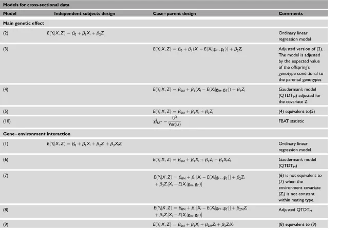
Table 1 summarises the different models included in this section.

Simulations

Here, we address differences in the analytical approaches, in terms of both bias and power, for detecting main genetic effects and gene – environ-ment interactions using simulations.

In order to compare the different methods pre-sented, we simulated data with similar

character-istics to those in the study by Romieu et al.10

Briefly, this study was a randomised trial using a double-blinded and longitudinal design, including antioxidant supplementation for asthmatic children who were residents of Mexico City and therefore exposed to ozone pollution. There were 12

repeated measures for both FEF25 – 75 and ozone.

The deletion polymorphism of GSTM1, absent

versus present, was determined for each child and, through a stratified analysis, evidence for inter-action between the antioxidant treatment

(dichoto-mous and fixed variable) and the GSTM1

genotype was seen for the effect of ozone on lung function.

For our simulations, 12 repeated measures of

lung function (FEF25 – 75) were generated for each

offspring with a mean vector given by a linear mixed model conditional on treatment, genotype and ozone level, assuming an additive (or recessive) disease model (15). An error vector was added to each mean by drawing from a multivariate normal distribution. The variance– covariance matrix of the errors was assumed to be equal to the observed var-iance– covariance matrix among the residuals in the real data, where model (15) was fit to the repeated FEF25 – 75measurements.

For the purpose of using the family-based approach, samples of independent trios were simu-lated. Each parent was randomly assigned a geno-type assuming the Hardy – Weinberg equilibrium, while each offspring was assigned a genotype assuming Mendel’s law. Treatment (Z) was ran-domly and independently assigned for each subject

i with a 50 per cent probability for supplement or

placebo group. Both additive and recessive disease models were considered.

With regard to the population stratification, two different situations were considered: the first one assumed a homogeneous population (HP), where

(9)

Table 1. Regression models included in the paper . The ‘Model’ column refers to the number that identifies each model in the paper.

Models for cross-sectional data

Model Independent subjects design Case – parent design Comments

Main genetic effect

(2) EðYijX;ZÞ ¼b0þb1Xiþb2Zi Ordinary linear

regression model

(3) EðYijX;ZÞ ¼b0þb1ðXiEðXijgim;gifÞÞ þb2Zi Adjusted version of (2).

The model is adjusted by the expected value of the offspring’s genotype conditional to the parental genotypes

(4) EðYijX;ZÞ ¼b0Mþb1ðXiEðXijgim;gifÞÞ þb2Zi Gauderman’s model

(QTDTM) adjusted for

the covariate Z

(5) EðYijX;ZÞ ¼b0Mþb1Xiþb2Zi (4) equivalent to(5)

(10) x2

FBAT ¼

U2

VarðUÞ FBAT statistic

Gene–environment interaction

(1) EðYijX;ZÞ ¼b0þb1Xiþb2Ziþb3XiZi Ordinary linear

regression model

(6) EðYijX;ZÞ ¼b0Mþb1Xiþb2Ziþb3XiZi Gauderman’s model

(QTDTM)

(7) _E_ð_Y

ijX;ZÞ ¼b0Mþb1½XiEðXijgim;gifÞ þb2Zi

þb₃Zi½XiEðXijgim;gifÞ

(6) is not equivalent to (7) when the

environment covariate (Zi) is not constant

within mating type.

(8) EðYijX;ZÞ ¼b0Mþb1½XiEðXijgim;gifÞ þb2MZi

þb₃Zi½XiEðXijgim;gifÞ

Adjusted QTDTM

(9) EðYijX;ZÞ ¼b0Mþb1Xiþb2MZiþb3ZiXi (8) equivalent to (9)

Continued

PRIMAR

Y

RESE

ARCH

Mor

eno-Ma

cias

et

al.

310

#

H

E

N

R

Y

S

T

E

W

A

R

T

P

U

B

L

IC

A

T

IO

N

S

1479

–

7364.

HUMAN

GENO

MICS

.

V

OL

4.

NO

5.

302

–

326

JUNE

(10)

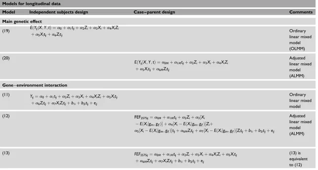
Table 1. Continued

Model Independent subjects design Case – parent design Comments

Main genetic effect

(19) EðYijjX;Y;tÞ ¼a0þa1tijþa2Ziþa3Xiþa4XiZi

þa5Xitijþa6Zitij

Ordinary linear mixed model (OLMM)

(20)

EðYijjX;Y;tÞ ¼a0Mþa1Mtijþa2Ziþa3Xiþa4XiZi

þa5Xitijþa6MZitij

Adjusted linear mixed model (ALMM)

(11) _Y

ij¼a0þa1tijþa2Ziþa3Xiþa4XiZiþa5Xitij

þa6Zitijþa7XiZitijþb1iþb2itijþeij

Ordinary linear mixed model

(12) _FEF2575_ij_¼_a₀_M_þ_a₁_M_t_ij_þ_a₂_Z_i_þ_a₃_½_X_i

EðXijgim;gifÞ þa4½XiEðXijgim;gifÞZiþ

a5½XiEðXijgim;gifÞtijþa6MZitijþa7½XiEðXijgim;gifÞZitijþb1iþb2itijþeij

Adjusted linear mixed model (ALMM)

(13) _FEF

2575ij¼a0Mþa1Mtijþa2Ziþa3Xiþa4XiZiþa5Xitij

þa6MZitijþa7XiZitijþb1iþb2itijþeij

(13) is equivalent to (12)

Xiis a fixed variable that translates an offspring genotype to a numerical value;Ziis an observed environmental covariate, either continuous or dichotomous;gim;gif are the parental genotypes (mother and father,

respectively);EðXijgim;gifÞis calculated under segregation and independent assortment assumptions using Mendel’s law;M¼1, 2,. . .,6 are the six possible mating types;i¼1;2;3;. . .;nsubjects;j¼1;2;3;. . .;m

measurement occasions into the subject;tijis the repeated time (or exposure) variable;

b1iis the random subject intercept effect; (a0þb1i) varies among subjects;b2iis the random subject slope effect:ða1þb2iÞtijvaries among subjects;eijis a random variable regarded as measurement or sampling errors.

Gene

–

envir

onment

inter

action

tes

ts

for

fa

m

ily

stud

ies

with

quantita

tiv

e

phen

otypes

PRIMAR

Y

RESE

ARCH

#

H

E

N

R

Y

S

T

E

W

A

R

T

P

U

B

L

IC

A

T

IO

N

S

1479

–

7364

.

HUMAN

GEN

OMICS

.

V

OL

4.

NO

5.

302

–

326

JUNE

2010

(11)

the observed allele frequency for GSTM1,

PðaÞ ¼0:4 and PðAÞ ¼0:6,‡ was used for

simulat-ing the genotypes. The generatsimulat-ing model we used had the following form:

EðYijjX;Z;tÞ ¼a0þa1tijþa2Ziþa3Xiþa4XiZi

þa5Xitijþa6Zitijþa7XiZitij

ð15Þ

Where: tij represents the time-dependent ozone

exposure; Zi is a dichotomous variable representing

the treatment group and Xi is either a continuous

variable counting the copy variant number of

GSTM1 (0, 1 or 2) in the additive disease model or a dummy variable in the recessive case. The par-ameters are:

a0 ¼1:8; a1¼ 0:8; a2¼ 0:2; a3 ¼ 0:05; a4 ¼0:2; a5¼0:5; a6 ¼0:6;a7 ¼1:0 a0,a1,a2,a3,a4are equal to the corresponding estimates obtained through a linear mixed model with random intercept and random slope on ozone applied to the original dataset. With the only aim to simulate situations where the effects are clearly identified without using large samples but rather looking at the differences between the methods,

a5, a6, a7 were magnified. Assigned values to a5,

a6, ða7Þ try to mimic the respective effects found

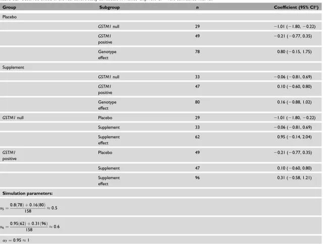
in the stratified analysis reported by Romieu et al.10

Specifically, the genotype effect for each part per billion ( ppb) of ozone was 0.8 ml/s in the placebo

group (n¼78 subjects) and 0.16 ml/s in the

sup-plement group (n¼80); thus, the main genetic

effect was taken as the rounded weighted average effect, while ignoring the supplement effect. The same procedure was applied to calculating the main treatment effect. Finally, since the effect of

antioxi-dants was stronger in the GSTM1 null genotype

group (0.95 ml/s), and there was no significant

effect in the GSTM1-positive group, the coefficient

for the gene – treatment interaction on the lung

function – ozone relationship was rounded to 1.0. Table S1 summarises the models used in the simu-lation process and Table S2 shows the observed effects in the real cohort study conducted in Mexico City.

The second situation presumes a stratified popu-lation (AP) with a 50/50 mix coming from two populations with different allele frequencies and different susceptibilities: P1ðAÞ ¼0:4;P1ðaÞ ¼0:6

andP2ðAÞ ¼0:8;P2ðaÞ ¼0:2. Note that, on average,

the combined population has the same allele fre-quencies as the homogeneous one. With the purpose of simulating differential susceptibilities to ozone and supplementation, although allowing the bias assessment for the main genetic and interaction

effects, generating model (15) differs in b₀ and b₆

coefficients (based on the observed percentiles). That is, in the first population, the observed 95th

percentile for FEF25 – 75 (a0 ¼3:3) was used as the

intercept, and no treatment effect on the slope

a6 ¼0 was assumed. On the other hand, in the

second population, the 5th percentile (a0 ¼0:75)

was taken as the intercept, and a strong treatment

effect on the slope was assumed, a6 ¼2 (meaning

that 20 ml/s/10 ppb decreased lung function, on average, in the placebo group in comparison with the supplement group). The variance– covariance matrix was constant over the different simulated samples.

Regarding the genetic effect, two different scen-arios were considered. The first scenario represents situations where the variability in the outcome may be attributable just to the main effect of the gene and the treatment, meaning that there is no gene –

treatment interaction effect ða7 ¼0Þ in the

gener-ating model (15). The second scenario assumes that all genetic, treatment and gene – treatment interaction are present in the true model.

Assessment of main genetic effect

The first scenario, where there is no gene –

treat-ment interaction (a7 ¼0), was used for testing the

main genetic effect, adjusted by treatment effect. Under the two-step modelling approach, the slope between the outcome and ozone was first computed. In the second step, the ordinary linear

regression model (16), the AQTDTM (17) model

‡ Although alleleAwas not the less frequent, it was considered the variant allele because, in the original study, children with genotype AA were classified asGSTM1null (no copy), and those with genotypesaA(one copy) andaa(two copies) were consideredGSTM1positive.

(12)

and the FBAT statistic (18) were used for testing the null hypothesis of no main genetic effect (H0 :b1 ¼0).

EðslopeijX;ZÞ ¼b0þb1Xiþb2Zi; ð16Þ

EðslopeijX;ZÞ ¼b0Mþb1Xiþb2Zi ð17Þ

x2_FBAT ¼

P

½ðslopeiEðslopeiÞÞ

ðXiEðXijgim;gifÞÞ

P

iðslopeiEðslopeiÞÞ

2

VarðXijgim;gifÞ

ð18Þ

The corresponding null hypothesis when using

longitudinal outcomes H0 :a5 ¼0 was tested

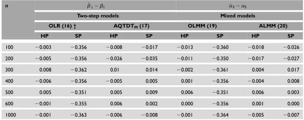
Table 2. Bias results for main genetic effect assessment comparing ordinary statistical methods (OLR and OLMM) to family-based

methods (AQTDTMand ALMM) under homogeneous (HP) and stratified (SP) populations. Each time,ncases were simulated with

parametersb1¼a5¼0.5. Simulations are based on the additive genetic model. †¼number that identifies each model in the paper.

n b^₁b₁ a^5a5

Two-step models Mixed models

OLR (16) † AQTDTM(17) OLMM (19) ALMM (20)

HP SP HP SP HP SP HP SP

100 20.003 20.356 20.008 20.017 20.013 20.360 20.018 20.026

200 20.005 20.356 20.026 20.035 20.011 20.350 20.017 20.027

300 0.008 20.362 0.01 0.014 20.002 20.361 0.004 0.017

400 20.006 20.356 20.005 0.005 0.001 20.356 20.004 0.008

500 0.005 20.351 0.005 0.009 0.006 20.351 0.006 0.003

600 20.001 20.355 0.006 0.002 0.000 20.356 0.001 0.000

1000 20.001 20.363 20.006 20.008 20.001 20.364 20.005 20.007

OLR, ordinary linear regression; OLMM, ordinary linear mixed models; ALMM, adjusted linear mixed models; AQTDTM, adjusted quantitative transmission disequilibrium test with mating type indicators

Table 3. Bias results for gene – environment interaction effect assessment comparing ordinary statistical methods (OLR and OLMM) to

family-based methods (AQTDTMand ALMM) under homogeneous (HP) and stratified (SP) populations. Each time,ncases were simulated

with parametersb3¼a7¼1. Simulations are based on the additive genetic model. †¼number that identifies each model in the paper.

n b^₃b₃ a^7a7

Two-step models Mixed models

OLR (21) † AQTDTM(22) OLMM (23) ALMM (24)

HP SP HP SP HP SP HP SP

100 0.001 20.687 20.013 0.066 20.013 20.719 0.008 0.029

200 0.001 20.745 0.034 20.008 0.007 20.738 20.008 20.007

300 20.008 20.713 0.007 0.004 20.005 20.716 0.011 0.009

400 0.002 20.719 0.012 0.01 0.005 20.711 0.014 0.016

500 0.01 20.729 0.000 20.027 20.001 20.725 0.011 20.006

600 0.011 20.697 0.014 0.008 0.012 20.704 0.016 0.005

1000 0.003 20.728 0.007 20.018 0.052 20.730 0.011 20.075

OLR, ordinary linear regression; OLMM, ordinary linear mixed models; ALMM, adjusted linear mixed models; AQTDTM, adjusted quantitative transmission disequilibrium test with mating type indicators

(13)

through ordinary and adjusted linear mixed models; that is:

EðYijjX;Y;tÞ ¼a0þa1tijþa2Ziþa3Xiþa4XiZi

þa5Xitijþa6Zitij

ð19Þ

and

EðYijjX;Y;tÞ ¼a0Mþa1Mtijþa2Ziþa3Xi

þa4XiZiþa5Xitijþa6MZitij

ð20Þ

For the purpose of comparison, statistics based on model (16) will be referred to as OLR, those

based on (17) will be referred to as the QTDTM,

those based on (19) will be referred as OLMM and those based on (20) will be referred as ALMM.

Assessment of gene – environment interaction

Using the same idea, the second scenario, where

a7 ¼1 in the generating model, was used for

asses-sing the interaction effect through a one degree of freedom test.

Assuming one outcome per individual, in the two-step modelling approach, the null hypothesis

H0 :b3 ¼0, was tested using (21), (22) and the

QBAT-I statistic:

EðslopeijX;ZÞ ¼b0þb1Xiþb2Ziþb3ZiXi

ð21Þ

EðslopeijX;ZÞ ¼b0M þb1Xiþb2MZiþb3ZiXi

ð22Þ

For repeated measurements, the corresponding

null hypothesis H0 :a7 ¼0 was tested using the

OLMM and ALMM models respectively:

EðYijjX;Z;tÞ ¼a0þa1tijþa2Ziþa3Xiþa4XiZi

þa5Xitijþa6Zitijþa7XiZitij

ð23Þ

and

EðYijjX;Y;tÞ ¼a0M þa1Mtijþa2Ziþa3Xi

þa4XiZiþa5Xitijþa6MZitij

þa7XiZitij

ð24Þ

For the purpose of comparison, statistics based on model (21) will be referred to as OLR, those based

on (22) will be referred to as the adjusted AQTDTM,

those based on (23) will be referred as OLMM and those based on (24) will be referred as ALMM.

The empirical power for each test was estimated as the percentage of occasions on which the null

hypothesis was rejected at a significance level a

0.05 for a two-sided test. In each simulation study, 1,000 independent replicate datasets were generated.

Each dataset consisted of n (n¼100, 200, 300, 400,

500, 600 and 1,000) complete and independent trios. Bias was calculated as the average of the differ-ence between the estimator and the true parameter value (b^ b).

Results

Estimation bias

In order to look at the differences among methods, the estimation bias for the main genetic effects and gene – environment estimation was computed under both population conditions, homogeneous (HP) and stratified (SP) populations. Table 2 shows the resultant bias for the four methods, with two columns per method (HP and SP). When there is

no ethnicity confounding (HP), all methods

(OLR, AQTDTM, OLMM and ALMM) for

esti-mating main effects are unbiased, regardless of the design analysis (independent subjects or trios) or the modelling approach (two-step or longitudinal data). By contrast, when the population is stratified, the selection of the design is crucial. In other words, while estimators obtained from the case – parent design are unbiased, models using indepen-dent subjects underestimate the effects by around 0.36 units. Note that, regardless of the modelling approach, both designs provide similar results.

(14)

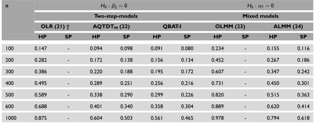
As in the main genetic effect assessment, the esti-mation of the gene – environment interaction also depends strongly on the design of the study when there is population stratification. In this case, when using ordinary statistical methods, the interaction effect was also underestimated by about 0.72 units, but with a homogeneous population the design is not relevant in terms of bias (Table 3).

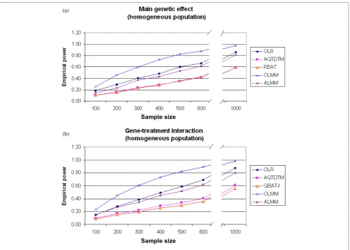
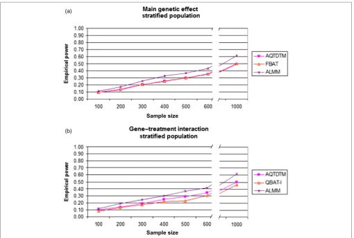
Empirical power

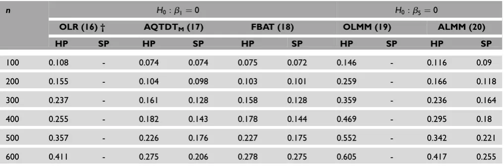
Since power comparisons among biased and unbiased methods cannot be fair, the power of OLR and OLMM under population stratification was not com-puted. Regarding genetically homogeneous popu-lations, in both main genetic and gene–treatment

interaction effects, ordinary regression models are the most powerful methods (Figures 1 and 2). Moreover, and as was expected, the use of repeated measures (OLMM) is more powerful than the use of a single measure (OLR). Note that, among the family-based models, ALMM is the most powerful and that FBAT

or QBAT-I statistics and AQTDTM are equivalent

with regard to power.

When the population is genetically mixed, all methods, regardless of the modelling approach or the design, lose power in comparison with the setting where the population is homogeneous (Tables 4 and 5). Once again, ALMM is the most powerful method for detecting main genetic or the interaction effects. In other words, the modelling

Figure 1. (a). Empirical power results for main genetic effect assessment comparing different methods under the assumption of a

homogeneous population. Simulations are based on the sample size as indicated in the plot and the additive genetic model. (b) Empirical power results for gene – environment interaction effect comparing different methods under the assumption of a homogeneous population. Simulations are based on the sample size as indicated in the plot and the additive genetic model.

(15)

approach may be crucial, in terms of power, for conducting the association analysis.

Additive versus recessive disease models

In the recessive model, the same relationship among methods is observed, although the addi-tive model is always more powerful than the reces-sive one, regardless of the testing approach. The data are shown in the supplementary tables. This may be related to the fact that in the additive

model, X has a wider range of variation, whereas

in the recessive one, X is an indicator variable. In

addition, the number of informative families for FBAT statistics is always larger when the additive disease model is assumed, while the number with a

causal genetic mutation is smaller under the reces-sive model assumption.

In summary, if the study population is geneti-cally homogeneous, an independent subjects

design provides unbiased genetic estimates,

regardless of the modelling approach, and offers the most powerful tests as well. The models that use repeated measurements are even more power-ful than those using one single outcome per subject, however. When the study population is stratified, using OLR or OLMM can result in

spurious associations; therefore, in order to

control for potential population admixture or stratification, family-based designs are strongly recommended. ALMM is more powerful than

QTDTM and FBAT statistics.

Figure 2. (a). Empirical power results for the main genetic effect assessment comparing different methods under the assumption of a

stratified population. Simulations are based on the sample size as indicated in the plot and the additive genetic model. (b). Empirical power results for the gene – environment interaction effect comparing different methods under the assumption of a stratified population. Simulations are based on the sample size as indicated in the plot and the additive genetic model.

(16)

Discussion

The ALMM method combines the characteristics of both longitudinal data analysis and case – parent design. While repeated measurements of quantitat-ive phenotypes allow for the assessment of the

effect of time-dependent environmental exposures, the use of the case – parent design with analysis based on ALMM eliminates the potential bias in the estimated coefficients associated with popu-lation admixture or stratification, provided that the

Table 4. Empirical power results for main genetic effect assessment comparing ordinary statistical methods (OLR and OLMM) to

family-based methods (AQTDTM, FBAT and ALMM) under homogeneous (HP) and stratified (SP) populations. Each time,ncases were

simulated with parametersb1¼a5¼0.5. Simulations are based on the additive genetic model. †¼number that identifies each model in

the paper.

n H0:b1¼0 H0:a5¼0

Two-step-models Mixed models

OLR (16) † AQTDTM(17) FBAT (18) OLMM (19) ALMM (20)

HP SP HP SP HP SP HP SP HP SP

100 0.184 - 0.107 0.093 0.108 0.095 0.254 - 0.147 0.113

200 0.289 - 0.156 0.129 0.155 0.140 0.456 - 0.232 0.171

300 0.406 - 0.237 0.206 0.234 0.207 0.595 - 0.371 0.253

400 0.481 - 0.285 0.256 0.281 0.25 0.726 - 0.429 0.325

500 0.606 - 0.353 0.297 0.355 0.296 0.831 - 0.531 0.365

600 0.663 - 0.415 0.346 0.422 0.351 0.874 - 0.614 0.429

10000 0.864 - 0.589 0.493 0.589 0.495 0.976 - 0.813 0.613

OLR, ordinary linear regression; OLMM, ordinary linear mixed model; ALMM, adjusted linear mixed model; AQTDTM, adjusted quantitative transmission disequilibrium test with mating type indicators

Table 5. Empirical power results for gene – environment interaction effect assessment comparing ordinary statistical methods (OLR and

OLMM) to family-based methods (AQTDTM, QBAT-I and ALMM) under homogeneous (HP) and stratified populations (SP). Each time,n

cases were simulated with parametersb3¼a7¼1. Simulations are based on the additive genetic model. †¼number that identifies each

model in the paper.

n H0:b3¼0 H0:a7¼0

Two-step-models Mixed models

OLR (21) † AQTDTM(22) QBAT-I OLMM (23) ALMM (24)

HP SP HP SP HP SP HP SP HP SP

100 0.147 - 0.094 0.098 0.091 0.080 0.234 - 0.155 0.116

200 0.282 - 0.172 0.138 0.156 0.134 0.452 - 0.267 0.186

300 0.386 - 0.220 0.188 0.195 0.172 0.607 - 0.347 0.242

400 0.495 - 0.289 0.251 0.256 0.216 0.731 - 0.450 0.301

500 0.589 - 0.338 0.290 0.299 0.226 0.820 - 0.515 0.363

600 0.688 - 0.401 0.340 0.358 0.304 0.889 - 0.620 0.414

1000 0.875 - 0.604 0.503 0.561 0.465 0.978 - 0.794 0.618

OLR, ordinary linear regression; OLMM, ordinary linear mixed model; ALMM, adjusted linear mixed model; AQTDTM, adjusted quantitative transmission disequilibrium test with mating type indicators

(17)

linear model is correct. Unbiased tests also require

valid estimates of standard errors, however.8 Use of

the ALMM model, which allows intercepts and environment effects to depend upon parental

mating type, can help to address that issue.14 Our

results show that ALMM represents a valuable methodology for correctly assessing main and gene – environment interaction effects for quantita-tive traits in stratified populations. In addition, by taking advantage of the structure of the ordinary linear mixed-effects models, covariates may be included and balanced repeated measurements are not required. This model can be implemented using standard statistical software, including a linear mixed models module.

Since ALMM is based on a case – parent design, ethnicity bias is avoided because all possible geno-types are taken into account, even those that were not transmitted to the affected offspring. Including an indicator variable for the mating type allows one to use different intercepts; thus, differences within and across mating-types are considered in the genetic effects estimation. In order to account for a potential correlation between the exposure and the mating type, different levels of exposure, depending on the mating type, have been modelled in ALMM through the inclusion of the interaction between such an indicator variable and the exposure. In this manner, situations where, for example, the environ-mental exposure may depend on the mating type can be assessed without bias. Therefore, population stratification and admixture are no longer sources of estimation bias.

It can be the case that the study population is mixed, although the trait of interest does not vary within the subpopulations. In those situations, eth-nicity is not a confounder; thus, genetic effects may be estimated without bias through the use of ordin-ary regression models. When there is an admixed population, and the exposure of interest does not depend on substructure, the indicator variable for

the mating type (a1m) can be omitted in model

(13). In the case where Z is randomised, it is

known that Z is independent of exposure and

genetic background; allowing a6m to depend on m

ensures that the effect of treatment – genetic

interaction is not confounded by different responses to treatment in the different subgroups. If it can be assumed that both coefficients do not depend upon

m, a simpler model can be fit, which has two clear

advantages. First, there are more degrees of freedom, and this is important in small studies, especially if some strata of mating types have few observations. Secondly, if parents are missing,

instead of computing E(X) conditional on parental

genotypes, we can replace it by E(X) conditional

on the sufficient statistics for parental genotype.8

A disadvantage of case – parent designs is that parental genotypes are not easily accessible for late-onset disorders. In those cases, other family-based designs suggest using siblings rather than parents, although larger sample sizes are required in

order to achieve comparable power.21

It is important to note that, because OLR and OLMM provide biased estimators under population stratification, power comparison against unbiased methods may not be completely fair. Power will be underestimated when the parameter is incorrectly estimated with values that are close to zero, although when the reverse occurs, the power will be magnified. For that reason, it was decided to exclude those methods in power comparisons under population stratification.

For testing both main genetic effect and gene –

environment interaction effects, regardless of

the composition of the population, ALMM was found to be more powerful than the two-step

mod-elling approach where AQTDTM and FBAT — or

QBAT-I, in the gene – environment interaction assessment — were used in the second stage. This is because, while the longitudinal analysis approach takes advantage of both repeated values across time and measurements across people, the two-step pro-cedure does not account for the relative degree

of within- and between-subject variability.

Nevertheless, there are weighting procedures that account for both sources of variability; thus, the summary statistic obtained in the first step can be

adjusted for.22 Although, methodologically, the

linear mixed models represent an adequate

approach for longitudinal data analysis, one should not forget about the two-step modelling approach

(18)

because it represents an intuitively simpler pro-cedure and the opportunity to use existing genetic software. It should be noted that the difference in power between both modelling approaches may strongly depend on the number of repeated measurements, the underlying true effect sizes and the frequency of the missing phenotypes.

It is evident that, with a homogeneous popu-lation, OLMM is the most powerful tool. The decrement in the power of ALMM relative to OLMM is related to the lessening of the variability in the genotype due to the centring procedure and to the extra parameters, for each mating type, to be estimated. When the population is not homo-geneous, however, these factors should not rep-resent a disadvantage when contrasted with the added advantage of an unbiased estimation.

In summary, in addition to comparing the longi-tudinal approach against the two-step modelling approach, we have also compared designs using

independent subjects against family-based

approaches under homogeneous and stratified

populations. Assuming no population stratification, ordinary regression methods are valid and more powerful than the other methods. Nevertheless, the family-based approach is strongly recommended when the homogeneous ethnicity in the population is in doubt, in order to achieve unbiased estimators. ALMM now represents a powerful tool for assessing the main genetic effect and gene – environment interactions on time-dependent phenotypes under population stratification.

Acknowledgments

Dr London was supported by the Division of Intramural Research, National Institutes of Health, Department of Health and Human Services (ES049019). Dr Laird was sup-ported by the National Institute of Mental Health. The authors thank Douglas Dockery, ScD and Diane Gold, ScD from the Environmental Health Department, Harvard School of Public Health, for their invaluable suggestions and comments.

References

1. Martinez, F.D. (2007), ‘CD14, endotoxin, and asthma risk: Actions and interactions’,Proc. Am. Thorac. Soc.Vol. 4, pp. 221 – 225.

2. Hunter, D. (2005), ‘Gene-environment interaction in human diseases’,

Nat. Rev. Genet.Vol. 6, pp. 287 – 298.

3. Li, C.C. (1969), ‘Population subdivision with respect to multiple alleles’,

Ann. Hum. Genet.Vol. 33, pp. 23 – 29.

4. Deng, H.W. and Chen, W. M. (2001), ‘The power of the transmission disequilibrium test (TDT) with both case – parent and control-parent trios’,Genet. Res.Vol. 78, pp. 289 – 302.

5. Choudhry, S., Seibold, M.A., Borrell, L.N., Tang, H. et al. (2007), ‘Dissecting complex diseases in complex populations: Asthma in Latino Americans’,Proc. Am. Thorac. Soc.Vol. 4, pp. 226 – 233.

6. Almasy, L. (2001), ‘Introduction: Methods for detecting genotype X environment interaction’,Genet. Epidemiol.Vol. 21, pp. S817 – S818. 7. Tian, C., Gregersen, P.K. and Seldin, M.F. (2008), ‘Accounting for

ancestry: Population substructure and genome-wide association studies’,

Hum. Mol. Genet.Vol. 17(R2): R143 – R150.

8. Rabinowitz, D. and Laird, N. (2000), ‘A unified approach to adjusting association tests for population admixture with arbitrary pedigree struc-ture and arbitrary missing marker information’,Hum. Hered.Vol. 50, pp. 211 – 223.

9. Gauderman, W.J., Macgregor, S., Briollais, L., Scurrah, K.et al. (2003), ‘Longitudinal data analysis in pedigree studies’,Genet. Epidemiol.Vol. 52, pp. S18 – S58.

10. Romieu, I., Sienra-Monge, J.J., Ramı´rez-Aguilar, M., Moreno-Macı´as, H.R.et al. (2004), ‘Genetic polymorphism ofGSTM1and antioxidant supplementation influence lung function in relation to ozone exposure in asthmatic children in Mexico City’,ThoraxVol. 59, pp. 8 – 10.

11. Laird, N.M., Horvath, S. and Xu, X. (2000), ‘Implementing a unified approach to family-based tests of association’,Genet. Epidemiol.Vol. 19, pp. S36 – S42.

12. Allison, D.B. (1997), ‘Transmission-disequilibrium tests for quantitative traits’,Am. J. Hum. Genet.Vol. 60, pp. 676 – 690.

13. Spielman, R.S., McGinnis, R.E. and Ewens, W.J. (1993), ‘Transmission test for linkage disequilibrium: The insulin gene region and insulin-dependent diabetes mellitus (IDDM)’,Am. J. Hum. Genet.Vol. 52, pp. 506 – 516.

14. Ewens, W.J., Li, M. and Spielman, R.S. (2008), ‘A review of family-based tests for linkage disequilibrium between a quantitative trait and a genetic marker’,PLoS Genet.Vol. 26, p. e1000180.

15. Gauderman, W.J. (2003), ‘Candidate gene association analysis for a quan-titative trait, using parent-offspring trios’,Genet. Epidemiol.Vol. 25, pp. 327 – 338.

16. Laird, N.M. and Lange, C. (2006), ‘Family-based designs in the age of large-scale gene-association studies’. Nat. Rev. Genet. Vol. 7, pp. 385 – 394.

17. Vansteelandt, S., Demeo, D.L., Lasky-Su, J., Smoller, J.W.et al. (2008), ‘Testing and estimating gene-environment interactions in family-based association studies’,BiometricsVol. 64, pp. 458 – 467.

18. Diggle, P.J., Liang, K.Y. and Zeger, S.L. (1994),Analysis of longitudinal data, Oxford University Press, Inc., New York, NY.

19. London, S.J. and Romieu, I. (2009), ‘Gene by environment interaction in asthma’,Annu. Rev. Public HealthVol. 30, pp. 55 – 80.

20. Fitzmaurice, G., Laird, N.M. and Ware, J. (2004),Applied Longitudinal Analysis, John Willey and Sons, Inc., Haboken, NJ.

21. Abecasis, G.R., Cardon, L.R. and Cookson, W.O. (2000), ‘A general test of association for quantitative traits in nuclear families’, Am. J. Hum. Genet.Vol. 66, pp. 279 – 292.

22. Korn, E.L. and Whittemore, A.S. (1979), ‘Methods for analyzing panel studies of acute health effects of air pollution’, Biometrics Vol. 35, pp. 795 – 802.

(19)

Appendix 1

R code for ALMM

library(nlme)

mmodel,-lme(fef2575o3*tx*as.factor(mating_

type)þgstm1*tx*o3, random¼ 1þo3jid,

method¼"ML", data¼base)

where:

fef2575¼outcome

o3¼ozone exposure (time-dependent)

tx¼supplementation treatment (fixed)

gstm1¼genotype (takes values 0, 1, 2 if additive

disease model; or 0,1 if recessive)

mating_type¼vector with values 1, 2, 3, 4, 5, 6

classifying the different mating types.

id¼individual identification

R code for the second stage in the two-step modelling approach

QTDTM

qtdtm,-lm(slopetx*as.factor(mating_type)þ

tx*gstm1, data¼base1)

FBAT

library ( pbatR)

pbat.m(slopetx j gstm1, ped¼ped, phe¼phe,

fbat¼“gee”,min.info¼10, max.pheno¼1, scan.

genetic¼“additive”)

QBAT-I

library ( pbatR)

pbat.m(slopemi(tx) j gstm1, ped¼ped, phe¼

phe, fbat¼“gee”,min.info¼10, max.pheno¼1,

scan.genetic¼“additive”)

where:

gstm1, tx and mating_type are defined as above More details about the PBAT commands can be found in http://biosun1.harvard.edu/~clange/pbat.htm

General FBAT statistic

For N nuclear families, one offspring in the family

i and no covariates

x2_FBAT ¼ U

2

VarðUÞ

where:

U ¼X½ðYiEðYiÞÞðXiEðXijgim;gifÞÞ

i ¼1;2;. . .N;

VarðUÞ ¼X

i

ðYiEðYiÞÞ2VarðXijgim;gifÞ;

and EðXijgim;gifÞ and VarðXijgim;gifÞ are calculated

under the null hypothesis of Mendel’s law. That is:

EðXijgim;gif_iÞ ¼

X

g

XðgÞPðgÞ

and

VarðXijgim;gifÞ ¼

X

g

X2ðgÞPðgÞ

" #

X

g

XðgÞPðgÞ

" #2 ;

where g on the right hand side of these expec-tations indexes the possible offspring genotypes and

P(g) is the probability of a particular genotype

given the parents’ genotypes, calculated under the null hypothesis. Thus,

x2_FBAT x2₁_df:

If both parents are homozygous, Xi¼EðXijgim;gifÞ

and VarðXijgim;gifÞ ¼0. Therefore, these triads do

not add information to the FBAT statistic and they are referred to as non-informative families.

The test is robust against population stratification,

as a result of centring X by its expected value

con-ditional on parental genotypes ðgim;gifÞ assuming

Mendel’s laws.

The statement that case selection was not based on their genotype information is the only assump-tion about the ascertainment process.

Since in U, EðYiÞ is calculated under the null

hypothesis, it can be estimated by Y. Note that the

test statistic is based on the relative size of U with

respect to its standard deviation but not on the size

(20)

of b₁ explicitly. Thus, the genetic effect is not directly estimated.

QBAT-I

This statistic17 is based on the following regression

model:

EðYijXi;Zi;SiÞ ¼b0ðZi;SiÞ þb1Xiþb2Xizi

¼b₀þ ðb₁;b₂Þ Xi

XiZi

ð14Þ

where:

Si¼ ðgim;gifÞSufficient statistic ( parental genotypes)

b0ðZi;SiÞ encodes the dependence of the outcome

on the environmental exposure and the parental genotypes

b1 ¼main genetic effect

b2 ¼gene – environment interaction effect

AndXi and zi are as defined previously.

Note that there is no coefficient for the environ-mental effect, as this is subsumed in the intercept

b0. Assuming that the environmental exposure is

independent of the candidate gene, and conditional

on Si, estimators for both b1 and b2 are obtained

through the equation:

X

i

UiðbÞ ¼

X

i

XiEðXijgim;gifÞ

XiZiEðXijgim;gifÞZi

ei ¼0

where:

ei ¼YiEðYijXi;Zi;SiÞ:

Under weak regularity conditions, the solution to this equation leads to consistent estimators for

b¼ ðb₁;b₂Þ which are robust for population

stratification.

The test statistic for the gene – environment interaction has the same form as the original FBAT statistic given in (12); that is:

QBAT I ¼ U

2

VarðUÞx

2

1 ð15Þ

where:

U ¼X

N

i¼1

fXiEðXijgim;gifÞgðZim^ZÞeiððb^1;0ÞÞg

with:

^

b₁ ¼ X

i

fXiEðXijgim;gifÞgX_it

( )1

X

i

fXiEðXijgim;gifÞgeijð0Þ

( )

and

^

m_Z ¼ X

i

Zihiððb^1;0ÞÞfXiEðXiÞjgim;gifÞgXit

( )

X

i;j

fXiEðXijgim;gifÞgX_it

( )1

^

b1 is an estimate for the main genetic effect under

the null hypothesis of no gene – environment

inter-action and m^Z is a weighted average of the

environ-mental exposures that ensures QBAT-Ix2₁.

Note that, in (14), the point of attention is on the genetic effect through the main and the gene – environment interaction. In other words, the par-ental genotype and the environment main effect are not of direct interest for estimation. In this

sense, the test of H0 :b3 ¼0 based on model (9)

may be thought of as an equivalent test to QBAT-I

(21)

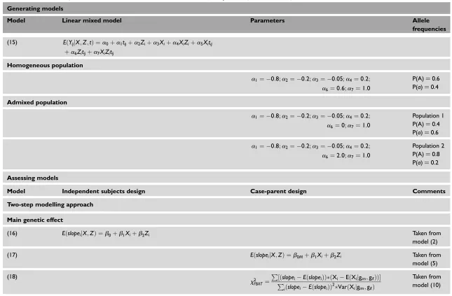
Table S1. List of models used in the simulation process. The column model refers to the number that identifies each model in the paper.Xiis a fixed variable that translates

an offspring genotype to a numeric value;Ziis an observed environmental covariate, either continuous or dichotomous;gim,gifare the parental genotypes (mother and father,

respectively);E(Xijgim,gif) is calculated under segregation and independent assortment assumptions using Mendel’s law;M¼1, 2,. . .,6 are the six possible mating types;

i¼1;2;3;. . .;nsubjects;j¼1;2;3;. . .;mmeasurement occasions into the subject;tijis the repeated ozone exposure variable.

Generating models

Model Linear mixed model Parameters Allele

frequencies

(15) EðYijjX;Z;tÞ ¼a0þa1tijþa2Ziþa3Xiþa4XiZiþa5Xitij

þa₆Zitijþa7XiZitij

Homogeneous population

a1¼ 0:8;a2¼ 0:2;a3¼ 0:05;a4¼0:2;

a6¼0:6;a7¼1:0

P(A)¼0.6 P(a)¼0.4

Admixed population

a1¼ 0:8;a2¼ 0:2;a3¼ 0:05;a4¼0:2;

a6¼0;a7¼1:0

Population 1 P(A)¼0.4 P(a)¼0.6

a1¼ 0:8;a2¼ 0:2;a3¼ 0:05;a4¼0:2;

a6¼2:0;a7¼1:0

Population 2 P(A)¼0.8 P(a)¼0.2

Assessing models

Model Independent subjects design Case-parent design Comments

Two-step modelling approach

Main genetic effect

(16) EðslopeijX;ZÞ ¼b0þb1Xiþb2Zi Taken from

model (2)

(17) EðslopeijX;ZÞ ¼b0Mþb1Xiþb2Zi Taken from

model (5)

(18)

x2

FBAT ¼

P_ð

slopeiEðslopeiÞÞðXiEðXijgim;gifÞÞ

½

P

iðslopeiEðslopeiÞÞ2VarðXijgim;gifÞ

Taken from model (10)

Continued

PRIMAR

Y

RESE

ARCH

Mor

eno-Ma

cias

et

al.

322

#

H

E

N

R

Y

S

T

E

W

A

R

T

P

U

B

L

IC

A

T

IO

N

S

1479

–

7364.

HUMAN

GENO

MICS

.

V

OL

4.

NO

5.

302

–

326

JUNE

(22)

Table S1. Continued

Generating models

Model Linear mixed model Parameters Allele

frequencies

(21) EðslopeijX;ZÞ ¼b0þb1Xiþb2Ziþb3ZiXi Taken from

model (1)

(22) EðslopeijX;ZÞ ¼b0Mþb1Xiþb2MZiþb3ZiXi Taken from

model (9)

Main genetic effect

(19) EðYijjX;Y;tÞ ¼a0þa1tijþa2Ziþa3Xiþa4XiZi

þa5Xitijþa6Zitij

Taken from model (15) witha₇¼0

(20) EðYijjX;Y;tÞ ¼a0Mþa1Mtijþa2Ziþa3Xiþa4XiZi

þa5Xitijþa6MZitij

Taken from model (13) witha7¼0

(23) EðYijjX;Z;tÞ ¼a0þa1tijþa2Ziþa3Xiþa4XiZiþa5Xitij

þa6Zitijþa7XiZitij

(24) EðYijjX;Y;tÞ ¼a0Mþa1Mtijþa2Ziþa3Xiþa4XiZiþa5Xitij

þa6MZitijþa7XiZitij

Gene

–

envir

onment

inter

action

tes

ts

for

fa

m

ily

stud

ies

with

quantita

tiv

e

phen

otypes

PRIMAR

Y

RESE

ARCH

#

H

E

N

R

Y

S

T

E

W

A

R

T

P

U

B

L

IC

A

T

IO

N

S

1479

–

7364

.

HUMAN

GEN

OMICS

.

V

OL

4.

NO

5.

302

–

326

JUNE

2010