Nadeem Shafique Butt
Department of Social and Preventive Pediatrics, KEMU Lahore
Muhammad Qaiser Shahbaz Department of Mathematics
COMSATS Institute of Information Technology, Lahore, Pakistan
Shahid Kamal
College of Statistical and Actuarial Sciences University of the Punjab, Lahore
Abstract
Almost all available statistical packages are capable of performing Multivariate Analysis of Variance (MANOVA) from raw data. Some of statistical packages have capability to perform independent sample t-test, ANOVA and some other tests of significance on summary data, but you come across not single software that has the capability to perform MANOVA directly on summary data. A STATA programme has been written to perform Multivariate ANOVA on summary data. The programme computes available statistics for Multivariate ANOVA (i.e Willk’s Lembda, Lawley’s-Hotelling trace, Pillae’s trace and Roy’s largest root). The programme is also capable to perform Box–M test for testing equality of covariance matrices on summary data. Example has been given by using the programme on summary data to perform Multivariate ANOVA.
Keywords: ANOVA, MANOVA, Summary data.
1. Introduction
Multivariate ANOVA (MANOVA) has been widely used for comparison of several factors when information on several variables has been collected. The simplest case is One Way MANOVA where levels of single factors are compared on the basis of information of several variables. One simple use of One Way MANOVA is to test the equality of mean vectors of several Multivariate Normal populations having common covariance matrix.
Most of the statistical packages are designed to conduct several test of significance when raw data is available, but in many practical situations only summary information is available (e.g. n s' , X s' ,S D s. ' ,. . . ) from some
According to Larson one has to generate two new columns namely Xj's and
'
n
X sas
2
' ' j j
j X s X s
n
s
= + and Xn's n X= j j−
(
nj−1)
Xj'sAnd after some data manipulation data is ready to perform ANOVA in usual way.
Butt et al (2006) used an alternative method that can be used to perform one way, two way and higher way ANOVA by using summary measures n xj, j and sj
for j=1, 2,..., ,k where n xj, j and sj are, respectively, the size, mean and standard deviation of j–th treatment. In this paper we extend this idea for the Multivariate Analysis of Variance case and have developed a STATA programme that can be used to perform one way MANOVA on summary data.
2. Methodology
The Multivariate ANOVA is a natural extension of the univariate ANOVA. In this technique the observation vectors are available from the multivariate normal populations having common covariance matrices. The task is to compare the mean vectors of these multinormal populations. Extending the idea of univariate study, the multivariate ANOVA can be presented as the Multivariate Linear Model. Specifically, the one way multivariate ANOVA model is given as:
(
)
1, 2,...,; ;
1, 2,...,
ij j ij ij p
j
j k
has N and
i n
= ⎧
= + + ⎨ =
⎩
x μ τ ε ε 0 Σ (2.1)
The hypothesis of interest in the fixed effect one way MANOVA model is generally given as:
(2.2)
Another simple use of the one way MANOVA model is to test the hypothesis:
0: 1 2 k
H μ =μ = ⋅⋅⋅⋅⋅⋅ =μ (2.3)
when independent random samples are available from Np
(
μ Σj;)
.Several test statistics are available in literature that enables us to test the hypothesis given in (2.2) and (2.3). The most popular of these statistics is the one given by Willks (1932). The statistic given by Willks (1932) is the ratio of two generalized variances and is given as:
(
)
(
)
1
0 1
1 2 1 1
1
S
S ms p k
F
p k
⎡ − − + ⎤ − Λ
=⎢ ⎥⋅
− Λ
⎢ ⎥
with
(
)
/ /1 1
; 1 ;
k k
j j j j j
j j
n n n
= =
Λ = = − = −
+
∑
∑
W
W S B x x xx
B W (2.5)
The quantities xj and Sj are the mean vector and covariance matrix for j – th group and x is the combined mean. The statistic given in (2.4) has an exact
( 1 ;) ( 1 2 1)
p k ms p k
F − − − + where:
(
) (
)
(
)
(
)
2 2 2 2 2 1 41 2 ;
1 5
p k
m n p k S
p k
− −
= − − + =
+ − − (2.6)
Another statistic proposed by Hotelling (1951) is based upon the trace of T B−1 and is given as:
(
1)
V =tr T B− ;
(
)
(
)
(
)
1
1 1
1 1 1
n k p a V
F
k p a a V
− − − + + ⎡ ⎤ ⎣ ⎦ = ⎡ − − − + + ⎤ − ⎣ ⎦
;a=min
(
k−1,p)
(2.7)The expression given in (2.7) has: F⎡(k− − − + +1 p 1) a 1 ;⎤ ⎡(n k p− − − + +1) a 1⎤
⎣ ⎦
⎣ ⎦
Pallie’s trace (1955) has proposed yet another statistic based upon the trace of
1
−
W B. This statistic is given as:
(
1)
(
(
)
)
2 2
2 1 / 2 1
; F
2 1 1 / 2 1
U a n k p
U tr
a k p a
− ⎡⎣ − − − + ⎤⎦
= =
⎡ − − − + + ⎤
⎣ ⎦
W B (2.8)
The expression given in (2.8) has:
F
a k⎡ − − +1 p a a n k p⎤; ( − − − +1) 2⎣ ⎦
Roy (1953) built his statistic on the largest root of W B−1
. His statistic is given as:
( )
max i ;
R= λ F3 R n b
(
1)
;b max(
k 1,p)
b− −
= = − (2.9)
i
λ are eigen values of W B−1
;
The expression given in (2.9) has : Fb n b; − −1
The programme also performs the Box (1949) test for equality of covariance matrices by using the statistic:
(
)
(
)
(
)
10
1
; ln 1 ;
k
j j
j
B MC M n k n n k −
=
= = − S −
∑
− S S= − W (2.10)(
)(
)
2
1
2 3 1 1 1
1
6 1 1 1
k
j j
p p
and C
k p = n n k
⎡ ⎤
+ −
= − ⎢ − ⎥
− + ⎢⎣
∑
− − ⎥⎦3. STATA Program
In this section we have given a Stata Mata program named “manovai.ado” that can be used to perform the MANOVA on summary data. The program “manovai.ado” requires four arguments as input, variable of group identification, variable of sample sizes, variable of mean vectors and variables of variance-covariance matrices respectively.
--- manovai.ado
program manovai, rclass version 9 syntax varlist marksample touse
mata: manovai("`varlist'", "`touse'")
end version 9
mata:
function manovai(string scalar varnames, string scalar touse) {
string rowvector vars, rhsvars string scalar lhsvar, samp, gr
real matrix v, b,t, sum, sumb, sumw real scalar count, gn, gm, dt
real colvector m, g, W vars = tokens(varnames)
gr = vars[1] samp = vars[2] lhsvar = vars[3] rhsvars = vars[|4\.|]
st_view(v, ., rhsvars, touse) st_view(m, ., lhsvar, touse)
st_view(s, ., samp, touse) st_view(g, ., gr, touse) info = panelsetup(g,1)
stats=panelstats(info) count = stats[4]
k = stats[1]
sumw = J(count,count,0) sumb = J(count,count,0)
gn = 0
dt = 0
nj = 0
gm = J(count,1,0) for (i=1; i<=rows(info); i++)
v_i = panelsubmatrix(v, i, info) m_i = panelsubmatrix(m,i,info) n_i = panelsubmatrix(s,i,info)
n = mean(n_i)
det = (log(det(v_i)))*(n-1) w_i=(n-1)*v_i
b_i=n*m_i*(m_i)'
gn = gn + n
gm = ((gm + m_i*n)) sumw = sumw + w_i sumb = sumb + b_i
dt = dt + det
nj = nj + 1/(n-1)
}
summ = summ sumb = sumb gm = gm/gn
sumb=sumb - gn*gm*gm' t = sumb + sumw
mm = (gn-1)-(count+k)/2
s = ((count^2*(k-1)^2 - 4)/(count^2+ (k-1)^2 - 5))^0.5 df1 = count*(k-1)
df2 = mm*s - ((count*(k-1))/2)+1 gdf = (k-1)
df = (gn -1) edf= df - gdf W = (k-1,count) w = min(W) d = max(W)
m = (gn-k)*log(det(sumw/(gn-k)))-dt
c = 1- (((2*count^2 + 3*count + 1)/(6*(count+1)*(k-1)))*(nj-1/(gn-k))) q = m*c
df_q= (count*(count+1)*(k-1))/2 PQ = 1- chi2(df_q,q)
Lam = det(sumw)/det(t)
FW = (df2/df1)*(1-Lam^(1/s))/(Lam^(1/s)) PW=1- F(df1,df2,FW)
V= trace(invsym(t)*sumb)
df1_p= w*((abs((k-1)-count)-1)+ w +1) df2_p= w*((gn-k-count-1)+ w + 1)
U = trace(invsym(sumw)*sumb)
FL = (2*(w*(gn-k-count-1)/2+1)*U)/(w^2*((2*(abs(k-1-count)-1)/2)+w+1)) PL = 1- F(df1,df2,FL)
df1_l= w*((abs((k-1)-count)-1)+ w +1) df2_l= w*(gn-k-count-1)+2
r = eigenvalues(invsym(sumw)*sumb) r = Re(r)
R = max(r)
FR = R*((gn-k-d+k-1)/d) PR = 1- F(df1,df2,FR) df1_r= d
df2_r= (gn-k-d+k-1)
}
end
--- manovai.ado
4. Numerical Example
In this section we have given a hypothetical example to demonstrate the usefulness of the program that can be used to perform MANOVA on summary statistics.
Example
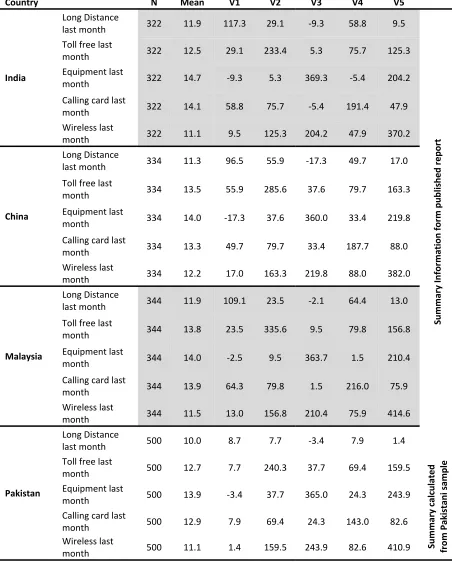
In particular, the telecommunication company has separated the monthly bill into amounts spent on Long distance, Toll free, Equipment, Calling card, and Wireless services, and categorized the customers based upon countries (India, China, Malaysia) and apply MANOVA test to see is there significant difference in monthly billings of these three countries. Suppose the results are published in a report along with summary statistics. Now suppose you wish to compare how monthly billings in Pakistan are different from these three countries.
Table 4.1: Summary data that obtained from published report and calculated from Pakistani sample
Variance ‐ Covariance
Country N Mean V1 V2 V3 V4 V5
India
Long Distance
last month 322 11.9 117.3 29.1 ‐9.3 58.8 9.5
Sum m ary In formation form pu blis he d report
Toll free last
month 322 12.5 29.1 233.4 5.3 75.7 125.3
Equipment last
month 322 14.7 ‐9.3 5.3 369.3 ‐5.4 204.2
Calling card last
month 322 14.1 58.8 75.7 ‐5.4 191.4 47.9
Wireless last
month 322 11.1 9.5 125.3 204.2 47.9 370.2
China
Long Distance
last month 334 11.3 96.5 55.9 ‐17.3 49.7 17.0
Toll free last
month 334 13.5 55.9 285.6 37.6 79.7 163.3
Equipment last
month 334 14.0 ‐17.3 37.6 360.0 33.4 219.8
Calling card last
month 334 13.3 49.7 79.7 33.4 187.7 88.0
Wireless last
month 334 12.2 17.0 163.3 219.8 88.0 382.0
Malaysia
Long Distance
last month 344 11.9 109.1 23.5 ‐2.1 64.4 13.0
Toll free last
month 344 13.8 23.5 335.6 9.5 79.8 156.8
Equipment last
month 344 14.0 ‐2.5 9.5 363.7 1.5 210.4
Calling card last
month 344 13.9 64.3 79.8 1.5 216.0 75.9
Wireless last
month 344 11.5 13.0 156.8 210.4 75.9 414.6
Pakistan
Long Distance
last month 500 10.0 8.7 7.7 ‐3.4 7.9 1.4
Toll free last
month 500 12.7 7.7 240.3 37.7 69.4 159.5
Sum m ary calc ulated from Paki stani sam p le
Equipment last
month 500 13.9 ‐3.4 37.7 365.0 24.3 243.9
Calling card last
month 500 12.9 7.9 69.4 24.3 143.0 82.6
Wireless last
Table given in table 4.1 can be entered directed into Stata data editor in the following manner
References
1. Box, G. E. P. (1949). A general distribution theory for a class of likelihood ratio criteria, Biometrike, 36, 317 – 346.
2. Butt, N. S., Kamal, S., Shahbaz, M. Q. (2006). “ANOVA using summary data: A STATA programe” Pak Jour. Of Stat. and Oper. Res. Vol. 2(1).
3. Hotelling, H. (1951). A generalized T test and measure of multivariate
dispersion, Proceeding of the Second Berkeley Symposium on
Mathematical Statistics and Probability, University of California, Los Angeles and Berkeley, 23 – 41.
4. Pillai, K. C. S. (1955). Some new test criteria in multivariate analysis,
Annals of Mathematical Statistics, 26, 117 – 121.
5. Roy, S. N. (1953). On a heuristic method of test construction and its use in multivariate analysis, Annals of Mathematical Statistics, 24, 220 – 238.
6. Wilks, S. S. (1932). Certain generalizations in the analysis of variance,