Depth image-based plane detection

R E S E A R C H

Open Access

Depth image-based plane detection

Zhi Jin

, Tammam Tillo

, Wenbin Zou

, Xia Li

and Eng Gee Lim

*Correspondence: [email protected]

1_{School of Information Engineering,}

Shenzhen University, Nanhai Ave 3688, 518000 Shenzhen, People’s Republic of China

Full list of author information is available at the end of the article

Abstract

Background: The emerging of depth-camera technology is paving the way for variety of new applications and it is believed that plane detection is one of them. In fact, planes are common in man-made living structures, thus their accurate detection can benefit many visual-based applications. The use of depth data allows detecting planes characterized by complicated pattern and texture, where texture-based plane detection algorithms usually fail. In this paper, we propose a robust Depth

Image-based Plane Detection (DIPD) algorithm. The proposed approach starts from the highest planarity seed patch, and uses the estimated equation of the growing plane and a dynamic threshold function to steer the growing process. Aided with this mechanism, each seed patch can grow to its maximum extent, and then next seed patch starts to grow. This process is iteratively repeated so as to detect all the planes.

Results: Validated by extensive experiments on three datasets, the proposed DIPD algorithm can achieve 81% correct detection ratio which doubles the value compared with the state-of-the-art algorithms. Meanwhile, the runtime of the proposed algorithm is around 4 times of the fastest RANdom SAmple Consensus (RANSAC).

Conclusions: The proposed depth image-based plane detection algorithm can achieve state-of-the-art performance. In terms of applications, it could be used as the pre-processing step for planar object recognition, super-resolution of the intrinsically low resolution Time-of-Flight (ToF) depth images, and variety of other applications.

Keywords: Plane detection, Depth image, Region growing, Dynamic threshold function, ToF depth camera

Background

Man-made indoor and outdoor structures are generally dominated by different shapes of planes. These planes carry orientation and size information of the 3D objects in the scene. Therefore, 3D reconstruction can be simplified by detecting these planes and set-ting up the piecewise planar model of the indoor and outdoor scenes [1–3]. Moreover, plane detection technique has been widely used in robot navigation systems [4] and the computer vision for object recognition [5].

At the early stage of the plane detection technique, texture information is mainly adopted. However, this approach may fail when a plane has inconsistent color or texture. As a remedy to this limitation, depth maps offer one clue and turns out to be effec-tive in texture challenging situations. With the increasing availability of consumer depth cameras, e.g., SwissRanger SR4000 [6] and Microsoft Kinect [7], the depth-based plane

segmentation and plane detection become popular. Since depth map represents the spa-tial information of each point in the scene, the points from the same plane will have similar spatial features, such as gradients and normal vectors. Based on this, Holz et al. [8] implemented the real-time plane detection by extracting three components of the normal vector of each point and clustering the points with similar orientations. As parallel planes have similar normals, all the extracted planes, later on, are refined by their distance to the origin. Although, the depth-based plane detection approaches can be implemented in real-time by checking the points’ normal vectors, they suffer from low accuracy and pre-cision. Moreover, due to the fact that the local normal vector is obtained based on a fixed number of neighboring points, if the number is small (e.g., 2), the normal vector is easily affected by noise points. However, if the number is large, the normal vector for boundary points is inaccurate. For robotic navigation system, the detection speed is more strictly required than its accuracy. Hence, using normal vectors is sufficient, whereas for other applications, for example, the human navigation system for guiding the visually impaired person, the detection accuracy is more important. Therefore, in this work, we will target on the accuracy and robustness of the proposed plane detection algorithm.

To satisfy this requirement, we present an unsupervised plane detection algorithm on consumer Time-of-Flight (ToF) depth camera captured depth maps, named Depth Image-based Plane Detection (DIPD). The proposed DIPD algorithm detects planes by adopting a dynamic seed growing approach. The growing starts from the highest planarity seed patch and is steered by the estimated equation of the current growing plane. Moreover, the estimated equation is refined at each growing stage by taking the newly incorporated pixels into account. The growing process is iteratively carried out until all the planes get detected. More advanced than the previous work [9], in this work, a dynamic thresh-old function which takes both the plane attributes and noise model of depth cameras into account, is proposed to enhance the detection accuracy and robustness. These, later on, have been validated by comprehensive and extensive experiments on three datasets. The proposed plane detection process can be taken as a necessary step for further pla-nar object recognition (floor, walls, table-tops, etc.) [10], indoor scene reconstruction [11] and place recognition [12].

In short summary, the major contributions of this proposed work are as follows: (1) In our algorithm, no RGB information is used and no per-pixel normal vector estimation is required. (2) We proposed a patch-based seed selection approach rather than separated or randomly selected seed points and the plane growing always starts from the seed patch with the largest planarity. This can ensure the growing process starts from a small plane. (3) We novelly proposed a dynamic threshold function in the growing process, which takes both the process and ToF depth camera noise model into account. Therefore, in contrast to existing algorithms, the proposed one can efficiently alleviate over-growing and under-growing problem. (4) Extensive experiments are performed to validate the proposed approach. Our results show a significant performance improvement for the challenging indoor scene on different depth datasets.

Iterative plane fitting methods

fitting model is obtained based on several randomly selected points. This method is effi-cient in detecting large planes and robust to noisy data, however, it tends to over-simplify complex planar structures. For example, the horizontal and vertical planes in a stair-step structure are often detected as one plane aligned with the stair slope. Hence, in order to tackle this problem, RANSAC is usually combined with other detection or refinement methods, such as Minimum Description Length (MDL) [14], and Normal Coherence Checking (NCC-RANSAC) [15].

Hough transform-based methods

The Hough Transform is well-known for parameterized objects detection, typically for detecting lines and circles in 2D datasets [16]. Aiming to extend its usage to 3D space and meanwhile, to reduce its computational cost, numerous variations have been proposed. 3D Hough Transform proposed by Hulik et al. [17] describes each plane by its slope along xandyaxes and the distance to the origin of the coordinate system. Although in contrast to RANSAC, the formulation of Hough Transform-based methods is sound, the voting process makes them suffer from high computational cost in finding the parameters of one fitting model, especially when the input data is large or the accumulator is sensi-tive. Randomized Hough Transform (RHT) [18] as an alternative approach avoids high computational cost of the voting process. Instead, for every pixel, it calculates the model parameters in a probabilistic way. Dube et al. [19] proposed a plane detection method by applying RHT on Kinect generated depth map which allows detecting the planes in real time. For a more comprehensive review of Hough-based methods on plane detection, please refer to [18].

Region-growing-based methods

Scan line grouping methods

For segmenting 3D laser range scans, scan line grouping methods are widely adopted. The basic idea behind this method is that 3D planes in a 3D scan are observed as 2D straight lines and if two straight lines cut one another, they lie in one plane [25]. As a derivative of region growing methods, the growing primitives are scan lines instead of individual pixels. In this regard, scan line grouping increases computational efficiency by first detecting lines in planar cuts and then merging neighboring line segments to regions. Hemmat et al. [26] realized the plane detection in three steps. Firstly, all 3D edges in a depth image were searched and the lines between these edges were found. Then, all the points on each pair of intersecting lines were merged into a plane and finally, filtering enhancements were applied to improve the segmentation accuracy.

Methods

More advanced than the previous work [9], the working principles of seed genera-tion and region growing are reformulated using clear mathematic expressions in this section, respectively. Moreover, a novel dynamic growing threshold function is proposed to increase the detection accuracy and robustness by considering the noise model of consumer depth cameras and the characteristics of the region growing process.

Valid seed patches generation

Seed selection is a crucial step in region-growing methods. Indeed, the results of the detection are highly dependent on the initial seeds from which regions are expanded. Since some holes or anomalous points may exist in the hardware generated depth maps, without checking the points’ validation, randomly picking up the seed points can easily lead to the failure of the model fitting, which also increases the computational cost for determining the optimal fitting plane. Moreover, by neglecting the neighbor relationships, randomly selected seed points have high probability from different planes, which easily cause the failure of finding the best fitting plane. Hence, in order to ensure that the grow-ing process is established on reliable seed points, a slidgrow-ingL×Lsquare window moves in raster-scan fashion by one pixel each time on the whole depth map, and at each position, all the involved points will be checked. The patch, which is free from holes, is regarded as onevalid seed patchand denoted asψiwithibeing the seed generation index. The perfor-mance differences caused by different seed patch sizes are discussed in the experimental section.

In the 3D space, a plane can be represented by its normal vectornˆ and the distance from the 3D space origind. For an arbitrary pointp=(x,y,z)on this plane, the Hessian form of the plane can be written asnˆ·p+d=0 and the operation “·” stands for the dot-product of two vectors. By applying the Linear Least Squares (LLS) plane fitting approach to each valid seed patch, the best fitting planesi can be found to represent the seed patch. The distance (or fitting error) between the best fitting plane and its pointpcan be evaluated as:

e(p)=nˆi·p+di (1)

δi=

1

|P|

∀p∈P

ˆ

ni·p+di 2

=

1

|P|

∀p∈P

e2_{(p) (2)}

The root mean square fitting error indicates the planarity of the seed patch. Thus less fitting error means higher planarity. These values later on are used to sort all the valid seed patches.

Region growing process

This subsection explains the iterative growing process of a plane starting from a seed patch. First of all, some notations that will be used throughout the article need to be intro-duced. The indexjis used as a superscript to indicate the iteration index of the growing process. For example, a planeSiatj-th stage of the growing process will be represented bySj_iorSj_i f_ij,δj_iwheref_ijandδj_iare the estimated equation and root mean square fitting error of the plane, respectively. Once the plane grows to its final stage, it will be repre-sented hereinafter bySiorSi f_iki,δk_ii

, wherekirepresents the index of the last growing

stage of this plane andfki

i is the final estimated plane equation.

Different from RANSAC-based methods [13,15] whose seeds are selected randomly, in the proposed growing stage, all the previously valid seed patches will be initially arranged in ascending order of their fitting error in a growing seed list 1, thus

1 = {∀ψn,ψm∈1:δn≤δm;n<m}. For the seed patches having the same fitting error, the earlier generated one appears earlier in the seed list. The first seed patch appear-ing in the list will be used to initiate the first plane. Once the first plane reaches its maximum extent, it stops to grow and the seed list is updated to2by eliminating all the

seed patches that get englobed in the detected plane. This updating process will be car-ried out at the end of the growing process of each plane to generate a new growing seed listi+1 = {∀ψm∈i:ψm∈/Si}whereiis the detected plane index. This can ensure that only the valid seed patch, which is non-incorporated in previously detected planes and ranked as the first one in the new growing seed list, will be used in the subsequent detection of other planes.

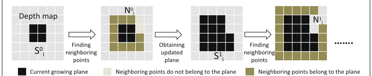
At the beginning of the growing process of planeSi, its initial representation equation is merely defined by its seed patch. Thus,S_i0f_i0,δ_i0 = sm, withsm being the best fit-ting plane of the first seed patch ini. Referring to Fig.1which shows an example of the first two growing stages (i.e.,j = 1 andj = 2) of the planeSi. At the first grow-ing stage, all the 8-connected neighborgrow-ing points N_i0 [27] of seed patch are checked. When no holes are found, meanwhile, no points belong to any previously detected plane, N_i0 = {p:p∈/Sm,m<i}, the neighboring points are substituted into plane equation

f_i0separately to get the corresponding fitting error by (1). If the fitting error is above a threshold,T, the corresponding neighboring point is regarded as an outlier to this current growing plane. Otherwise, this point is incorporated into this plane. After the first grow-ing stage, the plane equationf_i0will be refined tof_i1using the LLS plane fitting approach over the whole involved points andδ_i0is updated toδ_i1by (2). The similar process will be repeated for the rest growing stages and it could be summarized by:

S_ij+1\Sj_i=∀p ∈N_ij:e(p)≤T(d,j) (3)

whereT(d,j) is the threshold which is a function of depth valuedand the number of growthj.

Since the key to region growing-based plane detection is to accurately distinguish the inliers and outliers of the current growing plane, the judgement which is conducted by the distance thresholdTplays an important role. For most of the region growing-based meth-ods, fixed threshold is used in growing process. However, this easily causes over-growing (the threshold is set large) or under-growing (the threshold is set small). Therefore, several works begin to take the depth camera noise model into the design of threshold function.

As suggested in [28] that for consumer depth camera the noise in range sensors usually increases quadratically with the measured distance, Holz et al. [21], Nguyen et al. [29] and Smisek et al. [30] adopted a simple quadratic polynomial as a function of distance to determine the threshold.

T(d)=αd2+βd+γ (4)

whereα,β andγ are three constants but with different values in the three works due to different assumptions. Holzer et al. [31] and Deng et al.[10] in their works provided a noise model solely based on the quantization effect induced by the measurement principle of depth sensors. Therefore, the corresponding threshold is only proportional to the square of depth.

T(d)=κd2 (5)

whereκ is a constant. By conducting a set of experiments to evaluate the influence of the threshold function for plane detection, it is found that although the final detection performance does not considerably deviate for the different threshold functions, the best results can be achieved with a combination of the quadratic polynomial models and the depth square models [22]:

T(d)=

αd2+βd+γ ; d≤d0

κd2 ; d>d0

(6)

whered0is the depth value that makesαd2+βd+γ =κd2.

their surface materials, they may also contain large noise. Therefore, a small threshold eas-ily causes under-growing in this case. Secondly, the planes far from the camera but with small size are easily over-growing due to the large threshold. Thirdly, if the growing plane is perpendicular to the camera plane, the threshold becomes a fixed number. However, with more and more points get involved in the growing plane, noise is also accumulated. In this case, the perpendicular plane trends to be under-growing.

In order to overcome above mentioned weaknesses, we propose a threshold function that takes both the noise model and the plane size into consideration. Moreover, inspired by (6), the proposed threshold function is in a combination format.

T(d,j)= τ

1−e−j/λ2 _{; j≤} H×W κ2

αd2×τ1−e−j/λ2 ; j> H×_κ2W (7)

whereτis the maximum allowed “roughness” of the plane,λdecides the changing speed of the threshold,H andW represent the size of the depth map andα andκ are two constants. Hence, for each plane,T(d,j)is initialized byj=1 and the maximum threshold value is either determined byjifj≤ H×_κ2W or by the distance of points being checked. The parameterτcan be tuned to suit different object reflectivities and to make the detection of planes more robust to depth map noise. Meanwhile, the parameterλallows to set the increasing speed of the threshold at initial growing stages for different situations.

This kind of elaborate design can well tackle the mentioned problems met by noise-model-based thresholds in literature. Since the number of growth can indirectly indicate the plane size, within a certain range the thresholdT(d,j)is dynamically updated only based on the plane size. Specifically, when the growing plane is in its small or medium size, the threshold negative exponentially increases with the growing number. It can lead to two benefits. Firstly, by considering the plane size, even if for the small and far planes, it could avoid the over-growing problem caused by a large threshold. Secondly, by consid-ering the noise accumulation in growing process, even if the growing plane is parallel to the camera plane, the threshold is not a fixed number. With continuously growing, both plane size and the point distance have joint effects on the threshold. However, the impact of plane size decreases while the growth number increases. Finally, the point distance will be predominant to determine the threshold. Hence, for large planes, the threshold follows the camera noise model that further planes suffer from more noise than the closer ones and consequently, the corresponding threshold should be larger. In addition, the prob-lems caused by planes with rough surfaces can be well handled by setting the maximum allowed roughnessτto a relatively large value.

By adopting the proposed threshold function, the growing process for the planeSiwill be iteratively repeated until one of the following termination conditions is met: (a) the neighboring setN_ijis empty, (b) no point inN_ijfits well into the current growing plane. These two conditions indicate that thei-th plane grows to its maximum extent. As pre-viously described at the end of the growing process of thei-th plane, a new growing seed list,i+1, will be generated and a new round of growing process will be initiated by the

Computational complexity analysis

In order to clearly analyze the computational complexity of the proposed DIPD algorithm, we decompose the whole algorithm into three main processes which are seed patches generation, region growing and refinement. For a ToF depth camera generated depth map, its size isW×Hand containsn = W×H points. If the size of the sliding win-dow that used to generate seed patch isL×Land each time the sliding window only moves one pixel, the number of generated seed patch ism = (W−L+1)(H−L+1). Since the optimal plane fitting for each seed patch needs constant time, the computa-tional complexity for seed patches generation in total isO(m). However, this complexity could be reduced by enlarging the sliding window step size, so that the seed patches are generated right next to each other. In this case, the number of seed patches can drop tom= W_L×2H. Due to the adoption of point-based growing approach, the complexity of region growing processes isO(nlogn). The complexityO(m)compared withO(nlogn) can be neglected, and consequently, the overall computational complexity of the pro-posed DIPD algorithm is O(nlogn). Therefore, the proposed approach can increase the accuracy and robustness of plane detection without increasing the computational complexity.

Results

The proposed plane detection approach is validated through extensive experiments on a number of depth maps. To this end, we perform experiments on three types of depth which are generated by ToF depth camera SwissRanger SR4000, a struc-tured light depth camera and computer graphics, respectively. All the types of depth have the ground truth for objective assessment. Although in this work the proposed plane detection algorithm is targeted at ToF camera generated depths which have higher accuracy than the structured light camera generated ones, by testing on other types of depths, the robustness of the proposed algorithm can be validated. In this section, we first briefly introduce each of the adopted depth datasets. Then we evalu-ate the proposed approach on these depths and present both subjective and objective experimental results along with a comparison with the state-of-the-art approaches. Finally, the runtime analysis with respect to well acknowledged RANSCA approach is discussed.

Testing images

Fig. 2The test CG figure. The 3D saw-tooth structure, each “tooth” has different height

Evaluation of the proposed DIPD approach

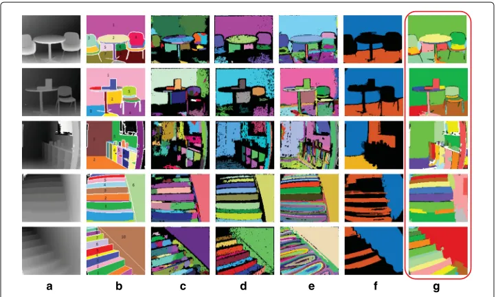
In this subsection, the proposed approach, two state-of-the-art growing-based approaches ([23, 24]) and two RANSAC-based approaches ([10, 33]) are tested on five indoor scenes shown in Fig.4. The depth map and associated ground truth are shown in the first and second column in this figure, respectively. The rest five images are the testing results of CORG method [23], RPCA-based hybrid method [24], CC-RANSAC method [10,33] method and the proposed DIPD method, respectively. In ground truth images, all edges are in white and “uncertain” regions are in black. Whereas, in result images, the black areas or points represent undetected parts. From Fig.4we can observe that these five indoor scenes have various levels of depth complexity. For example,Scene 1(the first row) has a table and wall with uniform textures. Being more complex thanScene 1,

a b c d e f g

Fig. 4Detection comparison. Detection comparison of the proposed DPSD method and the state-of-the-art methods. For each row from left to right is:adepth map of the indoor scene,bcorresponding ground truth, testing result ofcCORG [23],dRPCA [24],eCC-RANSAC [33],fDeng et al. [10] andgthe proposed method (in the red bounding box)

Scene 2has some books on the table and a different kind of chair. The aim of this kind of arrangement is to assess the ability of the proposed DIPD method to distinguish dif-ferent planes forming complicated objects. Then,Scene 3is a more challenging scenario, due to the presence of many small objects, transparent glass and complex combinations of vertical and horizontal planes. Finally,Scene 4andScene 5are the front and side view of a stair-step structure. The stairs scene is known to be challenging for the RANSAC and growing-based plane detection methods.

Fig. 5Two typical cases of over-growing. lateral-OG

obtained in Scene 5 that the parallel vertical stairs is detected as one plane. The threshold updating mechanism in the proposed method allows refining the estimated equations of the detected planes, this can correctly detect curved surfaces with limited curvature, for example, the top-board side surface of the table inScene 1andScene 2. However, for the chairs’ bases inScene 1with large curvature, they will be still detected as the combination of multiple planes rather than one curved surface.

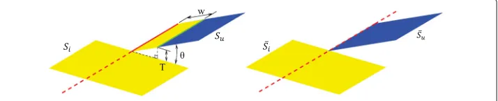
Failure cases analysis: Although the proposed method can correctly detect most of the planes in the scenes, there are still some cases, e.g., intersected planes may make it fail. Refer to Fig.4Scene 5, due to the intersection between the horizontal stair planes and the wall surface, the horizontal stair planes over-grow into the wall surface and cause the later become under-growing. Since during the growing process one plane firstly reaches the intersection line (the red line in Figs.5and6), if the fitting errors of the neighboring points of this intersection line are smaller than the current threshold, the current growing plane will wrongly intrude into its intersecting plane. There are two kinds of growing: over-growing along the lateral side of the intersection line (shown in Fig.5) and over-growing along the intersection line (shown in Fig.6). In the case of Scene 5, the over-growing is lateral over-growing. Another failure case is the under-growing of the wall surface in Scene 4. This is caused by the geometric distortion of the depth map. Although, the pro-posed plane detection algorithm can correctly detect the planes with limited curvature, due to the geometric distortion the wall surface close to the lens part suffers from a large curvature, which causes the failure of the proposed algorithm. Hence, these failure cases limit the accuracy and robustness of the proposed algorithm. Further post-processing is required to overcome the over-growing and under-growing problem.

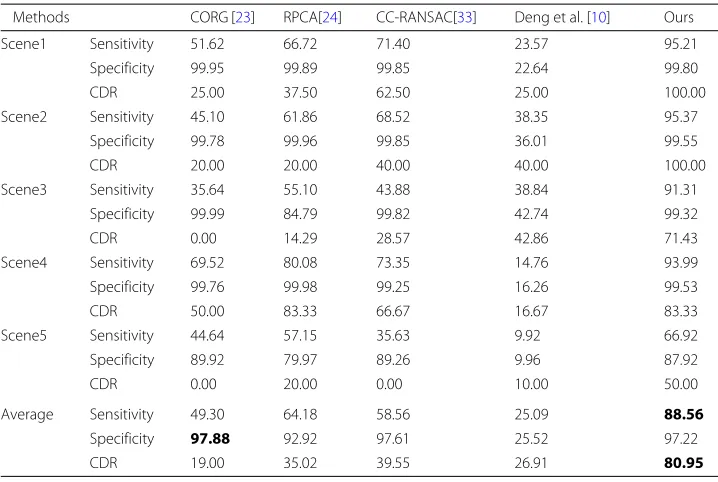
The objective assessment of the proposed method is shown in Table1using the Receiver Operating Characteristic (ROC) of labeled planes in ground truth. In this table, detection sensitivity can be expressed assensitivity=TP/(TP+FN); specificity can be expressed asspecificity=TN/(TN+FP); Correct Detection Ratio (CDR) counts for in each scene how many labeled planes are correctly detected, and one plane that has over 80% over-lap with the ground truth is regarded as a correctly detected plane. “TP” (True Positive)

Table 1The ROC results on ToF camera generated depth maps (all results are in percentage)

Methods CORG [23] RPCA[24] CC-RANSAC[33] Deng et al. [10] Ours

Scene1 Sensitivity 51.62 66.72 71.40 23.57 95.21

Specificity 99.95 99.89 99.85 22.64 99.80

CDR 25.00 37.50 62.50 25.00 100.00

Scene2 Sensitivity 45.10 61.86 68.52 38.35 95.37

Specificity 99.78 99.96 99.85 36.01 99.55

CDR 20.00 20.00 40.00 40.00 100.00

Scene3 Sensitivity 35.64 55.10 43.88 38.84 91.31

Specificity 99.99 84.79 99.82 42.74 99.32

CDR 0.00 14.29 28.57 42.86 71.43

Scene4 Sensitivity 69.52 80.08 73.35 14.76 93.99

Specificity 99.76 99.98 99.25 16.26 99.53

CDR 50.00 83.33 66.67 16.67 83.33

Scene5 Sensitivity 44.64 57.15 35.63 9.92 66.92

Specificity 89.92 79.97 89.26 9.96 87.92

CDR 0.00 20.00 0.00 10.00 50.00

Average Sensitivity 49.30 64.18 58.56 25.09 88.56

Specificity 97.88 92.92 97.61 25.52 97.22

CDR 19.00 35.02 39.55 26.91 80.95

The best results are marked in bold

counts the points that have been successfully detected as inliers of the plane and “TN” (True Negative) counts the non-belonging points that have been successfully detected as outliers of the plane. Whereas, “FN” (False Negative) and “FP” (False Positive) counts the points which were wrongly classified as not belonging and belonging to the plane, respec-tively. The average values of detection sensitivity, specificity and CDR are also reported in Table1. From Table1, the proposed method always has the highest sensitivity and CDR than the benchmark methods. However, in terms of specificity, the proposed method is slightly weaker than PRCA and CORG methods. This means our method has a slight trend of over-growing, nevertheless, the benchmark methods have a clear trend of either under-growing or over-growing. Since the missing detection of areas has huge negative impacts on both the sensitivity and specificity values, the undetected areas and points bring down these values of RPCA and [11] methods. While, the under-growing prob-lem and over-growing probprob-lem bring down the sensitivity value of CORG method and the specificity value of CC-RANSAC method, respectively. For the details of objective assessment of each plane, please refer to the project website.

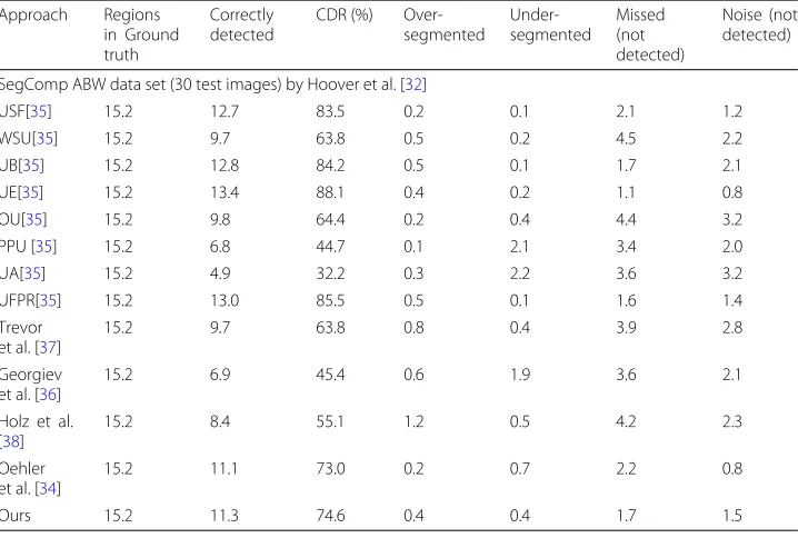
Table 2Comparison with other plane segmentation approaches on the SegComp ABW dataset Approach Regions in Ground truth Correctly detected

CDR (%)

Over-segmented Under-segmented Missed (not detected) Noise (not detected)

SegComp ABW data set (30 test images) by Hoover et al. [32]

USF[35] 15.2 12.7 83.5 0.2 0.1 2.1 1.2

WSU[35] 15.2 9.7 63.8 0.5 0.2 4.5 2.2

UB[35] 15.2 12.8 84.2 0.5 0.1 1.7 2.1

UE[35] 15.2 13.4 88.1 0.4 0.2 1.1 0.8

OU[35] 15.2 9.8 64.4 0.2 0.4 4.4 3.2

PPU [35] 15.2 6.8 44.7 0.1 2.1 3.4 2.0

UA[35] 15.2 4.9 32.2 0.3 2.2 3.6 3.2

UFPR[35] 15.2 13.0 85.5 0.5 0.1 1.6 1.4

Trevor et al. [37]

15.2 9.7 63.8 0.8 0.4 3.9 2.8

Georgiev et al. [36]

15.2 6.9 45.4 0.6 1.9 3.6 2.1

Holz et al. [38]

15.2 8.4 55.1 1.2 0.5 4.2 2.3

Oehler et al. [34]

15.2 11.1 73.0 0.2 0.7 2.2 0.8

Ours 15.2 11.3 74.6 0.4 0.4 1.7 1.5

the UB algorithm uses a novel approach that exploits the scan line structure of the image. The parameters in these three methods are obtained by training other range images in ABW databset, hence, they can obtain good segmentation results. In UFPR [35], there are 7 parameters needs to determine for each dataset. One problem faced by this approach is that the locally estimated normal vectors are very imprecise when calculated near object vertices or over small, narrow regions. Hence, it easily leads to miss detection and under-segmentation in these regions. The approach of Georgiev et al. [36] considerably has the trend to over-grow planes meeting at obtuse angles, while, the approach of Trevor et al. [37] is weak at detecting smaller planar patches. The approach of Holz et al. [38] suffers from inconsistent normal orientations in this dataset and tends to over-segment the range images. Since only point normal vector at different resolution was used in clustering plane elements in [34], it suffers in the noisy data.

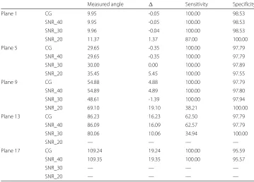
To validate the detection accuracy and robustness of the proposed DIPD method, we test the method on a computer generated depth map (Fig.2). By ordering the 18 planes in Figs.2and 3from left to right, the corresponding outcomes of measured angle, sen-sitivity and specificity for Plane 1, 5, 7, 13 and 17 are listed in Table3. In the table, “” indicates the angle difference between measure tooth angle and ground truth value, “CG” represents the original computer generated depth map. The value following “SNR” repre-sents the noise level and larger number reprerepre-sents less noise contained. The ground truth angles for Plane 1, 5, 7, 13, 17 are 10◦, 30◦, 50◦, 70◦and 90◦, respectively. The equation arccos nˆki

i · ˆn ku

u

is used to measure the angle of a tooth wherenˆki

i andnˆ ku

Table 3Plane detection performance against different levels of Gaussian noise in terms of “Measured angle”(in degree), “Sensitivity”(in percentage) and “Specificity”(in percentage)

Measured angle Sensitivity Specificity

Plane 1 CG 9.95 -0.05 100.00 98.53

SNR_40 9.95 -0.05 100.00 98.53

SNR_30 9.96 -0.04 100.00 98.53

SNR_20 11.37 1.37 87.00 100.00

Plane 5 CG 29.65 -0.35 100.00 97.79

SNR_40 29.65 -0.35 100.00 97.79

SNR_30 30.00 0.00 100.00 97.89

SNR_20 35.45 5.45 100.00 97.55

Plane 9 CG 54.88 4.88 100.00 97.79

SNR_40 54.89 4.89 100.00 97.80

SNR_30 48.61 -1.39 100.00 97.94

SNR_20 69.10 19.10 38.21 100.00

Plane 13 CG 86.23 16.23 62.50 97.79

SNR_40 86.09 16.09 62.57 97.79

SNR_30 80.06 10.06 34.94 100.00

SNR_20 — — — —

Plane 17 CG 109.24 19.24 100.00 95.59

SNR_40 109.35 19.35 100.00 95.57

SNR_30 — — — —

SNR_20 — — — —

specificity. For specificity, lower the value is, severer the over-growing problem is. Hence, the added noise stops the plane to over-grow to some extent and increase the detection accuracy. Compared with sensitivity, the specificity maintains good performance regard-less of the noise, which means the proposed method is better at distinguishing the outliers than the inliers.

Runtime analysis

Table 4Runtime (in seconds) comparison between the proposed algorithm and RANSAC

Methods Total_Time Sensitivity Specificity CDR

Scene1 RANSAC 5.3 49.41 71.66 25.00

Proposed 18.4 95.00 99.78 100.00

Scene2 RANSAC 4.3 57.04 73.60 60.00

Proposed 14.7 95.57 99.42 100.00

Scene3 RANSAC 9.9 36.62 54.75 14.29

Proposed 16.7 59.62 70.51 57.14

Scene4 RANSAC 2.6 29.97 59.94 0.00

Proposed 26.5 78.95 98.71 66.67

Scene5 RANSAC 2.3 27.46 36.17 20.00

Proposed 16.8 49.79 78.00 40.00

Average RANSAC 4.9 40.10 59.22 23.86

Proposed 18.6 75.78 89.28 72.76

with respect to sensitivity and CDR, the performance of our algorithm is still better than that of CORG, RPCA and CC-RANSAC even a large seed size is adopted. It is important to note that when design the whole DIPD algorithm, detection accuracy and the code flex-ibility and re-usability are predominant with respect to the speed, hence, with the gain in performance of the proposed algorithm, it does not sacrifice much more time.

Discussion

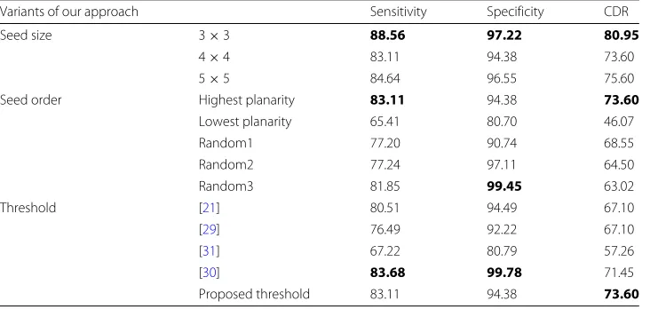
In this section, we discuss the effects of different components in the proposed DIPD on the final performance. Table5summarizes the results achieved on the consumer depth camera generated depth dataset when different components are replaced or removed from the final framework.

In Table5, the effects of different seed sizes are tested first. By comparing the detection results obtained from different seed patch sizes, it can be noticed that employing smaller seed patch initially can achieve more accurate detection result and this will be more supe-rior for complex scenes (e.g. Scene3). In the same scene, it easily causes over-growing by adopting large seed size. Due to the superior performance of using small seed patch size,

Table 5Component analysis on ToF depth camera dataset

Variants of our approach Sensitivity Specificity CDR

Seed size 3_×3 88.56 97.22 80.95

4×4 83.11 94.38 73.60

5×5 84.64 96.55 75.60

Seed order Highest planarity 83.11 94.38 73.60

Lowest planarity 65.41 80.70 46.07

Random1 77.20 90.74 68.55

Random2 77.24 97.11 64.50

Random3 81.85 99.45 63.02

Threshold [21] 80.51 94.49 67.10

[29] 76.49 92.22 67.10

[31] 67.22 80.79 57.26

[30] 83.68 99.78 71.45

Proposed threshold 83.11 94.38 73.60

in our experiment, all the datasets adopt 3×3 seed patch. In terms of different grow-ing seed orders, the plane grows from the seed with the highest planarity gives the best performance than the other two growing orders which is as expected. Since the growth starts from the seed with highest planarity, through each time the plane fitness checking, it has the trend to maintain this planarity during the following growing. On the contrary, if the growth starts from the seed with the lowest planarity, which means it grows from an unperfect fitting plane. Therefore, the fitness error accumulates after each iteration. It is easy to result in under-growing and the growing process becomes sensitive to the depth noise. For each growing starts from randomly selected seed, its performance, as expected, is between the two situations mentioned before. Moreover, since the growing seed patch is randomly selected, it can not guarantee the stableness of plane detection performance. Compared with different threshold functions, we find that the threshold in [31] increases the fastest along with depth values which makes it easily face over-growing problem, so that its detection performance is the worst. Although the threshold function in [30] has highest values in sensitivity and specificity, the proposed threshold function can lead to the highest CDR which means the proposed method can have more planes correctly detected.

Conclusions

In this paper, we proposed a dynamic seed growing mechanism to detect indoor planes using depth maps. The growing starts from the most planar seed patch and grows to its largest extent. Then, next unincorporated most planar seed patch is used, until all the planes are detected. A dynamic threshold function which takes both the plane attributes and noise model of depth cameras into account is adopted in the growing process. The performance of the proposed method has been assessed by comparing with other state-of-the-art methods on the typical indoor scenes and public dataset. The reported results indicate the proposed Depth Image-based Plane Detection (DIPD) method can detect planes with high sensitivity and are robust with respect to various indoor scenes, the chosen parameters and depth noise. As for future work, we aim to exploit the proposed approach for more applications, e.g., depth map up-sampling and depth map coding.

Acknowledgements

The author would like to thank Xiangfei Qian and Prof. Cang Ye from the Department of Systems Engineering, University of Arkansas for their helpful technical support.

Funding

This work is supported by the NSFC Project under Grant 61771321, Grant 61701313, and Grant 61472257, in part by the Natural Science Foundation of Shenzhen under Grant KQJSCX20170327151357330, Grant JCYJ20170818091621856, Grant JCYJ20160307154003475, Grant JCYJ20160506172651253 and Grant JCYJ20170302145906843, in part by the Interdisciplinary Innovation Team of Shenzhen University, and in part by the Natural Science Foundation of SZU under Grant 827-000152.

Availability of data and materials

All the testing data and source code for DIPD algorithm are available in the GitHub repositoryhttps://github.com/jzrita/ DIPD_Project/tree/master/DIPD_test_imagesfor research purpose only.

Authors’ contributions

Ethics approval and consent to participate Not applicable.

Consent for publication Not applicable.

Competing interests

The authors declare that they have no competing interests.

Publisher’s Note

Springer Nature remains neutral with regard to jurisdictional claims in published maps and institutional affiliations.

Author details

1_{School of Information Engineering, Shenzhen University, Nanhai Ave 3688, 518000 Shenzhen, People’s Republic of China.} 2_{The Faculty of Computer Science, Libera Universit di Bolzano-Bozen, Bozen-Bolzano, Italy.}3_{Department of Electrical and}

Electronic engineering, Xi’an Jiaotong-Liverpool University, 111 Ren’ai Road, 215123 Suzhou, People’s Republic of China.

Received: 2 July 2018 Accepted: 26 September 2018

References

1. Cohen A, Schnberger JL, Speciale P, Sattler T. Indoor-outdoor 3d reconstruction alignment. In: European Conference on Computer Vision (ECCV), vol. 9907. Cham: Springer; 2016.

2. Zhang Y, Xu W, Tong Y, Zhou K. Online structure analysis for real-time indoor scene reconstruction. ACM Trans Graph. 2015;34(5):159–115913.

3. Francis E, Jörg S, Bastian L. Joint Object Pose Estimation and Shape Reconstruction in Urban Street Scenes Using 3D Shape Priors. Cham: Springer; 2016, pp. 219–30.

4. Lu Y, Song D. Visual navigation using heterogeneous landmarks and unsupervised geometric constraints. IEEE Trans Robot. 2015;31(3):736–49.

5. Gupta S, Arbelaez P, Girshick R, Malik J. Indoor scene understanding with rgb-d images: Bottom-up segmentation, object detection and semantic segmentation. Int J Comput Vision. 2015;112(2):133–49.

6. http://hptg.com/industrial/(accessed: 15 June 2018).internest. 2014.

7. https://developer.microsoft.com/en-us/windows/kinect(accessed: 15 June 2018).internest. 2014.

8. Holz D, Holzer S, Rusu RB, Behnke S. Real-time plane segmentation using rgb-d cameras. In: In Robot Soccer World Cup. Berlin Heidelberg: Springer; 2011. p. 306–17.

9. Jin Z, Tillo T, Cheng F. Depth-map driven planar surfaces detection. In: Visual Communications and Image Processing Conference, IEEE. Valletta: IEEE; 2014. p. 514–7.

10. Deng Z, Todorovic S, Latecki LJ. Unsupervised object region proposals for rgb-d indoor scenes. Comput Vision Image Underst. 2017;154:127–36.

11. H.Kim HX, Max N. Piecewise planar scene reconstruction and optimization for multi-view stereo. In: Computer Vision(ACCV), 11th Asian Conference on Computer Vision, Daejeon, Korea, November 5-9, 2012, Revised Selected Papers, Part IV. Berlin Heidelberg: Springer; 2013. p. 191–204.

12. Fernández-Moral E, Mayol-Cuevas W, Arévalo V, González-Jiménez J. Fast place recognition with plane-based maps. In: Robotics and Automation (ICRA), IEEE International Conference On. Karlsruhe: IEEE; 2013. p. 2719–24. 13. Fischler MA, Bolles RC. Random sample consensus: A paradigm for model fitting with applications to image analysis

and automated cartography. Commun ACM. 1981;24(6):381–95.https://doi.org/10.1145/358669.358692. 14. Yang MY, Förstner W. Plane detection in point cloud data. In: Proceedings of the 2nd Int Conf on Machine Control

Guidance, Bonn. Bonn: a technical report published by the University of Bonn; 2010. p. 95–104.

15. Qian X, Ye C. Ncc-ransac: A fast plane extraction method for 3-d range data segmentation. IEEE Trans Cybern. 2014;44(12):2771–2783.

16. Hough PVC. Method and means for recognizing complex patterns. U.S. Atomic Energy Commission DTIE; NSA-17-008572, US 3069654, United States. 1962.

17. Hulik R, Spanel M, Smrz P, Materna Z. Continuous plane detection in point-cloud data based on 3d hough transform. J Vis Commun Image Represent. 2014;25(1):86–97.https://doi.org/10.1016/j.jvcir.2013.04.001. Visual Understanding and Applications with RGB-D Cameras.

18. Borrmann D, Elseberg J, Lingemann K, Nüchter A. The 3d hough transform for plane detection in point clouds: A review and a new accumulator design. 3D Res. 2011;2(2):1–13.

19. Dube D, Zell A. Real-time plane extraction from depth images with the randomized hough transform. In: Computer Vision Workshops (ICCV Workshops), IEEE International Conference On. Barcelona Spain: IEEE; 2011. p. 1084–91. 20. Pathak K, Birk A, Vaskevicius N, Poppinga J. Fast registration based on noisy planes with unknown correspondences

for 3-d mapping. Robot IEEE Trans. 2010;26(3):424–41.https://doi.org/10.1109/TRO.2010.2042989.

21. Holz D, Behnke S. Fast range image segmentation and smoothing using approximate surface reconstruction and region growing. In: Proceedings of the Internatinal Conforence on Intelligent Autonomous Systems, IAS, Jeju Island, Korea. Jeju Island: IEEE; 2012.

22. Holz D, Behnke S. Approximate triangulation and region growing for efficient segmentation and smoothing of range images. In: Robotics Autonomous Systems 62. Elsevier; 2014. 62(9):1282–93.

23. Xiao J, Adler B, Zhang J, Zhang H. Planar segment based three-dimensional point cloud registration in outdoor environments. J Field Robot. 2013;30(4):552–82.

25. Jiang X, Bunke H. Fast segmentation of range images into planar regions by scan line grouping. Mach Vis Appl. 1994;7(2):115–22.

26. Hemmat HJ, A P, Bondarev E, de With PHN. Fast planar segmentation of depth images. Proc. SPIE. 2015;9399: 93990–939908.

27. Gonzalez RC, Woods RE. Digital Image Processing. Upper Saddle River: Prentice Hall; 2008.

28. Anderson D, Herman H, Kelly A. Experimental characterization of commercial flash ladar devices. In: Proceedings of the International Conference of Sensing and Technology, Palmerston North, New Zealand. Palmerston North: IEEE; 2005.

29. Nguyen CV, Izadi S, Lovell D. Modeling kinect sensor noise for improved 3d reconstruction and tracking. In: Second International Conference on 3D Imaging, Modeling, Processing, Visualization Transmission. Zurich: IEEE; 2012. p. 524–30.

30. Smisek J, Jancosek M, Tomas P. 3D with Kinect. London: Springer; 2013, pp. 3–25.

31. Holzer S, Rusu RB, Dixon M, Gedikli S, Navab N. Real-time surface normal estimation from organized point cloud data using integral images. In: in:Proceedings of the IEEE/RSJ International Conference on Intelligent Robots and Systems, IROS, Vilamoura, Portugal. Vilamoura: IEEE; 2012. p. 2684–9.

32. Hoover A, Jean-Baptiste G, Jiang X, Flynn PJ, Bunke H, Goldgof DB, Bowyer K, Eggert DW, Fitzgibbon A, Fisher RB. An experimental comparison of range image segmentation algorithms. Pattern Anal Mach Intell IEEE Trans. 1996;18(7):673–89.https://doi.org/10.1109/34.506791.

33. Gallo O, Manduchi R, Rafii A. Cc-ransac: Fitting planes in the presence of multiple surfaces in range data. Pattern Recog Lett. 2011;32(3):403–10.https://doi.org/10.1016/j.patrec.2010.10.009.

34. Oehler B, Stueckler J, Welle DJ, Schulz Behnke S. Efficient Multi-resolution Plane Segmentation of 3D Point Clouds. Berlin: Springer; 2011, pp. 145–56.

35. Gotardo PFU, Bellon ORP, Silva L. Range image segmentation by surface extraction using an improved robust estimator. In: IEEE Computer Society Conference on Computer Vision and Pattern Recognition, 2003. Proceedings. Madison: IEEE; 2003. p. 33–8.

36. Georgiev K, Creed RT, Lakaemper R. Fast plane extraction in 3d range data based on line segments. In: IEEE/RSJ International Conference on Intelligent Robots and Systems. San Francisco: IEEE; 2011. p. 3808–15.

37. Trevor AJB, Gedikli S, Rusu RB, Christensen HI. Efficient organized point cloud segmentation with connected components. Karlsruhe: IEEE; 2013.