Rowan University Rowan University
Rowan Digital Works
Rowan Digital Works
Theses and Dissertations
7-29-2015
Level set segmentation using non-negative matrix factorization
Level set segmentation using non-negative matrix factorization
with application to brain MRI
with application to brain MRI
Dimah DeraFollow this and additional works at: https://rdw.rowan.edu/etd Part of the Electrical and Computer Engineering Commons
Let us know how access to this document benefits you -
share your thoughts on our feedback form.
Recommended Citation Recommended Citation
Dera, Dimah, "Level set segmentation using non-negative matrix factorization with application to brain MRI" (2015). Theses and Dissertations. 517.
https://rdw.rowan.edu/etd/517
This Thesis is brought to you for free and open access by Rowan Digital Works. It has been accepted for inclusion in Theses and Dissertations by an authorized administrator of Rowan Digital Works. For more information, please contact [email protected].
LEVEL SET SEGMENTATION USING NON-NEGATIVE MATRIX
FACTORIZATION WITH APPLICATION TO BRAIN MRI
by Dimah Dera
A Thesis Submitted to the
Department of Electrical & Computer Engineering College of Engineering
In partial fulfillment of the requirement For the degree of
Master of Science in Electrical and Computer Engineering at
Rowan University May 15, 2015
Dedications
I would like to dedicate this work to my mother, my father, my aunt and my husband.
Acknowledgments
I would like to thank my advisor and mentor, Dr. Nidhal Bouaynaya for her guidance, illuminating discussions related to this work and beyond, encouragement and moral and financial support in this research. I also would like to extend my gratitude to Dr. Hassan M Fathallah-Shaykh, Dr. Robi Polikar, Dr. Ravi Prakash Ramachandran and Dr. Nasrine Bendjilali for being part of my committee and for their insights and interest in my work. I continue to be extremely grateful to my family who has been my greatest support. This accomplishment is not mine alone. Thank you for sharing my struggles and my victories. Thank you to my friends and colleagues for sharing my pauses and supporting me during my ups and downs.
Abstract
Dimah Dera
LEVEL SET SEGMENTATION USING NON-NEGATIVE MATRIX FACTORIZATION WITH APPLICATION TO BRAIN MRI
2014-2015
Nidhal Bouaynaya, Ph.D.
Master of Science in Electrical & Computer Engineering
We address the problem of image segmentation using a new deformable model based on the level set method (LSM) and non-negative matrix factorization (NMF). We describe the use of NMF to reduce the dimension of large images from thousands of
pixels to a handful of “metapixels” or regions. In addition, the exact number of regions is discovered using the nuclear norm of the NMF factors. The proposed NMF-LSM characterizes the histogram of the image, calculated over the image blocks, as nonnegative combinations of basic histograms computed using NMF ( ≈ �). The matrix W represents the histograms of the image regions, whereas the matrix � provides the spatial clustering of the regions. NMF-LSM takes into account the bias field present particularly in medical images. We define two local clustering criteria in terms of the NMF factors. The first criterion defines a local intensity clustering property based on the matrix by computing the average intensity and standard deviation of every region. The second criterion defines a local spatial clustering using the matrix �. The local clustering is then summed over all regions to give a global criterion of image segmentation. In LSM, these criteria define an energy minimized w.r.t. LSFs and the bias field to achieve the segmentation. The proposed method is validated on synthetic binary and gray-scale images, and then applied to real brain MRI images. NMF-LSM provides a general approach for robust region discovery and segmentation in heterogeneous images.
Table of Contents
Abstract………...v
List of Figures………...viii
List of Tables……… xi
Chapter 1: Introduction……….……..……1
1.1 Motivation, Problem Statement and Background ……….………1
1.2 Research Contributions ……….5
1.3 Organization ………..7
Chapter 2: Literature Review …………..……….………...9
2.1 Mumford-Shah Model [39] …………..………9
2.2 Chan and Vese Model [7] …………..……….…10 2.3 Localized-LSM Model [25] ………10
2.4 Improved LGDF-LSM Model [10] ………11
Chapter 3: Non-Negative Matrix Factorization ………....13
3.1 NMF and its Variants .………...13
3.1.1 Standard-NMF .……….……….13
3.1.2 Sparse-NMF ……….…..15
3.1.3 Probabilistic Non-Negative Matrix Factorization PNMF [4] . …………..15
3.2 NMF as a Clustering Technique ……..………...16
Chapter 4: Deformable Models ………..……...20
4.1 The Parametric Deformable Model (Snake or Active Contour) .………21
4.2 Drawbacks of the Active Contour Model ……….……..22
Table of Contents (continued)
Chapter 5: NMF-Based Level Set Segmentation ……….…....26
5.1 Region Discovery Using NMF ………...26
5.1.1 Estimating the Number of Distinct Regions in the Image ……….…31 5.1.2 Proof of Lemma 1 .……….………33
5.2 Proposed Variational Framework ………...35
5.3 Level Set Formulation and Energy Minimization ………..39
Chapter 6: Simulation Results and Discussion .……….………...45
6.1 Performance Evaluation and Comparison ….……….……47 6.2 Robustness to Contour Initialization ………...47
6.3 Stable Performance for Different Weighting Parameter ……….50
6.4 PNMF-LSM Evaluation for Small Block Sizes ………..51
Chapter 7: Application to Real Brain MRI Images ………..59
7.1 Robustness to Noise .………..60
Chapter 8: Summary and Conclusion ………..…...69
List of Figures
Figure Page
Figure 1. Rank-2 reduction of a DNA microarray of N genes and M samples is
obtained by NMF, A ≈ WH ………17
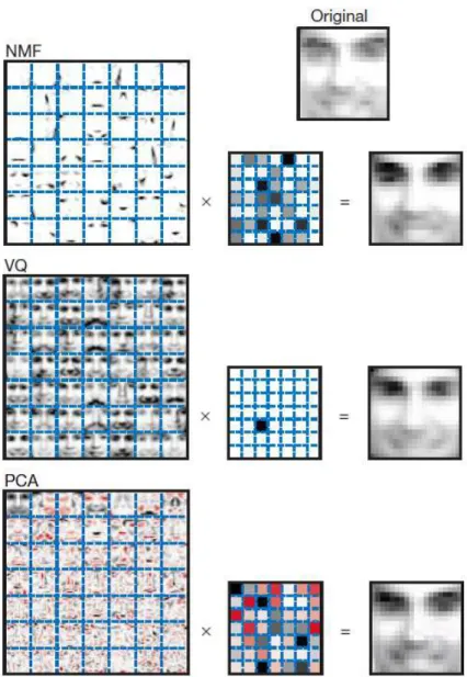
Figure 2. Non-negative matrix factorization (NMF) learns a parts-based representation of faces, whereas vector quantization (VQ) and principal component analysis (PCA) learn holistic representations ……….19 Figure 3. The active contour model fails to handle the topological changes of the moving
fingers [13] ………..23
Figure 4. Building the data matrix and histogram factorization using PNMF …………..28 Figure 5. “ ” and “�” matrices interpretation for a synthetic binary image with
× block size and the entries of � normalized for each column ……....30 Figure 6. A synthetic gray-scale image with all specified regions (from outside the
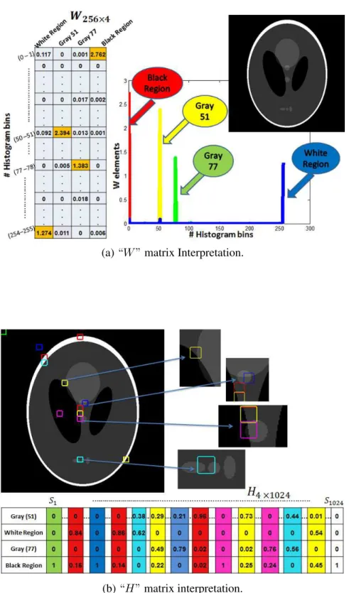
image ; ; ; ; , and intensity value) ...……….………41 Figure 7. “ ” and “�” matrices interpretation for a synthetic gray-scale image with
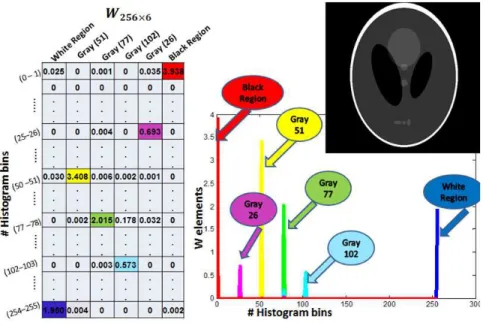
× block size and the entries of “�” normalized for each column...42 Figure 8. “ ” and “�” matrices interpretation for a synthetic gray-scale image with
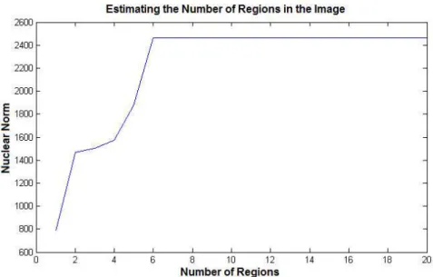
× block size and the entries of “�” normalized for each column ………43 Figure 9. Nuclear norm for the synthetic gray-scale image in Fig. (6) which has six
regions by increasing � from 1 to 20 ………44 Figure 10. Performance evaluation of the proposed PNMF-LSM, the localized-LSM [25] and the improved LGDF-LSM [10] on three synthetic images corrupted with different level of noise and intensity inhomogeneity ……..………..48
List of Figures (continued)
Figure Page
Figure 11. Comparison based on � , and � values between the three methods.49 Figure 12. Robustness of the proposed PNMF-LSM segmentation to contour
initializations ……….53
Figure 13. Segmentation accuracy of the proposed PNMF-LSM approach for different initial contours as measured by the � , and � ……….53 Figure 14. The box plots of the � , and � values for the star object in the
synthetic image obtained from the proposed PNMF-LSM, the localized-LSM and the improved LGDF-localized-LSM for different values of the parameters,
, and ………….………...54
Figure 15. The box plots of convergence times of the three models, the proposed PNMF-LSM, the localized-LSM and the improved LGDF-PNMF-LSM, for different value
of the parameters , and ……….55
Figure 16. PNMF-LSM performance evaluation for different block sizes using the � , and � ...55 Figure 17. Nuclear norm with a block size one for the synthetic gray-scale image in Fig.
(5.3) which has six regions by increasing � from 1 to 20...58 Figure 18. Segmentation of a brain MRI image with Glioblastoma using the proposed
PNMF-LSM approach ………...62
Figure 19. Segmentation of a brain MRI image with Glioblastoma using the proposed
List of Figures (continued)
Figure Page
Figure 20. Segmentation of a brain MRI image with Glioblastoma using the proposed
PNMF-LSM approach ………...63
Figure 21. Segmentation of a normal brain MRI image using the proposed PNMF-LSM
approach ………63
Figure 22. Segmentation of a brain MRI image with Glioblastoma using the proposed PNMF-LSM approach...64 Figure 23. PNMF-LSM segmentation of a brain MRI image with Glioblastoma blurred
by Gaussian noise with standard deviation (2) ...64 Figure 24. PNMF-LSM segmentation of a brain MRI image with Glioblastoma corrupted
by salt and pepper noise...65 Figure 25. Localized-LSM segmentation of a brain MRI image with Glioblastoma …..65 Figure 26. Localized-LSM segmentation of a brain MRI image with Glioblastoma blurred
by Gaussian noise ...66 Figure 27. Localized-LSM segmentation of a brain MRI image with Glioblastoma
corrupted by salt and pepper noise...66 Figure 28. Improved LGDF-LSM segmentation of a brain MRI image with
Glioblastoma...67 Figure 29. Improved LGDF-LSM segmentation of a brain MRI image with Glioblastoma
blurred by Gaussian noise...67 Figure 30. Improved LGDF-LSM segmentation of a brain MRI image with Glioblastoma
List of Tables
Table Page
Table 1. � , and � similarity measures of the three segmentation models, the proposed PNMF-LSM, the localized-LSM and the improved LGDF-LSM, applied on 10 synthetic images………...50 Table 2. � , and � similarity measures of the three segmentation models, the
proposed PNMF-LSM, the localized-LSM and the improved LGDF-LSM, for different values of , and ………...56 Table 3. Convergence time of the three segmentation models, the proposed PNMF-LSM,
the localized-LSM and the improved LGDF-LSM, for different values of the parameters , and (measured in seconds) ……….57 Table 4. � , and � and CPU time (in seconds) of the proposed PNMF- LSM
approach with different block sizes (16 × 16), (8 × 8), (4 × 4), (2 × 2) and (1 × 1) ………..58
Chapter 1 Introduction
In this section, we will motivate and state the problem of medical image segmentation, review the state-of-the-art approaches applied in this field and shed the light on the main contributions of our thesis work.
1.1 Motivation, Problem Statement and Background
Medical image segmentation is one of the most important and complex tasks in medical image analysis and is often the first and the most critical step in many clinical applications, such as surgical planning and image-guided interventions. For instance, in brain MRI anal-ysis, we need to visualize and measure the brain anatomical structures, detect the changes in the brain and delineate the pathological regions. Segmentation of brain MRI images into specific tissue types requires assigning to each element or pixel in the image a tissue label, where the labels are defined in advance. For normal brain, image pixels are typi-cally segmented into three main tissue types: white matter (WM), gray matter (GM) and cerebrospinal fluid (CSF), while in the case of brain tumors, such Glioblastoma, there are additional structures that include the tumor, edema (swelling) and necroses (dead cells).
There are three main challenges with brain MRI segmentation: i) The (normal and ab-normal) brain anatomical structures have complex morphologies and boundaries; ii) The distinct regions of the brain MRI are not homogeneous but present an intensity inhomo-geneity, or bias field. The bias field arises from the spatial inhomogeneity of the magnetic field, the variations in the sensitivity of the reception coil and the interaction between the magnetic field and the human body [37]; and iii) Distinct anatomical structures may have
close average intensity values, e.g., gray-matter and necrosis. These challenges make clas-sical segmentation techniques, such as thresholding [36], edge detection [16], [17], region growing [34], [43], classification [15], [42], [44], and clustering [1], [9], [14] ineffective at accurate delineation of complex boundaries.
Deformable models are ones of the most powerful and advanced methods for image segmentation. The basic idea is to evolve a curve in the image domain around the object or the region of interest until it locks onto the boundaries of the object. The deformable model segmentation problem is formulated and solved using calculus of variations and par-tial differenpar-tial equations (PDEs). Deformable models can be classified into two groups:
snakesoractive contourmodels [6], [12], [20], [21] andlevel setmethods [31], [32], [35]. In the snake or active contour model, the contour is represented in a parameterized form by a set of points that are propagated under the influence of an internal energy and an exter-nal energy. The interexter-nal energy defines the shape of the contour and imposes smoothness and relevant geometrical constraints on the curve. The external energy is computed from the image and attracts the contour towards objects boundaries and other desired features in the image. However, the major drawbacks of the active contour model are its sensitivity to the initial conditions and the difficulties associated with the topological changes for the merging and splitting of the evolving curve. These difficulties actually lie in the parametric representation of the contour. For instance, when the contour merges and splits to fit the objects boundaries in the image, one has to keep track of which points are in which contour and what their order is. The level set approach proposes a geometric (rather than paramet-ric) representation of the contour. Specifically, the contour is represented as the zero level of a higher dimensional function, referred to as the level set function. Instead of tracking
a curve through time, the level set method evolves a curve by updating the level set func-tion at fixed coordinates through time. In particular, since the level set does not have any contour points, the merging and splitting of the curve is done automatically and no new contours need to be defined or removed. The internal and external energies, in the level set approach, are defined in a similar manner as in the active contour method. The power of the level set and active contour methods, referred to as deformable models, stems from their continuous formulation, which can achieve pixel-level accuracy, a highly desirable property in medical image segmentation.
A good body of the work has been done to develop an accurate and robust external energy, also called the data term, that can move the curve and accurately fit the regions boundaries in the image. One of the earliest level set approaches is the Mumford Shah (MS) model [39]. It assumes that the image is piecewise smooth in the areas of objects and backgrounds. However, it is difficult to apply the gradient descent method to solve the MS model because of the non-differentiability with respect to the image boundary. Chan and Vese [7] simplified the MS model using a variational level-set formulation. The Chan-Vese model is based on the assumption that the intensity within each region is homogenous or roughly constant. The image is thus approximated by a constant inside every region. This model, however, is only effective for piecewise constant images and it does not handle intensity inhomogeneity within regions. A major shortcoming of the MS and Chan-Vese models is their assumption of intensity homogeneity within each region of the image.
Recently, local intensity information has been incorporated into the level set methods to effectively handle intensity inhomogeneity. In [26], Li et al. defined a region-scalable fitting (RSF) energy functional as the external energy term of the level set by using a kernel
function with a scale parameter, which allowed the use of local intensity information in image regions at a controllable scale, and two fitting functions that locally approximate the image intensities on the two sides of the contour. The RSF model simultaneously estimates the local intensity mean of each region with the level set function through an iterative pro-cedure. This local definition of regions statistics was the only way to handle the intensity inhomogeneity in the RSF model. In [41], Wanget al. proposed a local Gaussian distri-bution fitting (LGDF) energy with a level set function by also using a kernel function and local means and variances as variables, that were also simultaneously derived with the level set function in an iterative procedure. Both the RSF and LGDF models relied on estimating the local statistics of the image regions through the level set formulation to handle inten-sity inhomogeneity without introducing the bias field as a separate variable to correct for the intensity inhomogeneity in the original image. More recent applications of the level set approach, which also took into account the intensity inhomogeneity, defined a local clustering criterion for the image intensities in a neighborhood of each pixel. This local clustering was then integrated to give a global criterion of image segmentation, and served as the external energy term of the level set formulation. These methods used localized clus-tering (Localized-LSM) [25], and statistical characteristics of local intensities (Improved LGDF-LSM) [10]. Obviously, the performance of the level set approach depends on the lo-cal clustering criterion used. These two methods added the bias field as a separate variable estimated through the variational principle of the level set formulation in order to correct for the intensity inhomogeneity in the original image. Multiplying the local average in-tensity of each region inside the neighborhood by the bias field variable gives us different intensity values in the same region and thus handles the intensity inhomogeneity in every
region. Moreover, each local clustering criterion has its own parameters that have to be simultaneously estimated along with the level set function and the bias field. For instance, in the localized level set clustering criterion (Localized-LSM) in [25], the local intensi-ties in every region have to be estimated along the bias field and the level set functions. Similarly, the statistical approach (Improved LGDF-LSM) in [10] involved simultaneous and iterative estimation of the mean and variance and other parameters of the local density approximation.
All previously mentioned approaches involved simultaneous and iterative estimation of a number of model parameters in addition to the bias field and the level set function, which is the main parameter to be estimated. Given the high-dimensionality and non-convexity of the variational optimization problem, all additional model parameters are estimated in an iterative procedure that does not guarantee convergence or optimality of the results. Hence, one of the drawbacks of these state-of the-art approaches is the number of model param-eters that are introduced, and have to be simultaneously estimated, which decreases the estimation accuracy of the main segmentation parameters, namely the level set functions. Moreover, all recent level set approaches are built based only on the first and second order statistical features: the mean and standard deviation intensities of the pixel values. More-over, these features do not incorporate any information on the spatial distribution of the pixel values which may greatly improve the segmentation.
1.2 Research Contributions
This thesis contributes to the field of (medical) image segmentation by introducing a new deformable model that is able to delineate complex boundaries of image regions by relying
on the image density information (histogram) rather than the absolute pixel intensity val-ues and correcting for the intensity inhomogeneity without introducing additional model parameters to be estimated simultaneously with the level set functions. The proposed seg-mentation framework has four advantages compared to the state-of-the-art: i) less sensitive to the model parameters, ii) more robust to noise in the image, iii) less sensitive to the initial contour, and iv) has a higher convergence rate. Specific contributions of this work include:
• Building the data matrix using the histograms of the image blocks rather than relying on the absolute pixel intensity values. This characterization makes the subsequent algorithm more robust to noise in the image.
• Elucidating how the non-negative matrix factorization (NMF) of the data matrix can cluster the image into distinct regions, and how relevant image structures can be extracted from the NMF factors.
• Deriving a measure based on the nuclear norm of the NMF factors to estimate the number of distinct regions in the image.
• Introducing two new external energy or data terms derived from the two factors of the NMF. In particular, introducing a new spatial term, which increases the resolution of the proposed algorithm by increasing its ability to discriminate between distinct regions with close average intensity values.
• Proposing a new NMF-based level set method with the bias field correction to take into account intensity inhomogeneity. The proposed model does not require the es-timation of spurious model parameters in addition to the bias field and the level set
functions.
• Incorporating the statistics of noise in the data by using probabilistic non-negative matrix factorization (PNMF) given in [4], which assumes that the data matrix is corrupted by additive white Gaussian noise.
1.3 Organization
This thesis is organized as follows.
In Chapter 2, we provide a literature review of the state-of-the-art level set models, describing their mathematical formulation and model parameters. It is crucial to understand the mathematical and theoretical assumptions of the previous work in order to grasp the novelty of this thesis.
In Chapter 3, we review the mathematical and theoretical formulation of the non-negative matrix factorization (NMF) and its variants, including probabilistic NMF (PNMF). PNMF assumes that the data matrix is not deterministic but corrupted by additive white Gaussian noise. We subsequently explain how NMF can be used to discover the image regions and cluster them.
In Chapter 4, we review the mathematical and theoretical formulation of the level set method (LSM), including the level set membership functions that partition the image do-main into disjoint, non-overlapping regions.
In Chapter 5, we introduce the proposed PNMF-LSM approach. We describe how the positive factors of the PNMF discover and cluster the image domain into distinct regions. We introduce two external energy terms that will drive the contour to the regions
bound-aries. We take into account the bias field and carry out the segmentation by minimize the total energy functional with respect to the level set functions.
In Chapter 6, we provide and discuss the simulation results by evaluating the perfor-mance of the proposed PNMF-LSM method as compared to two other state-of-the-art level set methods, the localized level set model (localized-LSM) [25] and the improved LGDF level set model (improved LGDF-LSM) [10]. We study the robustness of the models to the model parameters, initial conditions and noise introduced in the image. We also discuss the convergence time of the models.
In Chapter 7, we apply the proposed PNMF-LSM method to real brain MRI images, with and without tumor, to delineate the complex structures of the brain: gray matter, white matter, cerebrospinal fluid (CSF), edema (swelling), tumor and necroses (dead brain cells). We also show the robustness of our method to blurring by Gaussian kernels and to salt and pepper noise.
Chapter 2 Literature Review
In this chapter, we will review the state-of-the-art in level set methods that build differ-ent data terms (or external energies) in the level set framework for image segmdiffer-entation.
2.1 Mumford-Shah Model [39]
Let Ω be the image domain, and I : Ω → R be a gray-value image. The goal of the segmentation is to find a contour C, which separates the image domain Ω into disjoint
regionsΩ1,· · ·,Ωk, and a piecewise smooth functionuthat approximates the imageIand
is smooth inside each regionΩi. This is formulated as the minimization of the following
Mumford-Shah functional: FM S(u, C) = Z Ω (I−u)2dx+µ Z Ω\C |∇u|2dx+ν|C|, (2.1)
where|C|is the length of the contourC. In the right hand side, the first term is the external energy term, which drivesuto be close to the imageI, and the second term is the internal energy, which imposes smoothness on u within the regions separated by the contour C. The third term regularizes the contour. The MS model is very general and does not assume a specific form for the approximating function u. It also assumes that the objects to be segmented are homogeneous.
2.2 Chan and Vese Model [7]
Chan and Vese simplified the Mumford-Shah model by assuming that the approximating functionuis a piecewise constant:
FCV(φ, c1, c2) = Z Ω |I(x)−c1|2H(φ)dx + Z Ω |I(x)−c2|2(1−H(φ))dx+ν Z Ω |∇H(φ)|dx, (2.2)
whereH is the Heaviside function, andφis a level set function, whose zero level contour
C partitions the image domain Ω into two disjoint regions Ω1 = {x : φ(x) > 0} and
Ω2 ={x:φ(x)<0}. Equation (2.2) is a piecewise constant model, as it assumes that the
imageI can be approximated by constants ci in region Ωi. In the case of more than two
regions, two or more level set functions can be used to represent the regionsΩ1,· · ·Ωk.
2.3 Localized-LSM Model [25]
In [25], Liet al. proposed a variational level set method that deals with intensity inhomo-geneity by considering the following model for the observed imageI:
I =b∗J +n, (2.3)
whereb is the bias field,J is the true image andnis the additive noise. This approach has two assumptions: a) the bias field is assumed to be slowly varying, and b) the true image
J is approximated by a constant inside each region: J(x) ≈ ci forx ∈ Ωi. Consider the
neighborhoodOy. The energy function is then formulated as the following [25]: F(φ,b,c) = Z N X i=1 Z K(y−x)(I(x)−b(y)ci)2Mi(φ(x))dx ! dy, (2.4)
where K(y−x) is a non-negative weighting function that defines the neighborhood Oy,
Mi(φ(x))is the membership function that represents each region using the Heaviside
func-tion, (for two regionsM1(φ) = H(φ), and M2(φ) = 1 −H(φ)). In the localized-LSM
model, the intensity means c1,· · ·, ck of each region are estimated iteratively along with
the level set functionφ and the bias fieldb using the variational principle of the level set framework.
2.4 Improved LGDF-LSM Model [10]
In the Improved LGDF-LSM model [10], Chen et al. characterize the local distribution of the intensities in the neighborhood Ox using a local Gaussian distribution. The
seg-mentation is then achieved by maximizing the a posteriori probability. They used the log transform of the same image model in Li’s methodIe=log(I) = log(J) +log(b)so that
the bias becomes an additive factor rather than a multiplicative factor.
Let p(x ∈ Ωi ∩ Ox|Ie(x)) be the a posteriori probability of the subregions Ωi ∩ Ox
given the log transform of the observed image. Using Bayes’ rulep(x ∈Ωi∩Ox|Ie(x))∝
p(Ie(x)|x∈Ωi∩Ox)p(x∈Ωi∩Ox). Assuming that the prior probabilities of all partitions
are equal, and the pixels within each region are independent, the MAP estimate can be achieved by finding the maximum ofQNi=1Qx∈Ωi∩Oxpi,y(Ie(x)). It can be shown that the
in the level set framework: F(φ,b,c, σ2) = Z N X i=1 Z −K(y−x) logpi,y(Je(x)−eb(y))Mi(φ(x))dxdy, (2.5)
where pi,y(Je(x)−eb(y)) is modeled by a Gaussian distribution. In the improved LGDF
model the intensity means {ci}ki=1 and variances {σi2}ki=1 of each region are
simultane-ously and iteratively estimated with the level set functionφ, and the bias fieldbusing the variational principle of the level set framework.
Chapter 3
Non-Negative Matrix Factorization
In this chapter, we review the theoretical and mathematical formulation of the non-negative matrix factorization and some of its variants. Then, we shed the light on the NMF as a clustering technique.
3.1 NMF and Its Variants
3.1.1 Standard-NMF. Non-negative matrix factorization (NMF) is a matrix decom-position approach which decomposes a non-negative matrix into two low-rank non-negative matrices. It was introduced as a dimensionality reduction method for pattern analysis [24]. When a set of observations is given in a matrix with nonnegative elements, NMF seeks to find a lower rank approximation of the data matrix, where the factors that give the lower rank approximation are also non-negative. The non-negativity constraint is re-quired in some applications in order to obtain physically meaningful results and interpreta-tions. Mathematically, the problem is formulated as follows: Given a non-negative matrix
V ∈ Rn×m, NMF provides two non-negative matricesW ∈ Rn×k and H ∈ Rk×m such thatV ≈W H. The optimal factors minimize the squared error and are the solutions to the following constrained optimization problem,
min
W,H f(W, H) = kV −W Hk
2
F, subject toW, H ≥0, (3.1)
wherek.kF denotes the Frobenius norm andf is the squared Euclidean distance function
between V and W H. Observe that the cost function f is convex with respect to one of the variablesW orH, but not both. Alternating minimization of such a cost leads to the
Alternating Least squares (ALS) algorithm [22], which can be described as follows:
1. InitializeW randomly or by using any a priori knowledge.
2. EstimateH asH = (WTW)−WTV with fixedW.
3. Set all negative elements ofHto zero or some small positive value.
4. EstimateW asW =V HT(HHT)−
with fixedH.
5. Set all negative elements ofW to zero or some small positive value.
In this algorithm,A−denotes the MoorePenrose inverse ofA. The ALS algorithm has been used extensively in the literature [2], [18]. However, it is not guaranteed to converge to a global minimum nor even a stationary point. Moreover, it is often not sufficiently accurate, and it can be slow when the factor matrices are ill-conditioned or when the columns of these matrices are co-linear. Furthermore, the complexity of the ALS algorithm can be high for large-scale problems as it involves inverting a large matrix [4]
Lee and Seung [23] proposed a multiplicative update rule, which is proven to converge to a stationary point, and does not suffer from the ALS drawbacks. The multiplicative update rule of the Lee and Seung’s algorithm is shown in Eq. (3.2) as a special case of a class of update rules, which converge towards a stationary point of the NMF problem.
Hij ←Hij (W TV) ij (WTW H) ij Wij ←Wij (V H T) ij (W HHT) ij. (3.2)
Iteration of these update rules converges to a local maximum of the objective function:
F = n X i=1 m X j=1 [Vijlog(W H)ij −(W H)ij]. (3.3)
The update rules preserve the non-negativity ofW andHand also constrain the columns of
W to sum to unity. This sum constraint is a convenient way of eliminating the degeneracy associated with the invariance ofW Hunder the transformation W → WΛ, H →Λ−1H,
whereΛis a diagonal matrix.
3.1.2 Sparse-NMF. Sparsity is a popular regularization principle in statistical mod-eling [38], and has been used to reduce the non-uniqueness of solutions and also to enhance the interpretability of the NMF results. The sparse-NMF proposed in [29] imposes sparsity on the factor matrixHby constraining thel1-norm of its columns and imposes a unity-norm
on the columns ofW to ensure the uniqueness:
min W,Hf(W, H) =kV −W Hk 2 F +λ n X i=1 khik1 (3.4) subject toW, H ≥0,kwik22 = 1, i= 1, ..., k.
The optimization problem in Eq. (3.4) is solved in [29] using non-negative quadratic pro-gramming (NNQP).
For a more comprehensive overview of the different variants of NMF, including Versa-tile sparse matrix factorization and Kernel-NMF, the reader is referred to [29].
3.1.3 Probabilistic Non-Negative Matrix Factorization PNMF [4]. In [4], It is assumed that the data, represented by the non-negative matrixV, is corrupted by additive white Gaussian noise, and follows the following conditional distribution,
p(V|W, H, σ2) = N Y i=1 M Y j=1 N(Vij|uTi hj, σ2), (3.5)
whereN(.|µ, σ2)is the probability density function of the Gaussian distribution with mean
µand standard deviationσ,ui, andhj denote, respectively, theithrow of the matrixW and
thejth column of the matrixH. Zero mean Gaussian priors are with standard deviations
σW andσH, respectively, imposed onui andhj to control the model parameters. W, and
Hare estimated using MAP criterion by minimizing the following function:
f(W, H) = kV −W Hk2F +αkWk2F +βkHk2F, subject toW, H ≥0, (3.6)
where the parametersαandβdepend onσ, σW andσH. It was shown that the update rules
for the optimization problem in (3.6) are given by [4],
Hij ←Hij (WTV) ij (WTW H+βH) ij Wij ←Wij (V HT) ij (W HHT+αW) ij. (3.7)
Observe that, since the data matrixV is negative, the update rules in (3.7) lead to non-negative factors W andH as long as the initial values of the algorithm are chosen to be non-negative.
3.2 NMF as a Clustering Technique
In [5], NMF was used to extract relevant biological correlations in gene expression data. The data was represented by an expression matrixAof sizeN ×M, whose rows contain the expression levels of N genes inM samples. The NMF reduces the dimensionality of the gene expression data into a small number (k < N) of “metagenes”, defined as positive linear combinations of theN genes. Then, the gene expression pattern of the samples are approximated as positive linear combinations of these metagenes. Mathematically, this corresponds to factoring the matrixA into two matrices with positive entries,A ≈ W H.
MatrixW has sizeN ×k, with each of thekcolumns defining a metagene; Thewij entry
is the coefficient of geneiin metagenej. MatrixH has size k×M, with each of theM
columns representing the metagene expression pattern of the corresponding sample; The
hij entry represents the expression level of metagene iin samplej. Given a factorization
A ≈ W H, the matrix H is used to group M samples into k clusters. Each sample is placed into a cluster corresponding to the most highly expressed metagene in the sample; that is, sample j is placed in cluster i if the hij is the largest entry in column j; (see
Fig. (1)). In [24], Lee et al. used the NMF to decompose images of human faces into
Figure 1. Rank-2 reduction of a DNA microarray ofN genes andM samples is obtained by NMF,A ≈ W H. Metagene expression levels (rows of H) are color coded by using a heat color map, from dark blue (minimum) to dark red (maximum). The same data is shown as continuous profiles below. The relative amplitudes of the two metagenes determine two classes of samples, class 1 and class 2. Here, the samples were ordered to better expose the class distinction [5].
parts reminiscent of features such as eyes and noses, while the application of traditional factorization methods, such as principal component analysis (PCA) and vector quantization (VQ), to the image data yielded components with no obvious interpretation. The database of images is viewed as an n×m matrixV, where each column contains n non-negative pixel values of one of themfacial images. The NMF leads to the decompositionV ≈W H, where the dimensions of the factorsW andH aren×r and r×m, respectively. The r
columns ofW are termed “basis images”. Each column ofH is called anencodingand is in one-to-one correspondence with a face in V. An encoding consists of the coefficients by which a face is represented as a linear combination of basis images. The NMF basis and encodings contain a large fraction of vanishing coefficients. Both the basis images and the image encodings are sparse. The basis images are sparse because they are “non-global” and contain several versions of mouths, noses and other facial parts, where the various versions are in different locations or forms. The variability of a whole face is generated by combining these different parts. Although all parts are used by at least one face, any given face does not use all the available parts. This results in a sparsely distributed image encoding, in contrast to the unary encoding of VQ and the fully distributed PCA encoding [24] as shown in Fig. (2).
Figure 2. Non-negative matrix factorization (NMF) learns a parts-based representation of faces, whereas vector quantization (VQ) and principal component analysis (PCA) learn holistic representations. The three learning methods find approximate factorizations of the formV ≈W H, but with three different types of constraints onW andH. As shown in the
7×7montages, each method has learned a set ofr = 49basis images. Positive values are illustrated with black pixels and negative values with red pixels. A particular instance of a face, shown at top right, is approximately represented by a linear superposition of basis images. The coefficients of the linear superposition are shown next to each montage, in a
7×7grid, and the resulting superpositions are shown on the other side of the equality sign. Unlike VQ and PCA, NMF learns to represent faces with a set of basis images resembling parts of faces, such as eyes, mouth and nose [24].
Chapter 4 Deformable Models
In this chapter, we explain the detailed theoretical and mathematical formulation of the two classes of deformable models: the parametric deformable model, also known assnake
oractive contour, and the geometric deformable model, also known as thelevel set method. Deformable models refer to a powerful class of physics-based modeling techniques widely employed in the image synthesis, image analysis, image segmentation, shape de-sign and related fields. By numerically simulating the governing equations of motion, typi-cally expressed as Partial Differential Equations (PDEs) in a continuous setting, deformable models mimic various generic behaviors of natural non-rigid materials in response to ap-plied forces, such as continuity, smoothness and elasticity. Deformable models offer a potent approach that combines geometry, physics and approximation theory. Such models can be used to infer image disparity fields, image flow fields, and to infer the shapes and motions of objects from static or video images. In this context, deformable models are sub-ject to external forces that impose constrains derived from image data. The forces actively shape and move the model to achieve maximal consistency with the objects of interest and maintain consistency over time. These models are widely used in medical image analy-sis; they have proven to be very useful in segmenting, matching and tracking anatomic structures by exploring constraints derived from the image data in conjunction with a priori knowledge about the location, size and shape of these structures [32]. There are two types of deformable models: parametric and geometric models. Parametric deformable models represent curves and surfaces explicitly in its parametric form, i.e., using a set of contour points. Its popularity in medical image analysis is credited to the work of snake or (active
contour) by [20]. The geometric deformable model (level set method) is based on the the-ory of curve evolution and geometric flow, which represents curves and surfaces implicitly as a level set of an evolving higher dimensional function [19].
4.1 The Parametric Deformable Model (Snake or Active Contour)
Active contour models (ACMs) are based on the idea of evolving a curve in the image domain under the influence of an internal energy and an external energy [20]. The optimal contour minimizes the total energy functional, given by the weighted sum of the internal energy and external energy terms. This curve is represented in a parameterized form by a set of contour points. The internal energy defines the shape of the contour and imposes smoothness and relevant geometrical constraints on the curve, e.g., Eq. (4.1). In Equation (4.1), υ(s) denotes the parameterized curve, where the points (x(s), y(s)) move through
the spatial domain of the image to minimize the energy functional, and w1, w2 are the
weighting parameters that control the contour’s elasticity and rigidity. The external energy in Eq. (4.2) is computed from the image and attracts the contour towards objects boundaries and other desired salient features in the image. The total active contour energy functional is given in Eq. (4.3). This model is used for image segmentation and some other applications in image processing, such as edge detection, shape modeling and motion tracking [20].
EInternal = w1(s) 2 |υ 0 (s)|2+w2(s) 2 |υ 00 (s)|2, (4.1) EExternal =−|∇I(υ(s))|2, (4.2)
EACM =EInternal+EExternal = w1(s) 2 |υ
0(s)|2+ w2(s)
2 |υ
00(s)|2− |∇I(υ(s))|2.
In order to minimize the total energy EACM, we formulate this functional as a
Euler-Lagrange functionalL(s, υ(s), υ0(s), υ00(s))and solve the Euler-Lagrange equation of the
general form: F(f) = Z x1 x0 L(x, f(x), f0(x), f00(x), ..., fn(x))dx, f0 = df dx, f 00 = d 2f dx2, f n= dnf dxn. (4.4) The stationary values of the functionalF(f) in Eq. (4.4) can be obtained by solving the
Euler-Lagrange equation [8]: ∂L ∂f − d dx( ∂L ∂f0) + d2 dx2( ∂L ∂f00)−....+ (−1) n dn dxn( ∂L ∂fn) = 0. (4.5)
By adding the time variable, it can be shown that minimizingEACM corresponds to solving the following Euler-Lagrange equation.
υt(s, t) =−(w1υ0)0+ (w2υ00)00+∇EExternal(υ) = 0, (4.6)
where υt = ∂υ∂t. The finite difference equation in (4.6) can be solved numerically using
gradient descent.
4.2 Drawbacks of the Active Contour Model
There are two main difficulties in the active contour model: First, the contour must be ini-tialized fairly close to the final target in order to converge. However, to make a “good” initialization, we need to have a “good” estimate of the solution before starting the itera-tive process of adapting the contour. This leads to a solution that is sensiitera-tive to the initial condition. Secondly, there are difficulties associated with the topological changes for the merging and splitting of the evolving curve. These difficulties lie in the parametric repre-sentation of the contour. For instance, when the contour merges and splits to fit the objects’
boundaries in the image, one has to keep track of which points are in which contour and what their order is. Figure 3 shows an example, where the active contour model fails in handling the topological changes associated with the movement of the fingers [13].
Figure 3. The active contour model fails to handle the topological changes of the moving fingers [13].
4.3 The Level Set Method
The basic idea of the level set method [33], [31] is to embed the moving contour as the zero iso-contour of a higher-dimension implicit functionφ :Rn×R+ −→R. In the 2D spatial
dimension, the closed curve, denoted byC, can be implicitly represented as the zero level
set function follows the Hamilton- Jacobi equation: ∂φ ∂t +F|∇φ|= 0 φ(x, y,0) =φ0(x, y), (4.7)
where the functionF, called thespeed function, is defined depending on the mean-curvature [33] or image edges information [6]. In the early implementations of the level set method [30], [31], the level set function φ can develop discontinuous jumps, known as shocks, during the evolution, which makes further computation highly inaccurate. To avoid these problems, a common numerical scheme is to initialize the functionφas a signed distance function before the evolution, and then “reshape” (or “re-initialize”) the functionφto be a signed distance function periodically during the evolution. It is crucial to keep the evolving level set function as an approximate signed distance function during the evolution, espe-cially in a neighborhood around the zero level set. It is well known that a signed distance function must satisfy a desirable property of |∇φ| = 1. Conversely, any function φ sat-isfying |∇φ| = 1 is the signed distance function plus a constant. In order to avoid the drawbacks of the re-initialization procedure, Liet alproposed in [27] a variational level set formulation that does not require o the re-initialization procedure by using the following integral:
R(φ) =
Z
Ω
0.5(|∇φ| −1)2dx, (4.8)
as a metric to characterize how close a functionφis to a signed distance function. Then the level set variational formulation is given by:
whereµ > 0is a parameter controlling the effect of penalizing the deviation of φ from a
signed distance function, andEm(φ)is a certain energy that would drive the motion of the
zero level curve ofφ.
Using calculus of variation, the evolution of the level set function is given by:
∂φ ∂t =−
∂E
∂φ. (4.10)
For the purpose of image segmentation,Emis defined as a functional that depends only on
the image data, and is, therefore, called theexternal energy. Accordingly, the energyR(φ)
is called theinternal energyof the functionφ, since it is a function ofφonly [27]. We can also add other smoothing constraints to the energy functionalE.
Chapter 5
NMF-Based Level Set Segmentation
In this chapter, we will show how the NMF can be used to discover the image regions and estimate their number. We will present the theoretical and visual interpretations of the
W, andH factors of the NMF and explain how they can be used to build a robust energy functional of the image. The proposed NMF-based level set model is subsequently derived.
5.1 Region Discovery using NMF
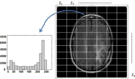
We first construct a data matrix based on the histogram of the image, rather than the inten-sity values directly. This data matrix takes into account the local information in the image by partitioning the image intomblocks and computing the histogram of each block. The histograms of the blocks are then stacked to form the columns of the data matrixV. The data matrixV ={υij}is ann×mmatrix, wherenis the number of intensity bins or ranges
in the histograms standardized for all image blocks. Specifically, the (i, j) entry,υij, is the
number of pixels in the block j with intensity range in the bini. The rows of V describe the ranges of intensity in the bin i in every j block. Our goal is to find k < m “basic histograms” such that the histogram of every image block can be expressed as a positive linear combination of the basic histograms. This can be achieved using non-negative ma-trix factorization (NMF). NMF provides a natural way to cluster the histogram data mama-trix, because it involves nonnegative entries. Other matrix decomposition techniques, such as principal component analysis (PCA) or singular value decomposition (SVD) do not guar-antee the non-negativity constraints, and hence loose the physical and intuitive interpreta-tion of the factorizainterpreta-tion. However, this non-negativity requirement makes the factorizainterpreta-tion
problem more challenging, as we saw in Chapter 3. We use the Probabilistic NMF (PNMF) algorithm in [4], which takes into account the noise in the data matrix and performs a max-imum a posteriori NMF factorization. This algorithm was presented in Chapter 3 Section 3.1.3.
Mathematically, the task of finding the basic histograms of the image corresponds to factoring the histogram data matrix V into two matrices with positive entries V ≈ W H, whereW isn×kandHisk×m. Thekcolumns ofW define the basic histograms, which we will show, correspond to the histograms of the distinct image regions. Thekrows of the matrixHcluster the data matrix into metabins, and represents the distribution of the image regions within themblocks. An illustration of the NMF factorization of the data matrix is provided in Fig. (4).
The PNMF factorization V ≈ W H induces then a clustering of the histogram data matrix intok basic histograms or k metabin regions Ωi, i = 1,· · · , k. In the sequel, we
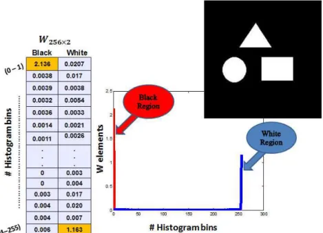
will investigate how the non-negative matrices W and H provides statistical and spatial information about the clustered regions in the image. We first consider the synthetic binary image in Fig. (5). The PNMF of the data matrix of this image with k = 2 results in
theW and H matrices shown in Fig. (5a), (5b), respectively. Plotting the entries of each column of W, we obtain two sharp peaks: one peak at the (0 − 1) range of intensity value, corresponding to the black region, and a second peak at the (254 − 255) range, corresponding to the white region. Hence, the matrixW seems to provide the distribution of the pixel intensity values in each region, and from this distribution, we can obtain the statistical information (mean and variance of every region in the image). The normalized entries of the columns ofH provide the percentage of pixels in every block that are within
(a) Dividing the image into blocks and computing the histogram of each block.
(b) Data matrix and histogram factorization.
the clustered regions of the image. For instance, when the image block is included entirely in one region, we obtain the value of1in the entry that corresponds to that region and zero
in the other. While, if two regions are included in the block, we obtain the exact percentages of the local areas of these regions in that block (see Fig. (5b)).
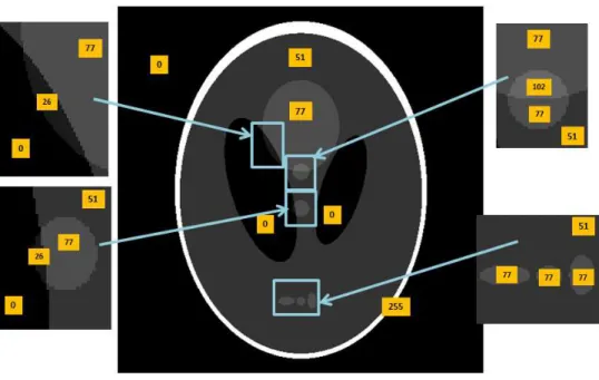
The same interpretation has been reached on the synthetic gray-scale image given in Fig. (6). For this synthetic image, we started by meshing the image into N ×N blocks first (N = 16in this case). From the plot of the columns of the matrixW in Fig. (7a), we
observe that the PNMF captured the four large regions in the image, while the two small regions in the image with intensity values(102)and(26)were not detected. BothW and
H matrices were unable to capture these two small regions with a block size of (16×16). Even when we increase the number of regions k, we get additional zero columns in W, and additional zero rows in H, thus unable to capture these two small regions. However, by decreasing the size of the blocks to (8×8), so that the block size fits into these small regions, we found that the W and H matrices of the PNMF factorization specified six regions including the two small regions, as shown in Fig. (8). Hence, by decreasing the block size to partition the image and build the data matrixV, the PNMF resolution ability to distinguish small regions increases. The resolution of the PNMF is thus directly related to the block size used when partitioning the image. In other words, the smallest distinct region that can be detected by the PNMF has a size approximately equal to the block size.
In summary, applying the probabilistic non-negative matrix factorization PNMF on the histogram data matrix, that we build in section 5.1, provides two positive matrices that pro-vide the statistical and spatial characteristics of the image regions. The matrixW provides the histogram distribution of each region in the image, which means that we can obtain the
(a)“W”matrix Interpretation.
(b)“H”matrix interpretation.
Figure 5. “W”and“H”matrices interpretation for a synthetic binary image with16×16
statistical mean and variance of each region; While the matrixHprovides the local spatial characteristics of each region: the percentage area of each region that is included in every block size. Based on these statistical and spatial characteristics of the image regions, we propose to build a robust external energy or a data term that will be used in the level set approach.
5.1.1 Estimating the number of distinct regions in the image. We show how to use the factor matricesW andH to estimate the number of distinct clusters or regionsk. To illustrate the idea, we start by changing the value ofkfor the synthetic gray-scale image in Fig. (6) and observing the corresponding changes in the matricesW andH. We notice that when we increasek to be more than the true number of regions in the image (which is in this casek = 6), we obtain additional zero rows inH and additional zero columns in
W. We, therefore, propose to use the sum of thenuclear norms (also known as the trace norms) ofW andH. The nuclear norm of the matrixAis defined as
kAk∗ =trace( √ AHA) = min{m,n} X i=1 σi, (5.1)
where theσis are the singular values of the matrixA. We start by choosing an initial guess
for the number of regionsk0 and we apply the PNMF on the histogram data matrixV with
k = k0. We obtainVn×m ≈ Wn×k0Hk0×m. We compute the sum of the nuclear norms
of Wn×k0 and Hk0×m. Then, we increase k and repeat the same steps. The sum nuclear
norm is a nondecreasing function ofk. This function platforms whenk ≥k∗. The optimal number of regions is then given byk∗.
Fig. (9) shows how the sum of the nuclear norms increases with k for the synthetic gray-scale image in Fig. (6), until it stabilizes at k = 6, which corresponds to the exact
number of regions in the image.
The idea behind using the nuclear norm is that appending the matrixW, having singular values{σi}ki=1, by a column of zeros,zw, and forming the matrixW˜a = [W,zw]will add
a zero singular value. In other words, the singular values ofW˜aare given by{{σi}ki=1,0}.
Thus, the nuclear norm does not change when we add a column of zeros. Similarly, ap-pending the matrixH by a row of zeros, zt
h, and forming the matrixH˜a =
H
zt h
, will not change the sum of the singular values. In practice, we do not have exact zeros in the addi-tional columns and rows of the appended matricesW˜a andH˜a, respectively, but we have
small values that are close to zero. We will show that if the column vectorzw and the row
vectorzth have small entries, then the additional singular values in the appended matrices, ˜
WaandH˜a, are also small. In particular, the nuclear norm will change only slightly when
we append a column or a row of small values. The following lemma formalizes and proves this result.
Lemma 1. Let W ∈ Rn×k andH ∈
Rk×m, where k < min{n, m}. Let {σiW}ki=1 and {σiH}k
i=1 be the singular values ofW andH, respectively. Consider the augmented
ma-tricesWa= [W|0]andHa =
H
0t
, where0denotes the vector with zero entries. Then kWak∗ =kWk∗ and kHak∗ =kHk∗. (5.2) Similarly, consider the augmented matricesW˜ a= [W|zw]andH˜a=
H
zth
, wherezwand
zh are vectors. Then, we have
kWk∗ ≤ kW˜ ak∗ ≤ kWk∗+kzwk, (5.3)
kHk∗ ≤ kH˜ak∗ ≤ kHk∗+kzhk. (5.4)
In particular, ifkzwk ≤ε, andkzhk ≤ε0, then
0≤ kW˜ ak∗− kWk∗ ≤ε, (5.5)
0≤ kH˜ak∗− kHk∗ ≤ε0. (5.6)
5.1.2 Proof of Lemma 1. We will first prove that appending the matrix W by a
column of zeros and the matrixHby a row of zeros will not change the sum of the singular
values of the appended matricesWaandHa.
We have,
{σWa
i }
k
i=1 ={λi(WatWa)}ki=1, (5.7)
where{λi(WtaWa)}ki=1 are the eigenvalues of the matrixW
t aWa, WtaWa= Wt 0t ∗[W|0] = WtW 0 0t 0 ; (5.8)
polyno-mial:
det(WtaWa−λI) =−λdet(WtW −λI) = 0. (5.9)
Then
λ(WtaWa) ={λ(WtW),0} ⇒σ(Wa) = {σ(W),0}. (5.10)
Similarly, we can show that ifHa =
H 0 , thenλ(HaHta) ={λ(HH t),0} ⇒σ(H a) = {σ(H),0}.
We now prove the second part of the Lemma, namely, Eqs. (5.3) and (5.4). First, we can write the appended matrixW˜ aas follows:
˜
Wa = [W|zw] = [W|0n×1] + [0n×k|zw], (5.11)
where the first zero in[W|0n×1]is an×1vector, while the second zero in [0n×k|zw]is a
matrix with the same dimension asW. Using the triangular inequality, we have
kW|zwk∗ ≤ kW|0k∗+k0|zwk∗. (5.12)
We can easily see thatk0n×k|zwk∗ =kzwkand from the first part of the proof,kW|0n×1k∗ = kWk∗. Thus,
kW|zwk∗ ≤ kWk∗+kzwk. (5.13)
In particular, small values ofzw result in a small perturbation of the nuclear norm ofW˜ a.
In order to prove the left hand side of the Eqs. (5.3), (5.4) we use the determinant
formula for block matricesdet
A B C D
= det(A) det(D−CA−1B). We have
˜ WtaW˜ a−λI = Wt zt w ∗[W|zw]−λI = WtW −λI Wtzw ztwW kzwk2−λ . (5.14)
Using the determinant formula we can write the determinant ofW˜ taW˜ a−λI as follows det WtW −λIdet kzwk2−λ−ztwW(W tW −λI)−1Wtz w = 0, (5.15) ⇒ det WtW −λI= 0, det kzwk2−λ−ztwW(W tW −λI)−1Wtz w = 0⇒λ∗ ≥0. . (5.16)
Hence, the eigenvalues ofW˜ taW˜ aare{λ(WtW), λ∗}, whereλ(WtW)are the
eigenval-ues ofWtW andλ∗ ≥0becauseWtW is a positive semi-definite matrix.. Then
kW˜ ak∗ = X i σi(W˜ a) = X i σi(W) + √ λ∗ ⇒ kW˜ ak∗ ≥ kWk∗. (5.17)
Similarly, for the matrix H, we can use the triangular inequality and the determinant
formula of the block matrices to prove the following:
kHk∗ ≤ kH˜ak∗ ≤ kHk∗+kzhk. (5.18)
5.2 Proposed Variational Framework
We consider the image modelI(x) = J(x)∗b(x) +n(x), whereI(x) is the observed intensity at pixelx,J(x)is the “true” (noiseless/unbiased) intensity at pixelx,b(x)is the
bias field associated withx and n(x)is the observation noise. We take into account the
two matricesW andHin the PNMF factorizationV ≈W H to build the proposed energy functional. This functional codes the external energy and contains two terms: a statistical term and a spatial term. The statistical term uses the matrixW and characterizes the mean and standard deviation of the histogram of each region. The spatial term relies on the matrixH and characterizes the local spatial area of each region inside the blocks. In order
to compute the statistical energy term, we formulate the segmentation problem as one of computing the maximum a posteriori (MAP) partition of the image domainΩinto disjoint
regions by maximizing the posterior probability p({Ω1,Ω2,· · · ,Ωk}|I) for the image I.
According to the Bayes rule
p({Ω1,Ω2,· · · ,Ωk}|I)∝p(I|{Ω1,Ω2,· · · ,Ωk})p({Ω1,Ω2,· · ·,Ωk}). (5.19)
Assuming that the prior probabilities of all partitions p({Ω}) are equal, and the pixels within each region are independent, the MAP estimate reduces to finding the maximum of Qk
i=1 Q
x∈Ωipi(I(x)), where pi(I(x)) = p(I(x)|Ωi), i = 1,2, ..., k. By taking the logarithm, the maximization can be converted to the minimization of the following energy function: EStatistical = k X i=1 Z Ωi −logpi(I(x))dx, (5.20)
wherepi(I(x))is modeled as a Gaussian distribution.
pi(I(x)) = 1 √ 2πσi exp(−(I(x)−µib(x)) 2 2(σi)2 ), (5.21)
whereµi, and σi are computed form the matrixW. To compute the spatial energy term,
we consider the matrix H, which induces a local spatial clustering of the regionsΩi, i =
1,· · · , k in each block. Ideally, if the block j is included entirely in the region i, then
hij = 1, and hlj = 0 for l 6= i. Hence, by dividing the entries of H by the sum of
each column, we can interpret hij as the proportion of the area of region i in the block
j. Therefore, we can represent the local spatial area of each region i inside the block j
as a weighted linear combination of the block area where the weights are given by the normalized entries of the jth column of the matrix H. We propose the following spatial
data term: ESpatial = k X i=1 m X j=1 Z Ωi ISj(x)dx− hija Pk i=1hij !2 , (5.22)
whereais the area of each block (all blocks are assumed to have equal areas), andISj(x) is the characteristic function that introduces all pixels in the block Sj, and is defined as
follows: ISj(x) = 1, ifx∈Sj 0, otherwise. (5.23)
The total data term is then given by the sum of the statistical energy and the spatial energy terms. E =EStatistical +ESpatial, (5.24) E = k X i=1 Z Ωi (log(√2πσi) + (I(x)−µib(x))2 2σ2 i )dx+ m X j=1 Z Ωi ISj(x)dx− hija Pk i=1hij !2 . (5.25) The energy functional E is subsequently converted to a level set formulation by gen-erating the level set functions φ(x) and representing the disjoint regions with a number
of membership functionsMi(φ(x)). The membership functions satisfy two constraints: i)
they are valued in[0,1]and ii) the summation of all membership functions is equal to 1,
i.e., Pk
i=1Mi(φ(x)) = 1. This can be achieved by representing the membership function
as a smoothed version of the Heaviside function. For example, in the two-phase formu-lation, the regionsΩ1 andΩ2 can be represented with their membership functions defined
byM1(φ) = H(φ)andM2(φ) = 1−H(φ)respectively, whereH is the Heaviside
func-tion. For a multi-phase formulation, the combination of the Heaviside functions is different. For example, in the four-phase formulation, we have two level set functionsφ1andφ2. The
membership functions are given as follows:M1 =H(φ1)H(φ2),M2 =H(φ1)(1−H(φ2)),
M3 = (1−H(φ1))H(φ2)and M4 = (1−H(φ1))(1 −H(φ2)). The total energy in Eq.
(5.25) can be equivalently expressed as the following level set energy functional:
E(φ, b) = k X i=1 Z Ω log(√2πσi) + (I(x)−µib(x))2 2σ2 i Mi(φ(x))dx + k X i=1 m X j=1 Z Ω ISj(x)Mi(φ(x))dx− hija Pk i=1hij !2 . (5.26)
Equation (5.26) can be rewritten as:
E(φ, b) = k X i=1 Z Ω ei(x, b)Mi(φ(x))dx+ m X j=1 Z Ω ISj(x)Mi(φ)dx− hija Pk i=1hij !2 , (5.27) where ei(x, b) = log( √ 2πσi) + (I(x) −µib(x))2 2σ2
i . The energy term
E(φ, b) represents the
external energy or the data term in the total energy of the proposed variational level set formulation. The total external and internal energy is given by
F(φ, b) =αE(φ, b) + βR(φ) + γLg(φ) + νAg(φ), (5.28)
whereR(φ),Lg(φ)andAg(φ)are the regularization terms, andα,β,γandνare weighting
parameters. The energy termR(φ), defined byR(φ) = 21RΩ(|∇φ| −1)2dx, is a distance
regularization term [28] that is minimized when|∇φ|= 1, a property of the signed distance function. The second energy term,Lg(φ) =
R
Ωg|∇H(φ(x)|dx, computes the arc length of
the zero level set contour, (RΩ|∇H(φ(x)|dx), and therefore serves to smooth the contour by penalizing its arc length during propagation. The contour length is weighted by the edge indication functiong = 1+|∇(G1
σ∗I)|2, whereGσ∗Iis the convolution of the imageIwith the smoothing Gaussian kernelGσ. The function g works to stop the level set evolution near
Therefore, the regularization termLg serves to minimize the length of the level set curve
at the image edges. The third regularization term, Ag(φ) =
R
ΩgH(φ(x)dx, is the area
obtained by the level set curve weighted by the edge indication function.
Finally, the total energy functional to be minimized for the purpose of segmentation is expressed as: F(φ, b) =α k X i=1 Z Ω ei(x, b)Mi(φ)dx+ m X j=1 Z Ω ISj(x)Mi(φ)dx− hija Pk i=1hij !2 + β 2 Z Ω (|∇φ| −1)2dx+γ Z Ω g|∇H(φ|dx+ν Z Ω gH(φ)dx, (5.29)
5.3 Level Set Formulation and Energy Minimization
The minimization of the energy functionalF in Eq. (5.29) can be achieved iteratively by minimizingF w.r.t. each of the two variables,φlandb, assuming that the other variable is
constant. We first fix the variableb, then the minimization of the energy functionalF(φ, b)
w.r.tφcan be achieved by solving the gradient flow equation:
∂φ ∂t =−
∂F
∂φ. (5.30)
We compute the derivative ∂φ∂F
l withk-phase formulation andl = 1,· · · , r(the number of level set functions) and re-express Eq. (5.30) as follows:
∂φl ∂t =−α k X i=1 ∂Mi(φ) ∂φl ei+ 2 m X j=1 ISj ∂Mi(φ) ∂φl (ISjMi(φ)− hija Pk i=1hij ) ! +β(∇2φl−div( ∇φl |∇φl| )) +γδ(φl)div(g ∇φl |∇φl| ) +νgδ(φl), (5.31)
whereδ(φl)is the dirac delta function obtained as the derivative of the Heaviside function.
Then, for fixedφl, the optimal bias fieldbthat minimizes the energyF is estimated by:
b(x) = Pk i=1 R Ω I(x)µi σ2 i Mi(φl)d(x) Pk i=1 R Ω µ2 i σ2 iMi(φl)d(x) . (5.32)
Figure 6. A synthetic gray-scale image with all specified regions (from outside the image
(a)“W”matrix Interpretation.
(b)“H”matrix interpretation.
Figure 7. “W” and “H” matrices interpretation for a synthetic gray-scale image with
(a)“W”matrix Interpretation.
(b)“H”matrix interpretation.
Figure 8. “W”and“H”matrices interpretation for a synthetic gray-scale image with8×8
Figure 9. Nuclear norm for the synthetic gray-scale image in Fig. (6) which has six regions by increasingkfrom1to20.
Chapter 6
Simulation Results and Discussion
In the implementation of our proposed PNMF-based level set method, we chooseα,β, and γ to be equal to 1in Eq. (5.31). The smoothed version of the Heaviside function is
approximated byH(x) = 0.5 sin(arctan(x)) + 0.5, while the dirac delta function,δ(x),
is approximated byδ(x) = 0.5 cos(arctan(x))2+x2. In our simulations, we set= 1. We
automate the initialization of the level set function by using the fuzzy c-means (FCM) algo-rithm and initiate the level set function asφo =−4(0.5−Bk), whereBkis a binary image
obtained from the FCM result. The detailed explanation of FCM used for the initialization is provided in [11]. The weighting parameterνis defined asν = 2∗(1−η∗(2∗Bk+ 1)),
for some constants η. We choose the block size to be (8 ×8) as it is small enough to capture the fine details that we are interested in. Although we choose the block size to be (8×8), we will show that the PNMF interpretation of the matrices W and H carries over at the limit, when the block size is equal to1. The nuclear norm versus the number
of region for block size one in Fig. (17) is given as an example. In order to evaluate the performance of the proposed PNMF-based level set method, we first apply it to ten syn-thetic images whose boundaries are known and used as the ground truth. These images are corrupted with different levels of noise and intensity inhomogeneity. We then compare the performance of the proposed approach with two other state-of-the-art level set models, namely the localized level set model (localized-LSM) [25], and the improved LGDF-LSM model [10]. We study the robustness of our method to the initial conditions. We also study the influence of the weighting parameters α, β, and γ in Eq. (5.28), by choosing different values for each parameter within the range [0.1,20]. We show that the proposed
![Figure 3. The active contour model fails to handle the topological changes of the moving fingers [13].](https://thumb-us.123doks.com/thumbv2/123dok_us/1993651.2796181/35.918.325.648.319.647/figure-active-contour-handle-topological-changes-moving-fingers.webp)
![Figure 10. Performance evaluation of the proposed PNMF-LSM, the localized-LSM [25]](https://thumb-us.123doks.com/thumbv2/123dok_us/1993651.2796181/60.918.175.800.308.733/figure-performance-evaluation-proposed-pnmf-lsm-localized-lsm.webp)