Some problems in model specification and inference for generalized additive models

(1)

Some Problems in Model

Speciﬁcation and Inference for

Generalized Additive Models

submitted by

Giampiero Marra

for the degree of Doctor of Philosophy

of the

University of Bath

Department of Mathematical Sciences

December 2010

COPYRIGHT

Attention is drawn to the fact that copyright of this thesis rests with its author. This copy of the thesis has been supplied on the condition that anyone who consults it is understood to recognise that its copyright rests with its author and that no quotation from the thesis and no information derived from it may be published without the prior written consent of the author.

This thesis may be made available for consultation within the University Li brary and may be photocopied or lent to other libraries for the purposes of consultation.

Signature of Author . . . . Giampiero Marra

(2)

Summary

Regression models describing the dependence between a univariate response and a set of covariates play a fundamental role in statistics. In the last two decades, a tremendous effort has been made in developing flexible regression techniques such as generalized additive models (GAMs) with the aim of mod elling the expected value of a response variable as a sum of smooth unspecified functions of predictors. Many nonparametric regression methodologies exist including local-weighted regression and smoothing splines. Here the focus is on penalized regression spline methods which can be viewed as a generaliza tion of smoothing splines with a more flexible choice of bases and penalties.

This thesis addresses three issues. First, the problem of model misspecifi cation is treated by extending the instrumental variable approach to the GAM context. Second, we study the theoretical and empirical properties of the con fidence intervals for the smooth component functions of a GAM. Third, we consider the problem of variable selection within this flexible class of models. All results are supported by theoretical arguments and extensive simulation experiments which shed light on the practical performance of the methods discussed in this thesis.

Acknowledgements

I am very grateful to my advisor Professor Simon N. Wood for his assistance, guidance and support and for sharing his ideas and knowledge with me over the past three years. Simon introduced me to a fascinating area of statistics and gave me the opportunity to work on my ideas.

I am indebted to my wife Rosalba Radice for supporting me in every aspect of my scientiﬁc and personal life and for our ongoing productive and stimu lating collaboration. Without her, I genuinely believe I would not have made it this far.

I also would like to thank Professor Julian Faraway for many detailed and helpful suggestions on the earlier draft of this thesis, and David L. Miller for many interesting discussions and for providing valuable advice on linguistic matters. Finally, I thank my family for believing in me.

(3)

List of Figures

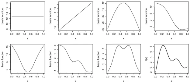
2-1 This plot (source: Wood (2006)) illustrates a rank7thin plate re gression spline basis for representing a smooth function of one variable. The first 7 panels (starting at top left) show the ba sis functions multiplied by some coefficients. These are then summed to give the smooth curve in the lower right panel. The first two bases span the space of functions that are completely smooth, according to the roughness measure defined in Section 2.3. The remaining basis functions represent the wiggly compo nent of the smooth curve. . . 9 2-2 This plot (source: Wood (2006)) illustrates a rank15thin plate re

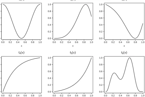
gression spline basis for representing a smooth function of two variables. The first 15 panels (starting at top left) show the ba sis functions multiplied by some coefficients. These are then summed to give the smooth surface in the lower right panel. The first three bases span the space of functions that are com pletely smooth, according to the roughness measure defined in Section 2.3. The remaining basis functions represent the wiggly component of the smooth curve. . . 10 3-1 The six test functions used in the linear predictors. . . 31

(6)

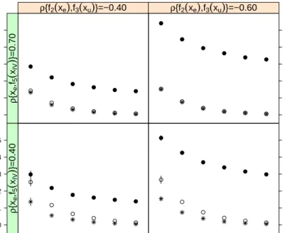
3-2 MSE results for fˆ 2(xe)when data are simulated from a Bernoulli

distribution using DGP1. Details are given in Sections 3.6.1 and 3.6.3. ◦ indicates the 2SGAM estimator results, whereas • and

∗ refer to the cases in which estimation is carried out without accounting for unmeasured confounding, and that in which the unobservable is available and included in the model. _∗ repre sents our benchmark since the right model is ﬁtted. The vertical lines show_±2standard error bands, which are only reported for the cases in which they are substantial. Notice the good overall performance of the proposed method for all sets of correlations and sample sizes. . . 34 3-3 Typical estimated smooth functions for f2(xe)(ticker solid black

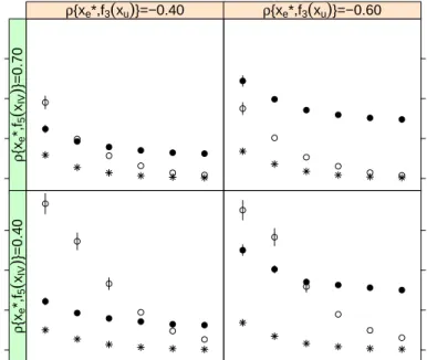
line) when employing the 2SGAM approach (black lines) and naive GAM estimation (grey lines). The dotted and solid lines indicate the results for the cases in whichn = 1000and n = 8000, respectively. Notice the convergence of the proposed method to the true function as opposed to the naive approach. . . 35 3-4 MSE results for βˆe when data are simulated from a gamma dis

tribution using DGP1. Details are given in Sections 3.6.2 and 3.6.3, and in the caption of Figure 4-3. For low sample sizes the naive method seems to outperform 2SGAM when the instru ment is not strong. See Section 3.6.4 for an explanation of this result. . . 36 3-5 Smooth function estimates of body mass index (bmi) and ξˆu on

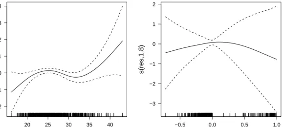
the scale of the linear predictor, for the second stage equation. Dashed lines represent 95% Bayesian conﬁdence intervals cor rected as discussed in Section 3.5. The numbers in brackets in the y-axis captions are the estimated degrees of freedom or ef fective number of parameters of the smooth curves. The rug plot, at the bottom of each graph, shows the covariate values . . 39

(7)

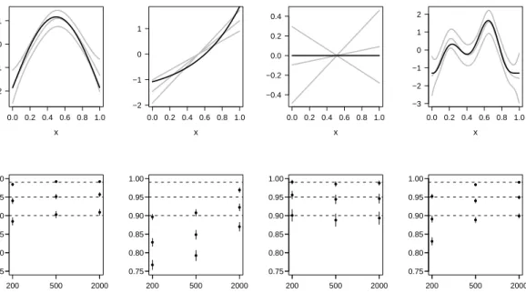
4-1 Results from component-wise Bayesian intervals for Bernoulli simulated data at three sample sizes. Observations were gener ated as logit_{E(Yi)}= α+zi+f1(x1i) +f2(x2i) +f3(x3i) +f4(x4i),

where Yi followed a bernoulli distribution and uniform covari

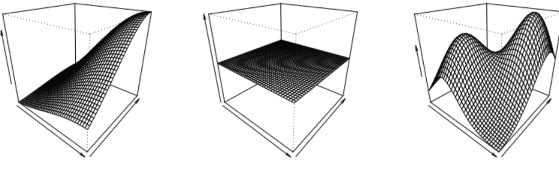
ates on the unit interval with correlations equal to 0.5 were em ployed (see section 4.3.1 for details). The function definitions are given in Table 4.1. The functions were scaled to have the same magnitude in the linear predictor and then the sum rescaled to produce probabilities in the range [0.02,0.98]. 1000 replicate datasets were then generated and GAMs fitted using penalized thin plate regression splines (Wood, 2003) with basis dimen sions equal to 10, 10, 10 and 20, respectively, and penalties based on second-order derivatives. Multiple smoothing parameter se lection was by generalized AIC (Wood, 2008). Displayed in the top row are the true functions, indicated by the black lines, as well as example estimates and 95% Bayesian confidence inter vals (gray lines) for the smooths involved. represents the mean _• coverage probability from the 1000 across-the-function coverage proportions of the intervals, vertical lines show_±2standard er ror bands for the mean coverage probabilities, and dashed hor izontal lines show the nominal coverage probabilities considered. 43 4-2 The three two-dimensional test functions used in the linear pre

dictor η2,i. . . 55

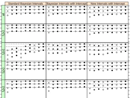
4-3 Coverage probability results for binomial data generated us ing η1,i as a linear predictor. Covariate correlation was equal

to 0.5. Details are given in section 4.3. _◦, _⊕ and _• stand for high, medium and low noise level respectively. Standard er ror bands are not reported since they are smaller than the plot ting symbols. Notice the improvement in the performance of the component-wise intervals for f2(x), when the intercept is

included in the calculations. . . 58 4-4 Coverage probability results for gamma data. Details are given

in the caption of Figure 4-3. . . . 58 4-5 Coverage probability results for Poisson data for the case in

which correlated uniform covariates were obtained setting ρ = 0. Details are given in the caption of Figure 4-3. . . 59

(8)

4-6 Coverage probability results for Poisson data for the case in which ρwas set to 0.5. Details are given in the caption of Figure 4-3. . . 59 4-7 Coverage probability results for Poisson data for the case in

which ρwas set to 0.9. Details are given in the caption of Figure 4-3. Notice how the conﬁdence interval performance for f1(x)

and f2(x)degrades when oversmoothing, due to high covariate

correlation, occurs. . . 60 4-8 Coverage probability results for Gaussian data generated using

η2,i as a linear predictor. Covariate correlation was equal to 0.5.

Details are given in the caption of Figure 4-3. Notice the im provement in the performance of the intervals forf5(x, z), when

the intercept is included in the calculations. . . 60 4-9 Smooths corresponding to 50 draws from (2.5) obtained from

ﬁtting an additive model to 200 observations generated as Yi =

f4(xi) +ǫi, where ǫi ∼ N(0, σ2)with σ = 0.3, and x is a uniform

covariate on the unit interval. The function f4 is displayed and

deﬁned in Figure 4-1 and Table 4.1, respectively. The shaded regions represent 95%Bayesian intervals from the ﬁtted model. 62 5-1 The test functions used to generate the datasets. . . 76 5-2 MSE comparisons between GCV/AIC and REML for four er

ror distributions and methods discussed in Section 5.2, when using linear predictor η1. Covariate correlation is 0 and the sig

nal to ratio level is medium. Baseline indicates that no shrink age smoother is used during the model ﬁtting process. Fur ther simulation details are given in Section 5.3.1. Boxplots show the distributions of differences in mean squared error between GCV/AIC and REML. In all cases a Wilcoxon signed rank test indicates the REML has lower MSE than GCV/AIC (p-value <

(9)

5-3 MSE results between the methods discussed in Section 5.2 and the double penalty approach for four error distributions and lin ear predictor η1. REML estimation is employed for all methods

except for GAM boosting and the Belitz&Lang approach. Co variate correlation is 0 and the signal to ratio level is medium. Baseline indicates that no shrinkage smoother is used during the model ﬁtting process. Further simulation details are given in Section 5.3.1. Boxplots show the distributions of differences in mean squared error between each method and the double penalty approach. In all cases a Wilcoxon signed rank test in dicates that double penalty has lower MSE than the competing methods (p-value < 10−6_{), except for the Backward method in}

the Gaussian and Binomial cases where there is no signiﬁcant difference (p-value > 0.10). . . 79 5-4 Shrinkage results for the methods discussed in Section 5.2, for

four error distributions and linear predictor η1. REML estima

tion is employed for all methods except for GAM boosting and the Belitz&Lang approach. Covariate correlation is 0 and H, M and L stand for high, medium and low signal level. Baseline indicates that no shrinkage smoother is used during the model ﬁtting process. Further simulation details are given in Section 5.3.1. False positive rates give the proportion of times spurious terms are selected. Vertical lines show _±2standard error bands. 80 5-5 Shrinkage results for the methods discussed in Section 5.2, for

four error distributions and linear predictor η1. REML estima

tion is employed for all methods except for GAM boosting and the Belitz&Lang approach. Covariate correlation is 0.9. Further details are given in the caption of Figure 5-4. . . 80 5-6 MSE comparisons between some of the methods discussed in

Section 5.2 and the double penalty approach for four error dis tributions, when REML estimation and linear predictor η2 are

employed. Covariate correlation is 0 and the signal to ratio level is medium. Baseline indicates that no shrinkage smoother is used during the model ﬁtting process. Further simulation de tails are given in Section 5.3.1 and in the caption of Figure 5-3. In all cases a Wilcoxon signed rank test indicates that double penalty has lower MSE than the competing methods (p-value <

(10)

5-7 Shrinkage results for some of the methods discussed in Section 5.2 and four error distributions, when REML estimation and lin ear predictor η2 are employed. Covariate correlation is 0. Fur

ther simulation details are given in Section 5.3.1 and in the cap tion of Figure 5-4. . . . 82 5-8 MSE comparisons between some of the methods discussed in

Section 5.2 and the double penalty approach for four error dis tributions and linear predictor η3. REML estimation is employed

for all methods except for GAM boosting. Models are ﬁtted us ing fourteen covariates, eleven of which are not inﬂuential. Co variate correlation is 0 and the signal to ratio level is medium. Further simulation details are given in Section 5.3.1 and in the caption of Figure 5-3. In all cases a Wilcoxon signed rank test in dicates that double penalty has lower MSE than the competing methods (p-value < 10−5_{), except for the Shrinkage approach}

where there is no signiﬁcant difference (p-value > 0.29). . . 83 5-9 MSE comparisons between some of the methods discussed in

Section 5.2 and the double penalty approach for four error dis tributions and linear predictor η3. REML estimation is employed

for all methods except for GAM boosting. Models are ﬁtted us ing thirty covariates, twenty-seven of which are spurious. Co variate correlation is 0 and the signal to ratio level is medium. Further simulation details are given in Section 5.3.1 and in the caption of Figure 5-3. In all cases a Wilcoxon signed rank test in dicates that double penalty has lower MSE than the competing methods (p-value < 10−6_{), except for the Shrinkage approach}

where there is no signiﬁcant difference (p-value > 0.33). . . 84 5-10 Smooth function estimates obtained by applying the double penalty

approach with REML estimation on the plasma beta-carotene dataset described in Section 5.4.1. The results are reported on the scale of the linear predictor. The numbers in brackets in the y-axis captions are the edf of the smooth curves. The ‘rug plot’, at the bottom of each graph, shows the covariate values. . . 85

(11)

5-11 The top boxplots report prediction risk comparisons (in units of 103_{) between GCV and REML for some of the methods dis}

cussed in Section 5.2 when using the beta-carotene dataset (see details in Section 5.4). The plots show the distributions of dif ferences in prediction risk estimate between GCV and REML, which were obtained repeating 5-fold cross validation 100 times. In all cases a Wilcoxon signed rank test indicates the REML yields lower risk estimates as compared to GCV (p-value <

10−19_{), except for Backward where this evidence is less strong}

(p-value < 0.022). The bottom boxplots report prediction risk comparisons between the four shrinkage methods used for the beta-carotene dataset and the double penalty approach, when REML estimation is employed. The plots show the distributions of differences in prediction risk estimate between each method and double penalty. In all cases a Wilcoxon signed rank test indicates that double penalty produces lower risk estimates as compared to the competing methods (p-value < 10−18_{), except}

for Shrinkage where this evidence is less strong (p-value < 0.017). 86 5-12 Smooth function estimates obtained by ﬁtting a standard GAM

with REML estimation on the plasma beta-carotene dataset de scribed in Section 5.4.1. Further details are given in the caption of Figure 5-10. . . . 87 5-13 The same smooth function estimates as those reported in Figure

5-12. The shaded regions represent 95% Bayesian conﬁdence intervals discussed in Chapter 4. . . . 88

(12)

List of Tables

3.1 Test function deﬁnitions. f1 -f6 are plotted in Figure 3-1. . . 32

3.2 Observations were generated from the appropriate distribution with true response means, laying in the speciﬁed range, ob tained by transforming the linear predictors by the inverse of the chosen link function. l, u and s/n stand for lower bound, upper bound and signal to noise ratio parameter, respectively. The linear predictor for the binomial case was scaled to pro duce probabilities in the range [0.02,0.98]; observations were then simulated from binomial distributions with denominator nbin. In the gamma case the linear predictor was scaled to have

range [0.2,3] and one value for φ used. For the Gaussian case normal random deviates with mean 0and standard deviation σ were added to the true expected values, which were then scaled to lay in [0,1]. The linear predictor of the Poisson case was scaled in order to yield true means in the interval [0.2,3]. No tice that the chosen signal to noise ratio parameters yielded low informative responses. See Section 5.3 for further details. . . 33 3.3 Across-the-function coverage probability results forfˆ 2(xe)at four

sample sizes, for the nominal level 95%, when the correlation between instrument and endogenous variable is 0.7and that be tween endogeous and unobservable equal to −0.6. 2SGAM, and AD.2SGAM stand for the proposed two-step approach with out correction for the Bayesian intervals, and the two-step ap proach with the correction described in Section 3.5, with Nb = 25

and Nd = 100. Notice the good coverage probabilities obtained

when employing the correction. . . 37 4.1 Test function deﬁnitions. f1 -f4are plotted in Figure 4-1, and f5

(13)

4.2 Observations were generated as described in Table 3.2. The lin ear predictor for the binomial case was scaled to produce prob abilities in the range [0.02,0.98]; observations were then sim ulated from binomial distributions with denominator nbin. In

the gamma case the linear predictor was scaled to have range

[0.2,3] and three levels of φused. For the Gaussian case normal random deviates with mean 0 and standard deviation σ were added to the true expected values, which were then scaled to

4.3

lay in [0,1]. The linear predictor of the Poisson case was scaled in order to yield true means in the interval [0.2, pmax]. . . . Percentage mean squared bias (b¯2∗ _{) and mean variance (}_v¯ 2∗ _{) re}

55 sults for the smooth components of GAMs ﬁtted to data simu lated from four error models at medium noise level. Covariate correlation and sample size were 0.5 and 200 (see Section 4.3 for further details). b¯2∗ _{= ¯}_b2_/_{( ¯}_b2_{+ ¯}_v2₎_∗₁₀₀_and_v¯ 2∗ _{= ¯}_b2_/_{( ¯}_b2_{+ ¯}_v2₎_∗₁₀₀_,

where b¯2_and_v¯ 2_{were calculated following the deﬁnitions in Sec}

tion 4.2, with C_i−1 = [V_fj]ii for each smooth component j. Notice

that the B < V assumption is comfortably met for all terms ex cept for f2, which is the problematic case in the ﬁrst columns of

Figures 4-3 - 4-7. . . 64 5.1 Test function deﬁnitions. f1 -f9 are plotted in Figure 5-1. . . 77

(14)

Chapter 1 Introduction

One of the main objectives of regression modelling is to model the expected value of a response variable Y as a ﬂexible function of regressors x1, . . . , xp. In

other words, the aim is to specify a function f such that

E(Y_|x1, . . . , xp) = h{f(x1, . . . , xp)},

where h( )_· is the inverse of a link function, and Y follows an exponential family distribution. Replacing f( )_· with a linear combination of some known func tions of covariates, e.g. f(x1, . . . , xp) = θ0 + �p_j₌₁θjxj, leads to a general

ized linear model (GLM; McCullagh and Nelder, 1989) which is easy to es timate and to interpret, and for which well-developed statistical frameworks are available. However, since the functional shape of any relationship is rarely known a priori and the response of interest may depend on the predictors in a complicated manner, it is more convenient to model f( )· as the sum of some unspeciﬁed smooth function of covariates, e.g. f(x1, . . . , xp) = �_jp ₌₁fj(xj),

hence giving rise to a generalized additive model (GAM; Hastie and Tibshi rani, 1990). Such a model allows for rather flexible specification of the depen dence of the response on the covariates, but this flexibility and convenience comes at the cost of new methodological problems, some of which will be the objective of this thesis.

1.1 Objectives of Thesis and Outline

This thesis deals with some aspects of penalized regression spline smoothing. We shall begin by discussing some background material and then concentrate on three issues.

(15)

First, we consider the problem of model misspecification in the GAM con text. Specifically, when unobservables are associated with included regres sors and have an impact on the response, standard estimation methods will not be valid. This means, for example, that estimation results from observa tional studies, whose aim is to evaluate the impact of a treatment of interest a response variable, will be biased and inconsistent in the presence of unmea sured confounders if these are not accounted for. One method for obtaining consistent estimates of treatment effects when dealing with linear models and GLMs is the instrumental variable (IV) approach. Fitting procedures to carry out IV analysis within the GAM context have not been developed. Following the idea first introduced by Hausman (1978, 1983), we propose a two-stage approach for IV estimation when dealing with GAMs, and a correction pro cedure for confidence intervals. We explain under which conditions the pro posed method works and illustrate its empirical validity through an extensive simulation experiment and a health study where unmeasured confounding is suspected to be present.

Second, we study the coverage properties of the Bayesian ‘confidence’ in tervals for the smooth component functions of GAMs. The intervals are the usual generalization of Wahba (1983) or Silverman (1985) intervals to the GAM component context. We present simulation evidence showing these intervals have close to nominal across-the-function frequentist coverage probabilities, except when the truth is close to a straight line/plane function. We extend Nychka’s (1988) argument for univariate smoothing splines to explain these results. The theoretical results allow us to derive alternative intervals from a purely frequentist point of view, and to explain the impact that the neglect of smoothing parameter variability has on confidence interval performance. They also suggest switching the target of inference for component-wise inter vals away from smooth components in the space of the GAM identifiability constraints.

Third, we face the problem of GAM component selection. We propose two effective methods and extend the nonnegative garrote estimator, originally in troduced by Breiman (1995), to achieve smooth term selection. The proposals avoid having to use nonparametric testing methods for which there is not a general reliable distributional theory. Moreover, variable selection is carried out in one single step as opposed to many selection procedures which involve an exhaustive search of all possible models. The empirical performance of the proposed methods is compared to that of some available techniques via an extensive simulation study. Our results show under which conditions one

(16)

method can be preferred over another, hence providing applied researchers with some practical guidelines. The procedures are also illustrated analysing data on plasma beta-carotene levels from a cross-sectional study conducted in the United States.

This thesis is based on the following papers:

• MARRA, G., RADICE, R., 2010. Penalised regression splines: theory and application to medical research. Statistical Methods in Medical Research, 19, pp. 107–125.

• MARRA, G., RADICE, R., 2012. A Flexible Instrumental Variable Ap proach. Statistical Modelling, in press.

• MARRA, G., WOOD, S. N. Coverage Properties of Conﬁdence Intervals for Generalized Additive Model Components. Submitted.

• MARRA, G., WOOD, S. N. Practical Variable Selection for Generalized Additive Models. Submitted.

(17)

Chapter 2 Generalized Additive Models: An

Overview

GAMs allow for ﬂexible functional dependence of a response variable on co variates. The aim of this chapter is to provide a brief overview of this ﬂexible class of models, based on the penalized likelihood framework with regression splines, by discussing some aspects that are relevant to this thesis.

2.1 Introduction

GAMs are becoming among the most useful and used of statistical methods. An ISI Web of Knowledge search on the keyword “generalized additive mod els” reveals over 800 articles published during the last decade in the ﬁelds of biology, ecology, economics, environmental science, epidemiology, genetics and medicine (e.g. Marra and Radice, 2011; Marra and Radice, 2010; Zanin and Marra, 2011). This approach extends traditional GLMs by allowing the deter mination of possible nonlinear effects of covariates on a response variable of interest. In other words, GLMs model the effects of predictor variables xj in

terms of a linear predictor of the form θ0+�_jθjxj, where the θj are regression

parameters, whereas GAMs replaceθ0+ �_jθjxj with, for instance, �_jfj(xj),

where the fj are unknown smooth functions of regressors. The use of smooth

terms is crucial since the functional shape of any relationship is rarely known

a priori and the response of interest may depend on the predictors in a compli cated manner.

A number of procedures can be employed for ﬁtting GAMs, some of them documented in two recent monographs (Ruppert et al., 2003; Wood, 2006), and there is ongoing research on new ones such as the likelihood-based boosting

(18)

approach (Tutz and Binder, 2006). Our investigation is not meant to be exten sive. Rather, our goal is to present some background material on the penalized likelihood based approach with regression splines since this is the framework that will be adopted throughout this thesis.

2.2 Model Structure

A GAM can be seen as a GLM with a linear predictor involving smooth func tions of covariates

g_{E(Yi)}= ηi = X ∗ iθ + f1(x1i) +f2(x2i) +f3(x3i, x4i) +. . . , (2.1)

where g( ) · is a smooth monotonic twice differentiable link function, Yi is a

univariate response variable, X∗ _i is theith _{row of}_X∗ _{, which is the model matrix}

for any strictly parametric model components, with corresponding parameter vector θ, and the fj are smooth functions of the covariates xj. The fj are subject

to identiﬁability constraints such as �_ifj(xji) = 0 ∀j. The right hand side

of (2.1) is called the linear predictor and is denoted as ηi, and the response Yi

follows an exponential family distribution whose probability density functions

are of the form _�

yϑ₋h(ϑ) �

mϑ(y) = exp + c(y, φ) , (2.2)

φ

where h( )_· and c( )_· are arbitrary functions, ϑ is the natural and φ the disper sion parameter. The mean and variance of such a distribution are E(Y) =

∂h(ϑ)/∂ϑ = µ and var(Y) = φ∂µ/∂ϑ = φV(µ), respectively, where V(µ)

denotes the variance function. Several distributions are possible within this family, such as the binomial, gamma, Gaussian and Poisson. In fact, a whole variety of outcome measures (e.g. counts, binary and skewed data) can be modelled within this model structure. In some cases, the nature of the re sponse distribution is not known, and it is only possible to specify what the relationship between the variance of the response and its mean should be. It turns out that it is possible to develop theory for ﬁtting and inference based on the notion of quasi-likelihood. Here, maximum quasi-likelihood parameter estimates can be found by the usual method used to ﬁt a GLM, described in the next section, and the classic large sample distribution of GLM parameter estimators also hold for maximum quasi-likelihood.

Model (2.1) can ﬂexibly determine the functional shape of the relationship between a response and some explanatory variables, hence avoiding the draw

(19)

backs of modelling data using parametric relationships. As an example, let us consider a group of patients from a single hospital who underwent Coro nary Artery Bypass Graft surgery. One may wish to identify the risk factors of in-hospital mortality following surgery, where the outcome of interest is Sta tus (0=alive, 1=died) and the explanatory variables associated with surgical mortality could be Age, BSA(Body Surface Area), andEjection Fraction(a mea sure of heart function summarized in the categories ‘Good’, ‘Fair’ and ‘Poor’). In order to explain the in-hospital mortality following surgery from these ex planatory variables, several model speciﬁcations can be adopted. A possibility would be to ﬁt a GLM with linear predictor given by

ηi = θ0+ θ1EFf air,i + θ2EFpoor,i + θ3Agei + θ4BSAi, (2.3)

where θ0 represents the baseline group Ejection Fraction = ‘Good’. But we

do not know whether the variables Ageand BSAenter the model linearly, and (2.3) makes the assumption of linear relationships between the two continuous variables and response. Instead, one could employ the following GAM

ηi = θ0+ θ1EFf air,i + θ2EFpoor,i + f1(Agei) +f2(BSAi).

In this way the relationship between the in-hospital mortality and the contin uous variables in the model can be determined ﬂexibly. One of main advan tages of GAMs is that residual confounding may be avoided. This is supported by the simulation study of Benedetti and Abrahamowicz (2004) which shows that the use of spline models reduces residual confounding as compared to fully parametric modelling which typically leads to biased and spurious es timated impacts of the exposure of interest, in the presence of unmodelled nonlinearities. However, when unmeasured covariates are correlated with in cluded regressors and have an impact on the response, any GAM estimation method will not be valid, no matter how reliable and computationally robust the method is. Chapter 3 addresses this issue by showing how model misspec iﬁcation can be dealt with in the GAM context.

The smooth terms can be represented using regression splines. In particu lar, the regression spline of a predictor is made up of a linear combination of known basis functions, bjk(xj), and unknown regression parameters, βjk,

qj

fj(xj) =

�

βjkbjk(xj), (2.4) k=1

(20)

where j indicates the smooth term for the jth _{explanatory variable,} _q

j is the

number of basis functions, hence regression parameters, used to represent the jth _{smooth term, and the subscript}_i_{is dropped for simplicity. Similarly, the re}

gression spline of two covariates can be written asfjp(xj, xp) = �_kqj₌₁βjp,kbjp,k(xj, xp).

As mentioned earlier on, in order to identify (2.1), each smooth component is subject to some identiﬁability constraint. Basis functions have to be chosen in order to come up with smooth component estimates. For instance, suppose that f1(Age)is believed to be a 3th order polynomial. A basis for this space is

b11(Age) = 1, b12(Age) = Age, b13(Age) = Age2 and b14(Age) = Age3. Here,

expression (2.4) becomes

4

f1(Age) =

�

β1kb1k(Age) = β11+ β12Age + β13Age2+ β14Age3,

k=1

which can be easily estimated using standard regression techniques. The num ber of basis functions,qj, determines the maximum possible ﬂexibility allowed

for a smooth term. For example, a qj equal to 20 will yield a “wigglier” non

linear estimate as compared to the estimate that can be obtained when this parameter is set to 10. It is worth observing that, although quite illustrative, polynomial bases are not very useful in practice. As the number of basis func tions increases, polynomial bases become increasingly collinear. This yields highly correlated parameter estimators, hence leading to high estimator vari ance and numerical problems (e.g. Royston, 2005). For these reasons, such basis functions should not generally be employed to model nonlinear relation ships. As a practical solution, in some applied work, continuous variables are categorized into groups based on intervals or frequencies. However, catego rization has several disadvantages since it introduces the problem of deﬁning cut-points and implies that the relationship between a response variable and a set of covariates is ﬂat within intervals (Royston and Altman, 1994; Johansen

et al., 2005). To overcome all these issues, spline bases are typically used to determine ﬂexibly the relationship between the continuous predictors and the outcome of interest. In fact, they avoid the disadvantages of categorization, are not as correlated as polynomial basis functions, have convenient mathemati cal properties and good numerical stability. Common choices for representing smooth functions include smoothing splines (e.g. Hastie and Tibshirani, 1990; Wahba, 1990). These place knots at every data point, and are indeed some times referred to as full rank smoothers because the size of the spline basis is equal to the number of observations. However, such smoothers have as many

(21)

0 5 10 15 basis function −4 0 2 4 6 8 basis function −5 −4 −3 −2 −1 basis function −2 0 2 4 6 8 f(x) basis function 8 10 12 14 16 18 basis function −15 −5 5 10 basis function −30 −25 −20 −15 −10 basis function −5 0 5 10

unknown parameters as there are data which results in expensive computa tions. The thin plate regression spline basis proposed by Wood (2003) is a valid alternative. This basis is a low rank eigen-approximation version of the full rank thin plate spline introduced by Duchon (1977). It represents a general solution to the problem of estimating efﬁciently, and without having to choose knot locations, a smooth function of multiple predictor variables from noisy observations of the function, at particular values of those predictors. Figures 2-1 and 2-2 illustrate thin plate regression spline bases in one dimension and two dimensions, respectively. Full mathematical details can be found in Wood (2003, 2006). This spline basis will be used throughout this thesis.

0.0 0.2 0.4 0.6 0.8 1.0 0.0 0.2 0.4 0.6 0.8 1.0 0.0 0.2 0.4 0.6 0.8 1.0 0.0 0.2 0.4 0.6 0.8 1.0

x x x x

0.0 0.2 0.4 0.6 0.8 1.0 0.0 0.2 0.4 0.6 0.8 1.0 0.0 0.2 0.4 0.6 0.8 1.0 0.0 0.2 0.4 0.6 0.8 1.0

x x x x

Figure 2-1: This plot (source: Wood (2006)) illustrates a rank 7 thin plate regression spline

basis for representing a smooth function of one variable. The first 7 panels (starting at top left) show the basis functions multiplied by some coefficients. These are then summed to give the smooth curve in the lower right panel. The first two bases span the space of functions that are completely smooth, according to the roughness measure defined in Section 2.3. The remaining basis functions represent the wiggly component of the smooth curve.

2.3 Some Model Fitting Details

Given a vector of n independent observations, where Yi ∼ mϑi(yi), the substi

tution of the terms fj(xj)with their regression spline expression into a model

equation like (2.1) yields a GLM, which can be estimated by maximum likeli hood. Speciﬁcally, ηi can be rewritten as Xiβ, where Xi includes X∗ i and the

terms representing the spline bases for the fj, while β contains θ and all the

smooth coefﬁcient vectors, βj. mϑi(yi) denotes an exponential family distri

bution with probability density function (2.2) for which h and c are ﬁxed and depend on the chosen distribution. The natural parameter ϑi is determined by

(22)

z x z x z x z x

f

Figure 2-2: This plot (source: Wood (2006)) illustrates a rank 15 thin plate regression spline

basis for representing a smooth function of two variables. The first 15 panels (starting at top left) show the basis functions multiplied by some coefficients. These are then summed to give the smooth surface in the lower right panel. The first three bases span the space of functions that are completely smooth, according to the roughness measure defined in Section 2.3. The remaining basis functions represent the wiggly component of the smooth curve.

(23)

µi via E(Yi)and hence ultimately by β. The dispersion parameter φcan either

be ﬁxed or estimated, depending on the chosen distribution. For example, for the binomial and Poisson cases, φis known and equal to 1.

Since the Yi are assumed to be independent, the likelihood of β is n

L(β) = �mϑi(yi) i=1

and its log-likelihood is

n

� �_y_i_ϑ_i₋_h₍_ϑ_i₎ � l(β) = + c(yi, φ) ,

φ

i=1

where β enters the right-hand side through the ϑi. Log-likelihood maximiza

tion is achieved by partially differentiating l with respect to each element of

β setting the resulting equations to zero, and solving for β. In formulae, the maximum likelihood estimate of β satisﬁes the score equations

n n ∂l 1 � ∂ 1 �(yi −µi)�∂µi� xji � = 0 _∀j, = = ∂βj φ ∂βj { yiϑi −h(ϑi)} φ � V(µi) ∂ηi i=1 i=1

whose solution does not depend on φ. These equations can not be solved alge braically, hence a numerical iterative procedure has to be employed. In prac tice, the likelihood can be maximized by Iteratively Re-Weighted Least Squares (IRLS), where the GLM is ﬁtted by iterative minimization of the problem

[k] 2

�√W[k]₍_z ₋_X_β₎_� _w.r.t. _β_.

k is the iteration index, z[k] = Xβ[k]+ G[k](y ₋µ[k]), µ[i k] is the current model estimate of E(Yi), G[k]is a diagonal matrix such that G[ii

k]

= g ′ ₍_µ[

i k]

), and W[k]

is a diagonal matrix given by W_ii[k] = [G_ii[k]2V(µ_i[k])]−1_{. To avoid overﬁtting it}

is necessary to fit the model by penalized maximum likelihood estimation in which roughness measures are used to control overfit. For the case of smooth functions of one variable, the penalized likelihood is maximized by penalized IRLS (P-IRLS), so that the GAM is fitted by iteratively minimizing the problem

�√W[k]₍_z[k] −Xβ)_�2+ �λj � � f_jdj (xj) �2 dxj w.r.t. β. j

The terms in the summation measure the roughness of the smooth functions, dj (usually set to 2) indicates the order of the derivatives for the jth smooth

(24)

term to be used in the ﬁtting process, and the λj are smoothing parameters

that control the trade-off between ﬁt and smoothness. Since regression splines

dj

are linear in their model parameters, the penalty �_jλj

� �

f_j (xj)

�2

dxj can be

written as a quadratic form in β with known coefﬁcient matrices S_j. As an example, by setting dj = 2 and for a regression spline basis in one dimension,

we have that � � f_j2(xj) �2 dxj = � � ∂2_f j(xj)�2 dxj = � � ∂2� k qj =1βjkbjk(xj) �2 dxj ∂x2 _∂x2 j j = � �βTb_j′′ (xj) �2 dxj = � βTb_j′′ (xj)bj′′ (xj)Tβdxj = βT �� b_j′′ (xj)bj′′ (xj)Tdxj � β = βTSjβ,

where b ′′ _j(xj) is a vector containing the second derivatives of the basis func

tions for the jth _{smooth term with respect to}_x

j. It follows that � λj � � f_jdj (xj) �2 dxj = � λjβTSjβ. j j

The precise mathematical expression of a thin regression spline basis and its penalty depends on the value of dj and the dimension of xj; see Wood (2003,

2006) for full mathematical details. The smoothing parameters play a crucial role in penalized regression spline estimation: very large values for λj lead

to very smooth estimates and vice versa. Given smoothing parameters, the penalized nonlinear least squares problem can be solved by using the IRLS algorithm. It turns out that the form of the parameter estimators of β is

βˆ = (XTWX+ S)−1XTWz,

where S = �_jλjSj. It follows that the estimator for β is biased because of

penalty-induced bias.

Smoothing parameter estimation has to be addressed as well. This can be achieved by minimization of a prediction error estimate, such as the gener alized cross validation (GCV) score, if a dispersion parameter has to be es timated, or the generalized Akaike’s information criterion (AIC). Following Wood (2008), smoothing parameter selection via the GCV score consists of minimizing

nD(βˆ)

Vg(λ) = ,

(25)

where D(βˆ), the model deviance, is deﬁned as 2φ(ˆlsat −lˆ(βˆ)), ˆl(βˆ)is the log

likelihood of the ﬁtted model andˆlsat the maximum value for the log-likelihood

of the model with one parameter per datum. The matrix Ais given byWX(XT_WX₊

S)−1_XT_W_{, and the}_λ

j enter the GCV score through A. In case φ is known, the

following generalized AIC is minimized instead

Va(λ) = D(βˆ) + 2tr(A)φ.

As an alternative, REML can be employed. Within this framework, the pe nalized likelihood estimates, βˆ, can be seen as the posterior modes of the dis tribution of β_|y if β _∼ N(0,S−φ), where S− is an appropriate generalized inverse. Viewing the spline parameters as random effects allows for the pos sibility to estimate the λi via REML (Wahba, 1985). Wahba (1985) showed

that asymptotically prediction error criteria are better in a mean square er ror sense, even though H¨ardle et al. (1988) pointed out that these criteria give slow convergence to the optimal smoothing parameters. The recent work by Reiss and Ogden (2009) shows that at ﬁnite sample sizes GCV or AIC is prone to undersmoothing and is more likely to develop multiple minima than REML (e.g. Wood, 2010). So, it would appear that REML should be preferred over GCV/AIC especially when the primary purpose of the analysis is to carry out smooth component selection. The computational methods for automatic smoothing parameter estimation of Wood (2006, 2008, 2010) are based on the criteria mentioned above, and will be used throughout this thesis.

2.4 Conﬁdence Intervals

The well known Bayesian ‘conﬁdence’ intervals originally proposed by Wahba (1983) or Silverman (1985) in the univariate spline model context, and then generalized to the component-wise case when dealing with GAMs (e.g. Gu, 1992; Gu, 2002; Gu and Wahba, 1993; Wood, 2006), are typically used to reli ably represent the uncertainty of smooth terms. This is because such intervals include both a bias and variance component (Nychka, 1988), a fact that makes these intervals have good observed frequentistcoverage probabilities across the function.

The large sample posterior used for interval calculations is given by

(26)

�

where βˆis the maximum penalized likelihood estimate of β, Vβ = (XTWX+

S)−1_{φ, and}_W_and_z_{are the diagonal weight matrix and the pseudodata vector}

at convergence of the P-IRLS algorithm. Notice that W and φ are equal to the identity matrix and σ2_{, respectively, when a normal response is assumed and}

an identity link function selected; furthermore, in the normal errors case, the result above holds independently of asymptotic arguments.

In Chapter 4, we study the coverage properties of these intervals. Specif ically, we present simulation evidence showing these intervals have close to nominal across-the-function frequentist coverage probabilities, and extend Ny chka’s (1988) argument for univariate smoothing splines to the GAM compo nent case to explain these results.

2.5 Testing for No Effect

In order to achieve component selection, a number of hypothesis testing ap proaches have been proposed in the literature, each of them with advantages and disadvantages. Here, we follow the approach by Wood (2006).

Asymptotic arguments for maximum likelihood estimators suggest that if a model is correctly speciﬁed, then in the large sample limit

βˆ_∽N �E(βˆ),V_βˆ

� ,

where E(βˆ) = β because of penalty-induced bias, and the frequentist covari ance matrix is given by

V(βˆ) = V�(XTWX+ S)−1XTWz�

= (XTWX+ S)−1XTWV(z)WX(XTWX+ S)−1

= BV(η + G(y₋µ))BT= BV(Gy)BT = BGV(y)GTBT,

where B = (XT_WX₊_S₎−1_XT_W_{, and}_V₍_y₎_{is a diagonal matrix with elements} �

∂ηi

Vii = V(µi)φ. Recalling that G is a diagonal matrix such that Gii = _∂µ_i

� , it follows that GV(y)GT ₌_W−1_φ_{and therefore that}

V_βˆ = (XTWX+ S)−1XTWX(XTWX+ S)−1φ.

The dispersion parameter φ can be estimated by the Pearson estimator φˆ =

�√W(y ₋µˆ)_�2_/_{_n₋_tr₍_A₎_}_{, where}_µ_{ˆ =} _Ay_{. The trace of} _A _{represents the}

(27)

degree of complexity or number of effective parameters in the model. The edf of the model is given by the sum of the edf of the smooth functions. For the case of a smooth function of one covariate with dj = 2, if edfj = 1then it means

that the explanatory variable xj can enter the model linearly.

The parameter estimators ofθ are unpenalized. This means that classic dis tributional results for GLMs can be used for parametric terms. In particular, hypothesis testing and conﬁdence intervals can be based on the Gaussian or an appropriate t distribution, depending on whether φ is known. As for the penalized regression spline parameter estimators, given that E(βˆ_j) =_� β_j, the usual distributional results for GLMs can not be employed for hypothesis test ing. However, when the goal of the analysis is testing that a smooth term of a GAM is equal to zero, we have that if βj = 0 then E(βˆj) ≈ 0 (Wood, 2006). It

follows that, under the null hypothesis that the coefﬁcients of a smooth com ponent are zero,

ˆ T βˆ_jVr− βjβj∽˙χr 2 ˆ _, ˆ

where r denotes the rank of the covariance matrix of βˆ_j, and Vr−

βj is the rank

r generalized pseudoinverse ofV_βˆ_j that has to be employed to overcome pos

sible matrix rank deﬁciencies deriving from the fact that the smoothing penalty may suppress some dimensions of the parameter space. r is determined heuris tically as follows. It is the minimum value between the maximum edf value allowed for the jth _{smooth term (which is also the number of basis functions}

used for the term) and the smallest integer not less than the quantity calcu lated as 2_∗edfj (Wood, 2006). Ifφis unknown, then the null hypothesis can be

tested using the following result

ˆ T βˆ_jVr_β−βˆ_j/r j = βˆ Vˆr_ˆ− ˆ βj T _β j/r∽˙Fr,n−edf, j ˆ φ/φ

since Vˆ_βˆ_j is based on φˆ. As pointed out in Wood (2006), these two p-value

deﬁnitions are only approximate and one has to be careful when using these results for variable selection purposes.

Despite the fact that some testing methods have been introduced in the GAM context, such as the one discussed in this section, a general reliable dis tributional theory for the smooth terms of a GAM has not been developed to date. In Chapter 5, we tackle this problem and propose three practical methods to achieve GAM component selection.

(28)

� �

2.6 Model Comparison

In any model building process, the researcher might be interested in compar ing two nested models. Nesting implies that the simpler model (H0) is a special

case of the more complex model (H1). For example, the explanatory variables

present in H0are a subset of those present in H1. In such cases, the generalized

likelihood ratio test is often applied. Speciﬁcally, consider testing H0 : X0β0 against H1 : Xβ,

where X0 ⊂X. If H0is true then in the large sample limit

D0−D1 ∽χ2edf1−edf0,

where D0 and D1 are the deviances under H0 and H1, respectively. When a

dispersion parameter has to be estimated the F-ratio test may be used F = (D0−D1)/(edf1−edf0) ∽˙Fedf1−edf0,n−edf1 ,

D1/(n −edf1)

which does not require knowledge of φ(Wood, 2006).

2.7 Model Checking

Before interpreting model results and for model comparison purposes, the ad equacy of the ﬁtted models has to be checked. This is perhaps the most im portant part of any statistical analysis since unexplained systematic structure in the residuals of a ﬁtted model typically leads to misleading inferences.

Model checking for GAMs, which is similar to what is done for linear mod els and GLMs, can be performed using Pearson or deviance residuals (McCul lagh and Nelder, 1989). The Pearson residual has the form

(P) Yi −µˆi

r_i = ,

var(Yi)

where µˆi and varˆ (Yi) are the ﬁtted mean and variance for the ith observation

in the dataset. Under the assumption that the ﬁtted model is correct, the Pear son residuals have approximately zero mean and standard deviation close to

1. However, as discussed in Cameron and Trivedi (1998), these residuals are generally asymmetrically distributed. As an alternative, one can use deviance

(29)

residuals since they can suggest which observations cause lack of ﬁt, and are expected to behave something like standard normal random variables. The deviance residual is deﬁned as

(d)

ri = sign(Yi −µˆi)√ci,

where ci represents the contribution of the ith observation to the overall good

(30)

Chapter 3 A Flexible Instrumental Variable

Approach

Classical regression model literature has sometimes assumed that measured and unmeasured or unobservable covariates are statistically independent. For many applications this assumption is clearly tenuous. When unobservables are associated with included regressors and have an impact on the response, standard estimation methods will not be valid. This means, for example, that estimation results from observational studies, whose aim is to evaluate the im pact of a treatment of interest on a response variable, will be biased and incon sistent in the presence of unmeasured confounders. One method for obtaining consistent estimates of treatment effects when dealing with linear models is the instrumental variable (IV) approach. Linear models have been extended to GLMs and GAMs, and although IV methods have been proposed to deal with GLMs, ﬁtting methods to carry out IV analysis within the GAM context have not been developed. We propose a two-stage procedure for IV estimation when dealing with GAMs represented using any penalized regression spline approach, and a correction procedure for conﬁdence intervals. We explain un der which conditions the proposed method works and illustrate its empirical validity through an extensive simulation experiment and a health study where unmeasured confounding is suspected to be present.

3.1 Introduction

Observational data are often used in statistical analysis to infer the effects of one or more predictors of interest (which can be also referred to as treatments) on a response variable. The main characteristic of observational studies is a

(31)

lack of treatment randomization which usually leads to selection bias. In a re gression context, the most common solution to this problem is to account for confounding variables that are associated with both treatments and response (e.g. Becher, 1992). However, the researcher might fail to adjust for pertinent confounders as they might be either unknown or not readily quantiﬁable. This constitutes a serious limitation to covariate adjustment since the use of stan dard estimators typically yields biased and inconsistent estimates. Hence, a major concern when estimating treatment effects is how to account for unmea sured confounders.

This problem is known in econometrics as endogeneity of the predictors of interest. The most commonly used econometric method to model data that are affected by the unobservable confounding issue is the instrumental vari able (IV) approach (Wooldridge, 2002). This technique only recently has re ceived some attention in the applied statistical literature. This method can yield consistent parameter estimates and can be used in any kind of analysis in which unmeasured confounding is suspected to be present (e.g. Beck et al., 2003; Leigh and Schembri, 2004; Linden and Adams, 2006; Wooldridge, 2002). The IV approach can be thought of as a means to achieve pseudo randomiza tion in observational studies (Frosini, 2006). It relies on the existence of one or more IVs that induce substantial variation in the endogenous/treatment variables, are independent of unobservables, and are independent of the re sponse conditional on all measured and unmeasured confounders. Provided that such variables are available, IV regression analysis can split the variation in the endogenous predictors into two parts, one of which is associated with the unmeasured confounders (Wooldridge, 2002). This fact can then be used to obtain consistent estimates of the effects of the variables of interest.

The applied and theoretical literature on the use of IVs in parametric and nonparametric regression models with Gaussian response is large and well understood (Ai and Chen, 2003; Das, 2005; Hall and Horowitz, 2005; Newey and Powell, 2003). In many applications, however, Gaussian regression mod els have been replaced by GLMs and GAMs (McCullagh and Nelder, 1989; Hastie and Tibshirani, 1990), as they allow researchers to model data using the response variable distribution which best ﬁts the features of the outcome of interest, and to make use of nonparametric smoothers since the functional shape of any relationship is rarely known a priori. Simultaneous maximum likelihood estimation methods for GLMs in which selection bias is suspected to be present have been proposed. Here consistent and efﬁcient estimates can be obtained by jointly modelling the distribution of the response and the endoge

(32)

nous variables (Heckman, 1978; Maddala, 1983; Wooldridge, 2002). However, the main drawbacks are typically computational cost and the derivation of the joint distribution, issues that may become more severe in the GAM context. Amemiya (1974) proposed an IV generalized method of moments (GMM) ap proach to consistently estimate the parameters of a GLM. An epidemiological example is provided by Johnston et al. (2008). Here it is not clear how such an approach can be implemented for GAMs so that reliable smooth component estimates can be obtained in practice. This is because when ﬁtting a GAM the amount of smoothing for the smooth components in the model has to be se lected with a certain degree of precision. In this respect, it might be difﬁcult to develop a reliable computational multiple smoothing parameter method by taking an IV GMM approach, and, to the best of our knowledge, such a proce dure has not been developed to date.

The IV extension to the GAM context is a topic under construction. This generalization is important because even if we use an IV approach to account for unmeasured confounders, we can still obtain biased estimates if the func tional relationship between predictors and outcome is not modelled flexibly. The aim of this chapter is to extend the IV approach to GAMs by exploiting the two-stage procedure idea first proposed by Hausman (1978, 1983) and em ploying one of the reliable smoothing approaches available in the GAM lit erature. To simplify matters, we first discuss a two-step estimator for GLMs which can be then easily extended to GAMs. The proposed approach can be efficiently implemented using some standard existing software. Our proposal is illustrated through an extensive simulation study and in the context of a health study.

The rest of the chapter is structured as follows. Section 3.2 discusses the IV properties, the classical two-stage least squares (2SLS) method, and the Haus man’s endogeneity testing approach. For simplicity of exposition, Section 3.3 illustrates the main ideas using GLMs, which are then extended to the GAM context in Section 3.4. Section 3.5 proposes a conﬁdence interval correction procedure for the two-stage approach of Section 3.4. Section 3.6 evaluates the empirical properties of the two-step GAM estimator through an extensive sim ulation experiment, whereas Section 3.7 illustrates the method via a health ob servational study of medical care utilization where unmeasured confounding is suspected to be present.

(33)

3.2 Preliminaries and motivation

In empirical studies, endogeneity typically arises in three ways: omitted vari ables, measurement error, and simultaneity (see Wooldridge (2002, p. 50) for more details on these forms of endogeneity). Here, we approach the problem of endogenous explanatory variables from an omitted variables perspective.

To ﬁx ideas, let us consider the model

Y = β0+ βeXe + βoXo + βuXu + ǫY , E(ǫY |Xe, Xo, Xu) = 0, (3.1)

where ǫY is an error term normally distributed with mean 0and constant vari

ance, β0 represents the intercept of the model, and Xe, Xo and Xu are the en

dogenous variable, observable confounder, and unmeasured confounder, with parameters βe, βo and βu, respectively. We assume that Xu inﬂuences the re

sponse variable Y and is associated with Xe.

Since Xu can not be observed, (3.1) can be written as

Y = β0 + βeXe + βoXo + ζ, (3.2)

where ζ = βuXu + ǫY . OLS estimation of equation (3.2) results in inconsistent

estimators of all the parameters, with βe generally the most affected. In order

to obtain consistent parameter estimates, an IV approach can be employed. Speciﬁcally, to clear up the endogeneity of Xe, we need an observable variable

XIV , called instrument or IV, that satisﬁes three conditions (e.g. Greenland,

2000):

1. The ﬁrst requirement can be better understood by making use of the fol lowing model

Xe = α0+ αoXo + αIV XIV + αuXu + ǫXe, (3.3)

where ǫXe has the same features asǫY . (3.3) can also be written as

Xe = α0+ αoXo + αIV XIV + ξu, E(ξu|Xo, XIV ) = 0,

where ξu, deﬁned as αuXu + ǫXe , is assumed to be uncorrelated with Xo

and XIV , and αIV must be signiﬁcantly different from 0. In other words,

XIV must be associated with Xe conditional on the remaining covariates

in the model.

(34)

the other regressors in the model and Xu.

3. The third condition requires XIV to be independent of Xu.

As an example, let us consider the study by Leigh and Schembri (2004). The aim of their analysis was to estimate the effect of smoking on physical functional status. Smoking was considered as an endogenous variable since it was assumed to be associated with health risk factors which could not be observed. The IV was cigarette price as it was believed to be logically and statistically associated with smoking, and not to be directly related to any in dividual’s health. Also, it was logically assumed to be unrelated to those un measured health risk confounders which could affect physical functional sta tus. Cigarette price therefore appeared to satisfy the conditions for a valid and strong instrument. In many situations identification of a valid instrument is less clear than in the case above, and is usually heavily dependent on the spe cific problem at hand. This is because some of the necessary assumptions can not be verified empirically, hence the selection of an instrument has to be based on subject-matter knowledge, not statistical testing. Assuming that an appro priate instrument can be found, several methods can be employed to correctly quantify the impact that a predictor of interest has on the response variable, 2SLS being the most common.

In 2SLS estimation, least squares regression is applied twice. Specifically, the first stage involves fitting a linear regression of Xe on Xo and XIV to obtain Eˆ(Xe|Xo, XIV ) or Xê. In the second stage, a regression of Y on Xê and Xo

is performed. We see why this procedure yields consistent estimates of the parameters by taking the conditional expectation of (3.2) given Xo and XIV .

That is,

E(Y_|Xo, XIV ) = β0+ βeXˆe + βoXo.

Thus, the 2SLS estimator can produce an estimate of the original parameter of interest. However, this approach does not yield consistent estimates of the coefficients when dealing with generalized models (Amemiya, 1974). This is because the unobservable is not additively separable from the systematic part of the model. The following argument better explains this point. 2SLS implies the replacement of βeXe with βe(Xê + ξû). Thus, the error of model (3.2) is

allowed to become (βeξˆu + βuXu + ǫY ), which can be readily shown to be un

correlated with Xˆe and Xo. This result does not hold for GLMs because βeξˆu

and βuXu can not become part of the error term given the presence of a link