ROLLINS III, JONATHAN DARRELL, Ph.D. A Comparison of Observed Score Approaches to Detecting Differential Item Functioning among Multiple Groups. (2018) Directed by Dr. Richard M. Luecht and Dr. John T. Willse. 138 pp.
The overall purpose of this dissertation was to compare various observed score approaches in detecting differential item functioning among multiple examinee groups simultaneously. Specifically, this study contributes to the literature base by investigating a lasso-constraint observed score method (i.e., logistic regression lasso; LR lasso) in the context of multiple groups as well as features of test design related to test information targets. Given that a lasso-constraint method has not been extended for multiple groups using observed scores, comparisons are made with other observed score techniques (i.e., generalized Mantel-Haenszel χ2 and generalized logistic regression) while using item response theory to generate data (thus avoiding model-data congruity complications in the study design).
Multiple variables were manipulated in a simulation study at the test-level (e.g., the location of the test information target relative to the central tendency of the examinee population, and the shape of the test information function), item-level (e.g., the location of DIF items relative to the test information target, and the percentage of DIF items), and for simulees (e.g., the amount of impact and sample size balance). The relative lack of literature which explores DIF as it relates to target test information functions provided the exigency for exploring it within this study, along with its typical absence in literature using IRT generation models. Practitioners may find the results useful in judging the merit of adopting the newer lasso method for detecting DIF within multiple groups as opposed to pre-existing methods. Furthermore, the test design features of this study allow
for the interpretation to be less theoretical in nature and better aligned with standard operational practices, such as building exams to be optimized at test information targets, for example.
The results provide consilience that the LR lasso method has inflated type I error overall with no additional benefit in power. In fact, even when type I error rates are comparable across methods, LR lasso has a lower hit rate in many instances (i.e., higher type II error rate). The sensitivity of LR lasso to detecting DIF items seems to be
substantially influenced by having an increased number of DIF items on a form. Recommendations for practitioners, as well as limitations and directions for future research, are provided as well.
Taken collectively, the results of the simulation study can be interpreted to support the claim that LR lasso fails to perform comparably with more established methods for multiple groups DIF detection across numerous instances but could
potentially have merit in practical application in situations that have yet to be explored. While some limitations of LR lasso were noted within this study, there are a variety of other conditions which need to be explored before practitioners discard the method altogether (a few such studies are suggested). It may well be the case that the added complexity afforded by the regularization in estimating the group-specific model parameters through lasso constraints may confound the detection of the DIF items.
A COMPARISON OF OBSERVED SCORE APPROACHES TO DETECTING DIFFERENTIAL ITEM FUNCTIONING AMONG MULTIPLE GROUPS
by
Jonathan Darrell Rollins III
A Dissertation Submitted to the Faculty of The Graduate School at The University of North Carolina at Greensboro
in Partial Fulfillment
of the Requirements for the Degree Doctor of Philosophy Greensboro 2018 Approved by ______________________________ Committee Co-Chair ______________________________ Committee Co-Chair
ii
APPROVAL PAGE
This dissertation written by JONATHAN DARRELL ROLLINS III has been approved by the following committee of the Faculty of The Graduate School at The University of North Carolina at Greensboro.
Committee Co-Chairs ________________________________________ Dr. Richard M. Luecht ________________________________________ Dr. John T. Willse Committee Members ________________________________________ Dr. Randall Penfield ________________________________________ Dr. Devdass Sunnassee ____________________________ Date of Acceptance by Committee _________________________ Date of Final Oral Examination
iii
ACKNOWLEDGEMENTS
It is with great gratitude and humility that I give thanks in successfully reaching this milestone in my life. Above everything else, God is given all sovereignty and glory. I love both of my parents and brother with the ever-constant support and unconditional love that they have shown me throughout my life. None of this dissertation would have been remotely possible without them. Close friends and family at every step in my education have been such a positive support, and largely have held a role in my progress up to this point.
Without the help of my committee members, a great portion of my knowledge and this dissertation would not exist. My committee co-chairs, Dr. Luecht and Dr. Willse, have had an absolutely pivotal impact on my knowledge and skills that will stay with me for a lifetime. I cannot express enough gratitude for their unwavering support and
suggestions during this process, as well as throughout my time in graduate school and as I start my career. They inspire me to strive for greatness. Also, I would like to thank Dr. Sunnassee for his guidance and support. He has had a significant impact on how I approach many challenges and on how I reflect on my progress. I am indebted to Dr. Penfield for his encouragement and suggestions, as well as his influence on many of my current research interests.
Additionally, I would like to underscore the importance of the rest of the ERM faculty with whom I took coursework and collaborated on projects, and Dr. Ackerman, Dr. Chalhoub-Deville, Dr. Downs, and Dr. Henson. All my professors, as well as my
iv
experiences with Winston-Salem / Forsyth County Schools, the College Entrance
Examination Board, and the Georgia Department of Education molded me as a scholar. It would be remiss of me not to give thanks to the rest of the educators throughout my entire life in giving me knowledge and help in reaching this point.
v
TABLE OF CONTENTS
Page
LIST OF TABLES ... vii
LIST OF FIGURES ... ix
CHAPTER I. INTRODUCTION ... 1
Background of the Problem ... 1
Purpose and Rationale ... 11
Research Questions and Study Variables ... 13
Definition of Key Terms and Notation ... 15
Study Organization ... 15
II. LITERATURE REVIEW ... 17
Overview of Observed Score Multiple Groups DIF Methods ... 17
Item Response Theory and Dichotomous Data ... 33
Person Characteristics ... 38
III. DATA AND METHODOLOGY ... 42
Simulation Design and Conditions ... 42
Data Generation ... 44
Evaluation of Results ... 55
IV. RESULTS ... 59
Research Question One ... 59
Research Question Two ... 74
V. DISCUSSION ... 89 Test-Level Characteristics ... 89 Item-Level Characteristics ... 90 Simulee Characteristics ... 92 Practical Scenarios ... 94 Recommendations ... 103
Considerations of Effect Size Measures ... 104
vi
Conclusion ... 109 REFERENCES ... 112
vii
LIST OF TABLES
Page Table 1. List of Selected Terms and Notation Along with Brief Definitions ... 16 Table 2. Comparison of LR Model Parameters for the Three Null Hypotheses
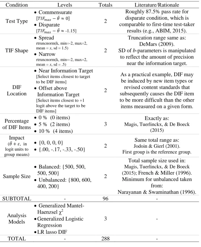
Tested in the Likelihood Ratio Test. ... 28 Table 3. Summary of Simulation Conditions Including the List and Count of
Levels for Each Condition. ... 45 Table 4. Correct Classification Rates (as Percentages) for Commensurate Test
Targets and No Simulee Impact. ... 61 Table 5. Correct Classification Rates (as Percentages) for Commensurate Test
Targets and a Half Logit Total of Simulee Impact. ... 61 Table 6. Correct Classification Rates (as Percentages) for Disparate Test Targets
and No Simulee Impact. ... 62 Table 7. Correct Classification Rates (as Percentages) for Disparate Test Targets
and a Half Logit Total of Simulee Impact. ... 63 Table 8. Type I Error Rates (as Percentages) for Commensurate Test Targets and
No Simulee Impact. ... 64 Table 9. Type I Error Rates (as Percentages) for Commensurate Test Targets and
a Half Logit Total of Simulee Impact. ... 65 Table 10. Type I Error Rates (as Percentages) for Disparate Test Targets and No
Simulee Impact. ... 67 Table 11. Type I Error Rates (as Percentages) for Disparate Test Targets and a
Half Logit Total of Simulee Impact. ... 67 Table 12. Hit Rates (as Percentages) for Commensurate Test Targets and No
Simulee Impact. ... 68 Table 13. Hit Rates (as Percentages) for Commensurate Test Targets and a Half
viii
Table 14. Hit Rates (as Percentages) for Disparate Test Targets and No
Simulee Impact. ... 70
Table 15. Hit Rates (as Percentages) for Disparate Test Targets and a Half Logit Total of Simulee Impact. ... 70
Table 16. Phi Correlations of Predicted and Truth for Commensurate Test Targets and No Simulee Impact. ... 72
Table 17. Phi Correlations of Predicted and Truth for Commensurate Test Targets and a Half Logit Total of Simulee Impact. ... 72
Table 18. Phi Correlations of Predicted and Truth for Disparate Test Targets and No Simulee Impact. ... 73
Table 19. Phi Correlations of Predicted and Truth for Disparate Test Targets and a Half Logit Total of Simulee Impact. ... 73
Table 20. Agreement Measures for Correct Classification Rates among Methods across All Conditions and Replications. ... 74
Table 21. Specification of Condition Levels for Scenario One. ... 95
Table 22. Simulation Results across 500 Replications for Scenario One. ... 95
Table 23. Specification of Condition Levels for Scenario Two. ... 96
Table 24. Simulation Results across 500 Replications for Scenario Two. ... 96
Table 25. Specification of Condition Levels for Scenario Three. ... 98
Table 26. Simulation Results across 250 Replications for Scenario Three. ... 98
Table 27. Specification of Condition Levels for Scenario Four. ... 100
Table 28. Simulation Results across 250 Replications for Scenario Four. ... 100
Table 29. Specification of Condition Levels for Scenario Five... 102
ix
LIST OF FIGURES
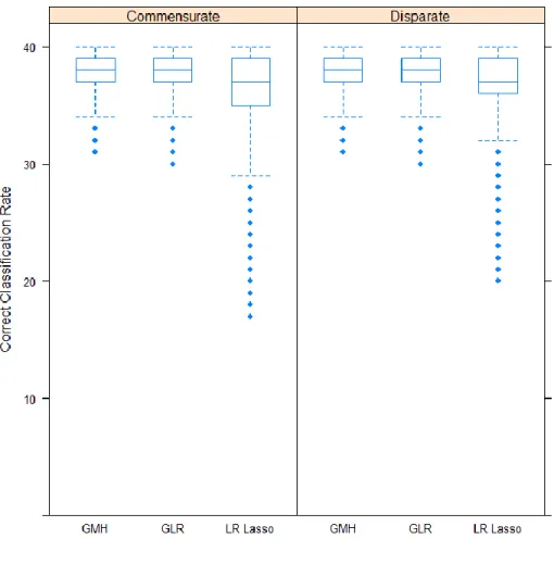
Page Figure 1. Contingency Table for Any Given Score Level, m. ... 19 Figure 2. Correct Classification Rates (in Number of Items) across All
Replications For Conditions Parsed by Commensurate and Disparate Locations of Test Information Targets Relative to Simulee
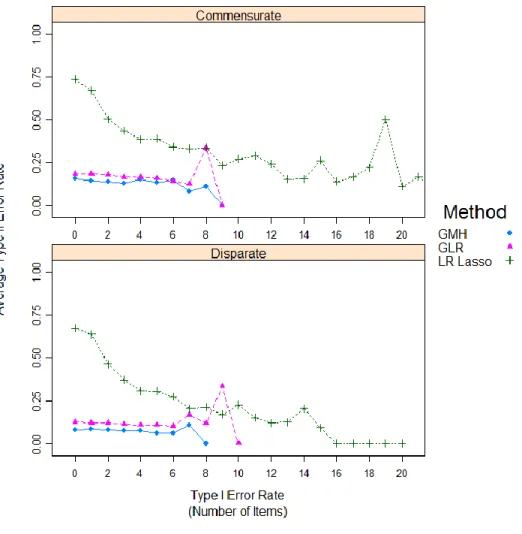
Populations. ... 77 Figure 3. Average Type II Error Rate (by Number of Items) for Various Levels of
Type I Error Rates Parsed by Commensurate and Disparate Locations
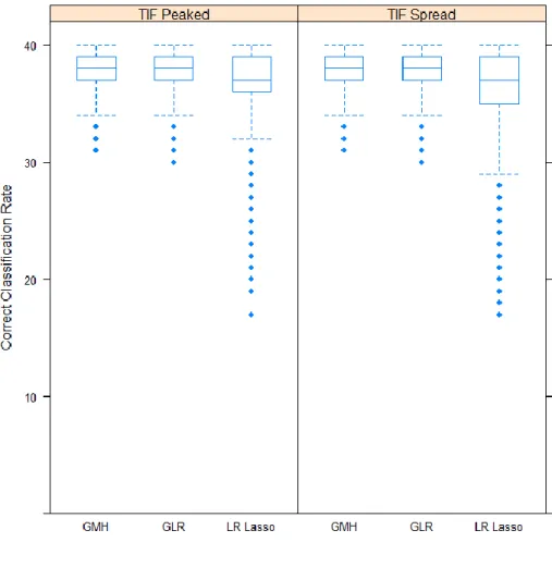
of Test Information Targets Relative to Simulee Populations. ... 78 Figure 4. Correct Classification Rates (in Number of Items) across All
Replications for Conditions Parsed by the Relative Spread of the Test
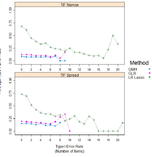
Information Function. ... 79 Figure 5. Average Type II Error Rate (by Number of Items) for Various Levels of
Type I Error Rates Parsed by the Relative Spread of the Test
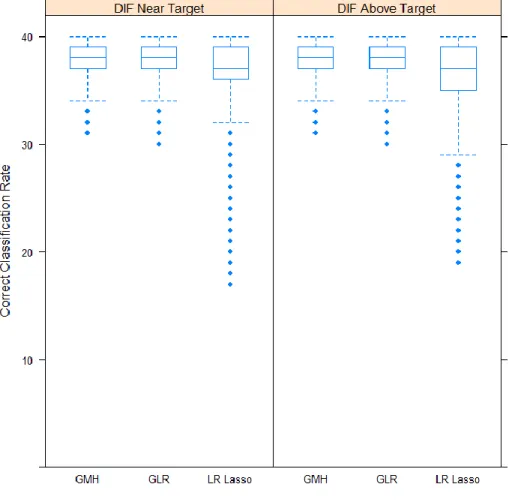
Information Function. ... 80 Figure 6. Correct Classification Rates (in Number of Items) across All
Replications for Conditions Parsed by Location of DIF Items
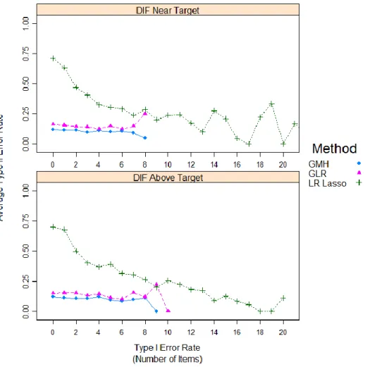
Relative to the Test Information Target. ... 81 Figure 7. Average Type II Error Rate (by Number of Items) for Various Levels of
Type I Error Rates Parsed by Location of DIF Items Relative to the
Test Information Target. ... 82 Figure 8. Correct Classification Rates (in Number of Items) across All
Replications for Conditions Parsed by Percentage of DIF Items. ... 83 Figure 9. Average Type II Error Rate (by Number of Items) for Various Levels of
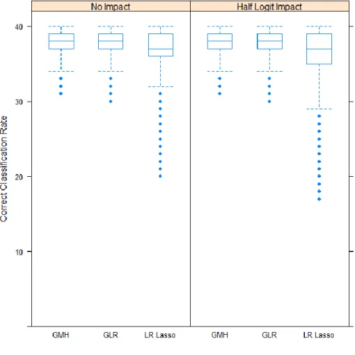
Type I Error Rates Parsed by Percentage of DIF Items. ... 84 Figure 10. Correct Classification Rates (in Number of Items) across All
Replications for Conditions Parsed by Presence of Impact. ... 85 Figure 11. Average Type II Error Rate (by Number of Items) for Various Levels
of Type I Error Rates Parsed by Presence of Impact. ... 86 Figure 12. Correct Classification Rates (in Number of Items) across All
x
Figure 13. Average Type II Error Rate (by Number of Items) for Various
Levels of Type I Error Rates Parsed by Sample Size Balance. ... 88 Figure 14. Correspondence of the Generating Ability Distributions and the
TIFs by Test Type. ... 90 Figure 15. Correspondence of the Generating Ability Distributions and the
TIFs by Location of DIF Items. ... 92 Figure 16. Correspondence of the Generating Ability Distributions and the
TIFs by Presence of Impact. ... 94 Figure 17. Magnitude of Penalty Parameters by Classification Type for
Scenario Three. ... 98 Figure 18. Magnitude of Penalty Parameters by Classification Type for
Scenario Four. ... 100 Figure 19. Magnitude of Penalty Parameters by Classification Type for
1 CHAPTER I INTRODUCTION
The overall purpose of this dissertation is to compare various observed score approaches in detecting differential item functioning among multiple examinee groups simultaneously. Specifically, this study contributes to the literature base by investigating a lasso-constraint observed score method in the context of multiple groups as well as features of test design related to test information targets. Given that a lasso-constraint method has not been extended for multiple groups using observed scores, comparisons are made with other observed score techniques while using item response theory to generate data (thus avoiding model-data congruity complications in the study design). To support the overall purpose, the scope of the current chapter includes background
information for differential item functioning, a detailed purpose and rationale, research questions, and definitions and notation of key terms used throughout the study.
Background of the Problem
Item-level bias in which the probability of a correct response among equally able persons differs in subgroups is known as differential item functioning (DIF; Tutz & Schauberger, 2015). DIF can also be defined as a violation of item-level invariance across subpopulations (Kamata & Vaughn, 2004). The Standards for Educational and Psychological Testing (hereafter referred to as the Standards; AERA, APA, & NCME, 2014) provides a formal definition of DIF:
2
Differential item functioning occurs when different groups of test takers with similar overall ability, or similar status on an appropriate criterion, have, on average, systematically different responses to a particular item (p.16).
It is important to clarify the difference between DIF and impact. Plainly stated, a group difference in ability or performance is not DIF. Impact refers to such differences in the overall distributions of the ability or performance of intact groups, and thus is a group-level measure (Dorans & Holland, 1993). DIF, on the other hand, is an item-level phenomenon. DIF is examined by first matching examinees in different groups on a criterion variable, typically ability or performance level. Because of this matching, DIF is unexpected as the groups have been made comparable with respect to the measured construct.
To distinguish between groups (usually demographic groupings), terms are used to describe relative advantage or disadvantage with respect to responding correctly on an item. The reference group is the group which may potentially have an advantage in answering the item correctly, while the focal group is the group of concern because they may potentially have a disadvantage in answering the item correctly. As an example within the context of testing in the United States, and in the case of the usual DIF methods that assume two groups, the reference group tends to be Caucasian American examinees while the focal group would be a combination of students from other racial groups. As another example, males may be considered the reference group and females as the focal group.
As it pertains to this study, when DIF is examined across more than two groups simultaneously there is one reference group and multiple focal groups. Given the
3
example of race described previously, the multiple groups of races would not be
combined into one focal group, but each group would remain intact for the analysis and each be treated as a unique focal group. Often, all focal groups are combined into a single focal group to alleviate issues related to balance between groups (i.e., statistical power) and pairwise comparisons (i.e., increased type I family error rates). When multiple focal groups are combined, there is an underpinning assumption that the groups have roughly the same ability distributions and potentially the same level of disadvantage on a given item. However, when the groups are not truly comparable, multiple group methods which allow the groups to remain separated are warranted.
Another example can be found whenever exams are administered in multiple languages (Angoff & Sharon, 1974; Ellis & Kimmel, 1992). Instead of designating English speaking examinees as the reference group and examinees with foreign language proficiency as a single focal group, each group of examinees speaking the same non-English language would be permitted to exist as an independent focal group. Still yet, additional examples could include large classrooms within a school, schools within a country, and longitudinal differences for an admissions test (Magis, Tuerlinckx, & De Boeck, 2015).
While the intention of this study does not specifically address the causes of DIF, it is important to understand some theoretical causes to underscore the importance of
testing for DIF. As an earlier reference, Jenson (1980) posited the cultural difference hypothesis, which described that people from different cultural backgrounds could have differing levels of familiarity with test content. In a similar manner, Meredith and Millsap
4
(1992) made the argument that manifest variables are not sufficient measures for
capturing the latent variables which actually cause DIF. To expand this idea, the manifest variables are correlated with the latent variables. For example, there is not an inherent physiological or psychological difference in intelligence between males and females which causes DIF; rather, there is likely a sociological/cultural phenomenon which reflects gender-normed behaviors and knowledge. Such phenomena are appropriately modeled as latent traits. However, latent variable procedures of DIF detection could suffer from model-data fit and estimation issues.
On the other hand, issues of DIF are not always cultural in nature. Examinees may simply use different metacognitive skills in responding to items (Tatsuoka, Linn,
Tatsuoka, & Yamamoto, 1988). Affective domains may also influence DIF, with such an example being females perhaps having an advantage with content involving social relationships (Stricker, 1981). Additional research supports this notion in finding that familiarity, interest, and emotional reactions may serve to be factors which impact item responses (Stricker & Emmerich, 1999). In the context of cross-lingual exams, Benítez and Padilla (2014) used cognitive interviews following quantitative DIF analyses to uncover that DIF may be caused by specific jargon which has different interpretations across languages.
DIF is influenced by and related to other phenomena. Once a DIF item has been flagged, it is important to explore what potentially is causing the item to be biased. Differential distractor functioning (or differential alternative functioning), differential speededness, and differential omission are analyses which can be used to better
5
understand why subgroups of examinees have differential performance (Dorans & Holland, 1993). As an example, Ben-Shakur and Sinai (1991) explored how differential guessing tendencies between males and females were influenced by formula scoring as opposed to number correct scores. Formula scoring was found to provide an advantage to males in both samples they examined (i.e., ninth graders and applicants to Israeli
universities).
Among some of the more empirical DIF studies are those which attempt to experimentally cause DIF. There are multiple strengths with these studies. First, they contain typical features of real data that simulation studies do not fully capture. Second, they avoid the model-data congruity issue which faces many simulation studies. Third, different causes of DIF, as well as various categorizations of subpopulations of
examinees, can be explored across multiple detection methods. However, there are no guarantees that an item intended to show DIF will do so. For example, a study by Scheuneman (1987) evaluated 16 hypotheses related to experimental (non-scored) test items which were manipulated to cause DIF on the Graduate Record Examination (GRE), and found that just 10 of the hypotheses supported DIF. The manipulations of item features were related to item format, vocabulary in antonyms, wording of the item stem, inference, test wiseness, key placement, and abstraction. Not all manipulations were detected as significant DIF.
Other studies have used experimental manipulation to induce DIF. A 50-item vocabulary test was constructed by Subkoviak, Mack, Ironson, and Craig (1984) which contained 10 items that favored black students over white students. Their findings
6
supported using the area between item characteristic curves (ICCs) corresponding with a unidimensional three-parameter logistic model (U3PL) to detect DIF, when compared with the transformed item difficulty index (Angoff & Ford, 1973; Angoff, 1982) and two chi-squared approaches (Scheuneman, 1979; Camilli, 1979). Kim and Cohen (1991) later reanalyzed the same data to elaborate on IRT-based area measures for detecting DIF. Other researchers have experimentally manipulated features of language to construct DIF items, and found that using an iterative logit method was appropriate for detecting DIF when it was supposed to exist (Kok, Mellenbergh, & Van der Flier, 1985). Still yet, others altered item order within content clusters between males and females, and found significant differences in calibrated IRT difficulties (Plake, Patience, & Whitney, 1988).
To combat the issues surrounding biased test items, the Standards (AERA, APA, & NCME, 2014) express the need for analyzing and reporting on issues surrounding item bias and, more specifically, DIF. In fact, chapter three in Part I of the Standards is
devoted specifically to issues pertinent to fairness in testing. As it relates directly to DIF, suggestions surround the need for preventing construct irrelevant variance at all steps of the testing process (3.0), including minimizing all sources of construct-irrelevant variance which could stem from linguistic, communicative, cognitive, cultural, physical, or other characteristics (3.2), as well as including all subgroups when pilot testing items to screen for bias (3.3). The Standards also describe the need for documenting procedures used in evaluating item quality, including screening for DIF among major examinee groups (4.10). Although, relatively few suggestions are provided in how to obtain these goals. In consideration, psychometricians are free to use their professional judgement as to what
7
methods are appropriate to use in a given scenario. Unfortunately, not all methodologies are comparable in performance, even when they are designed for similar situations. Therefore, it is crucial to understand how error can be introduced through choice of methodology alone.
Assuming that error associated with all those aforementioned portions has been successfully mitigated, there are errors potentially introduced by choice of methodology (which is one concern of this study). It is entirely possible that using a particular
statistical method to detect DIF may not work properly in certain scenarios. For example, some methods (such as logistic regression; LR) are known to contribute to increased type I errors (i.e., false positives) whenever overall group differences exist in the midst of guessing behavior by examinees (DeMars, 2010). Of particular concern is the level of type II error (i.e., false negatives), which occurs when items that truly exhibit DIF are not detected. Practically speaking, type I errors could potentially lead to good items being removed from exam scoring, while type II errors could potentially allow biased items to be included in determining exam scores.
An item which is flagged according to a statistical criterion does not necessarily mean that the item is biased against subgroups, nor does an item which is deemed appropriate guarantee that the item is not biased. Detecting DIF items is further complicated by data requirements and assumptions with more complex DIF detection techniques. Selecting a method which is too complex may accidentally result in modeling noise along with signal found in data because the model contains more parameters than necessary for describing the data. As such, it is possible that placing statistical constraints
8
(e.g., a lasso constraint) on existing methods may improve performance in these instances.
Determining which items possess DIF in a given test can vary depending on the DIF detection method chosen, given that each method has different assumptions. While these differences are practically non-existent under ideal testing conditions (e.g., large numbers of examinees, excellent model-data fit, and unidimensionality), data which are not ideal will exacerbate differences between the methods. Unfortunately, matters are further complicated by the possibility of multiple types of DIF.
Distinguishing between multiple types of DIF is important because DIF detection methods may be better suited for particular types of DIF. As such, different causes of DIF often result in different types of DIF. When considering item response functions, DIF can be viewed as uniform or non-uniform. Uniform DIF occurs whenever the same group is favored at any level of ability or performance. Stated differently, there is no meaningful interaction between group membership and ability level. This type of DIF is typically associated with a between-group difference in the difficulty of a given item. Uniform DIF frequently occurs if the DIF occurs in the correct response option, though it can also appear in the question stem, distractors, or supporting materials when answering an item.
On the other hand, non-uniform DIF generally refers to when the relative advantage at any given level of ability or performance changes with respect to the other group(s). In other words, there is a meaningful interaction between group membership and ability. Non-uniform DIF can be observed as uniform crossing DIF or non-uniform crossing DIF. In the former case, typically both the difficulty and discrimination
9
of an item change across groups in such a way that the item response functions do not intersect at any point along the ability continuum. In the latter case, the primary between-group difference is the item discrimination, which causes the item response function to intersect at or near the difficulty of the item. This type of DIF is rarer, and is an
interesting find because the relative advantage reverses depending upon what point of the ability continuum is observed. For example, focal group examinees with higher ability may be disadvantaged on the item while examinees with lower ability are advantaged when compared with the reference group.
While multidimensional approaches can be used to account for secondary traits (e.g., SEM and MIRT), such traits which cause DIF are undesirable and cannot justifiably be supported as appropriately entering the item writing process as long as a single score is reported for interpretation and use. Nevertheless, one possibility could be to model a secondary dimension, and base the scoring using only parameters of the primary dimension. However, these modeling procedures can be complex and may not lead to stable estimates. Observed score approaches offer a parsimonious way of detecting DIF, and are used by major testing organizations (e.g., ETS, ACT) even in the present time.
The peculiar nature of detecting DIF is that many statistical tests for doing so analyze one item at a time, making an inherent assumption that there is not contamination in the total score introduced by other items. That is, an assumption is made that all other items except the one under examination are non-DIF items. However, this assumption is not necessarily the case, and is a very strict requirement to meet. Most DIF methods are performed at the item level, but approaches which fit a global model and can estimate
10
item-level parameters is a potential strategy that is less restrictive in the assumptions made on items.
As a way to control for ability level, many DIF models use the observed total score (i.e., a proxy for ability) as a matching criterion to match examinees between groups. This matching helps to lessen the chances that differences observed at the item-level are influenced by differences in group ability (i.e., impact). However, if there are one or more DIF items on an exam, the matching criterion will be contaminated by construct-irrelevant variance. One strategy to potentially improve the matching criterion is item purification (Candell & Drasgow, 1988; Holland & Thayer, 1988; Lautenschlager & Park, 1988; Clauser, Mazor, & Hambleton, 1993; Fidalgo, Mellenbergh, & Muñiz, 2000; Wang & Yeh, 2003; Wang & Su, 2004; as cited in Magis, Beland, Tuerlinckx, & De Boeck, 2010). Item purification is an iterative procedure which removes DIF items from the calculation of a total score or estimation of ability. A DIF method which is calculated for each item individually is first used. Any items with DIF are removed, and the calculations are performed again using the remaining items which were determined to be free of DIF. These steps are continued until none of the remaining items are flagged as having DIF, and the remaining items are used to determine the total score or ability estimate for matching. While purification minimizes issues related to DIF influencing the matching criterion, it introduces an additional confound if many items are removed because there are less data being used to determine the matching variable.
The matching variable, even with improvements or estimation with a latent trait model, is not a perfect representation of ability. Absolute truth cannot be known with a
11
latent trait, nor can it be known in regards to how subgroups of examinees will interact with items. Consequently, it benefits greatly to speculate situations where the truth is assumed be to known, and deviation from truth can be quantitatively measured. Simulation studies accomplish this feat, which allow for absolute manipulation of a constructed reality (Baudrillard, 1994). That is, a study can be conducted which
purposefully creates simulated data that contain DIF items, and various methods can be directly compared in how well they correctly identify DIF, as well as fail to recognize it.
Purpose and Rationale
Demographic information is often collected for variables which have more than two groups (e.g., race/ethnicity and language), and being able to explore DIF with these variables provides the exigency of this inquiry. Multiple researchers have asserted that a limitation of most existing DIF methods is that only two groups can be tested (Penfield, 2001; Tutz & Schauberger, 2015; Oshima, Wright, & White, 2015). The purpose of this proposed study is to compare and contrast more traditional multiple group observed score (i.e., non-IRT) DIF detection methods (e.g., generalized Mantel-Haenszel χ2 and
generalized logistic regression) with the more recently developed logistic regression lasso DIF technique (LR lasso DIF; Magis, Tuerlinckx, & De Boeck, 2015). In fact, this
purpose was suggested by the authors:
The method can easily be extended to more than two groups of respondents. It is straightforward to extend the definition of the DIF to any number of groups and to perform lasso penalization onto all DIF parameters for all groups simultaneously. One can then determine on the basis of the lasso approach which items function differently between which groups of respondents. The LR method has been
12
2011; Magis & De Boeck, 2011), so that it can be used as a basis of comparison (p. 131).
Additionally, this study adds to the literature base through exploring how features of test design, specifically those surrounding information targets, may affect the extent to which DIF items can be correctly identified. A simulation study will be used to
demonstrate and summarize scenarios which distinguish between the performances of the methods in detecting true DIF items. The proposed study aims to inform practitioners and researchers of situations where they may find the results useful in judging the merit of adopting the newer lasso method for detecting DIF within multiple groups as opposed to using the pre-existing methods. While several studies have explored detecting DIF in multiple groups, there are no studies to date which explore to use of lasso constraints while detecting DIF among multiple groups using observed score approaches. It is worth mentioning, however, that a recently developed DIF procedure for the Rasch model by Tutz & Schauberger (2015) examined its performance when there are multiple simulated groups. Applying the lasso constraint in the context of multiple groups has not been done for an observed score approach, and this study aims to fill the gap in the literature.
However, observed score approaches have several limitations (Spray, 1989). First, an observed test score is not a perfect representation of an examinee’s latent ability, given that the measured scale is not perfectly reliable and is influenced by various sources of measurement error. Second, the observed scores reflect sampling errors. There is no guarantee that the samples for each subgroup are reflective of their respective populations, especially when sample sizes of particular subgroups decreases. Third,
13
because observed scores are summed across individual item scores, items with DIF directly influence the matching variable in an observed score DIF method. Thus, creating a study which manipulates variables related to these limitations advances the
understanding of DIF detection in the presence of multiple groups. Research Questions and Study Variables
This study was guided by two main research questions, each of which is composed of several subquestions. The aim of the first research question was to determine the comparability of the observed score DIF methods with respect to classification accuracy of DIF items. The evaluation of the DIF methods based upon absolute criterion are examined in subquestions 1a through 1d, because the ultimate goal of DIF methods is to correctly detect items which are biased against subgroups. These subquestions consider correct classification, type I error, type II error (specified in terms of hit rates), and consistency with truth. Subquestion 1e concerns relative comparisons among the methods by determining the extent to which they classify DIF items in a similar manner.
The second research question was posited to determine how the methods are directly influenced by changes in types of independent variables which are commonly considered in DIF studies. These subquestions are directly related to the simulation conditions that are manipulated in this study. Specifically, visual inspection of conditional plots can answer what proportion of error can be directly attributed to characteristics at the test-level (e.g., the location of the information target relative to the examinee population and the shape of the test information function; subquestions 2a, 2b,
14
respectively), the item-level (e.g., the location of DIF items relative to the information target and the percentage of DIF items; subquestions 2c, 2d, respectively), and of simulees (e.g., the amount of impact and sample size; subquestions 2e, 2f, respectively). Specifying the research questions in this manner allowed for the interaction between simulation conditions to be examined, as opposed to examining each condition only in isolation. The research questions are explicitly stated as the following:
1. How does the penalized LR DIF detection method (i.e., LR lasso) compare to more traditional non-IRT multiple-group methods (i.e., generalized Mantel-Haenszel χ2 and generalized logistic regression) as it relates to:
a. correct classification rate of DIF items?
b. type I error rate in the classification of DIF items?
c. hit rates (defined as one minus the type II error rate) in the classification of DIF items?
d. phi correlations of true and detected DIF items? e. agreement statistics among methods?
2. When detecting items that truly exhibit DIF, to what degree is classification error for each analysis model influenced by changes in:
a. the location of the information target relative to the examinee population? b. the shape of the information function?
c. the location of DIF items relative to the information target? d. the percentage of DIF items?
15 e. the amount of impact?
f. sample size?
Definition of Key Terms and Notation
A list of select terminology and abbreviations is provided in Table 1. The hope is that this table serves as a quick and accessible reference for readers as they encounter unfamiliar abbreviations and to clarify terminology that may be ambiguous due to multiple existing definitions. More detailed descriptions are provided throughout the text of this document where relevant.
Study Organization
A total of five chapters are used to describe this study in-depth. The current chapter was an introduction to DIF and described the importance of this study to the measurement field. In order to frame the study purpose and research questions, a review of relevant DIF literature is summarized in Chapter Two. Chapter Three is used to specify the simulation study design along with the methodologies that will be used to evaluate the results for each research question and subquestion. Chapter Four contains a presentation of the results, accompanied by summary tables and figures. Finally, Chapter Five comprises a discussion of the results, with consideration given to comparisons alongside the DIF literature more generally.
16
Table 1. List of Selected Terms and Notation Along with Brief Definitions
Term Description
ai item discrimination
bi item difficulty
ci item lower asymptote for probability of correct response
χ2 chi-squared
D scaling constant (i.e., 1.000 or 1.702) used in logistic IRT models DIF differential item functioning
ETS Educational Testing Service ICC item characteristic curve IRF item response function IRT item response theory
GMH generalized Mantel-Haenszel GLM generalized linear model
GLR generalized Logistic Regression GRE Graduate Record Examination
k number of items LR logistic regression MH Mantel-Haenszel N number of examinees/simulees Q1 first quartile Q3 third quartile R right
TCC test characteristic curve TIF test information function
θn examinee/simulee ability level
U2PL unidimensional two-parameter logistic model U3PL unidimensional three-parameter logistic model
W wrong
X total score obtained for the entirety of Form X xi item score obtained for item i on Form X
17 CHAPTER II LITERATURE REVIEW
The current chapter is organized by first providing a synopsis of observed score approaches to detecting DIF, with descriptions flowing from simpler to more complex models for each of the three analysis models used in this study. Subsequent sections are devoted to providing background research related to conditions which are manipulated later in the simulation study that have been considered in previous studies. Finally, an overview of item response theory (IRT) is provided to inform later discussions
surrounding the data generation model. While the emphasis of this study is observed score approaches, some literature from IRT approaches may appear because LR and IRT share similarities under the generalized linear model (GLM).
Overview of Observed Score Multiple Groups DIF Methods
The following section provides a brief overview of the statistical techniques using observed scores to detect DIF items. Readers interested in more detailed coverage are referred to the foundational articles for each of the methods (as provided in each section). The models discussed hereafter are used as the analysis models later in this study.
Mantel-Haenszel and Generalized MH
The development of DIF indices historically has included non-parametric approaches. In educational measurement, two similar approaches based upon χ2 (chi-squared) were suggested in the late 1970s (Subkoviak, Mack, Ironson, & Craig, 1984). Scheuneman (1979) proposed a procedure similar to χ2 which used only correct item
18
responses to determine DIF. By conditioning on total score as a proxy for ability, the procedure calculated the probability of a correct response for each possible observed score category. Items with unequal probabilities across score categories were identified as DIF items. In the same year, Camilli (1979) described a χ2 statistic which used both correct and incorrect responses to reach a very similar statistical test. The strength of these conditioning procedures is that they do not make assumptions regarding the score distributions for each group. However, this type of non-parametric conditioning
procedure was actually described decades before.
Mantel and Haenszel (1959), outside of the context of educational statistics and psychometrics, introduced a χ2 procedure which allowed for a comparison of matched groups. The resulting statistical test is traditionally referred to as Mantel-Haenszel χ2 (MH). It was later adapted by Holland and Thayer (1988; Holland, 1985) for detecting DIF as a hypothesis test on the constant odds ratio of getting an item correct for two groups across all ability levels.
An item is considered to possess DIF when the MH test statistic exceeds a critical value that is established a priori. The calculation of MH is based upon a three-way contingency table (see Figure 1), with dimensions for the matching criterion (typically integer values spanning the range of observed values of the total score), frequencies of correct and incorrect item responses (or score categories in a polytomous case when using a generalized model), and categories (typically group membership for two groups, or more than two groups in a generalized model). The resulting MH statistic follows an asymptotic χ2 distribution with one degree of freedom (see Equation 1). The MH formula
19
differs from the usual χ2 formula because the denominator term is not the expectation, and the summation is over the matching criterion as opposed to all observations within a single contingency table. This difference is because MH conceptually (and not
algebraically) is summing across individual χ2 tests conditional on the matching criterion. MH also incorporates Yate’s correction for continuity by subtracting 0.5 from the
absolute difference in the numerator. To calculate Equation 1, the expectation (see Equation 2) and the variance (see Equation 3) terms are needed.
Figure 1. Contingency Table for Any Given Score Level, m. This Figure Has Been Adapted From the One Provided by Dorans & Holland (1993).
The null hypothesis (see Equation 4) states that there is no conditional association (i.e., across all permissible total scores, or bins/strata of score levels in scenarios with smaller sample sizes) between group membership and responding to an item correctly. The alternative hypothesis states that there is a conditional association between group membership and item response. Furthermore, the conditional association is a consistent, unidirectional difference (i.e., uniform DIF).
m rm m rm m rm R Var R E R ) ( 5 . ) ( 2 2 (1)20 N R N R E tm tm rm rm) ( (2) ) 1 ( ) ( 2 N N W N R N R Var tm tm tm fm tm rm rm (3) 1 : 0 W R W R H fm fm rm rm (4)
An effect size measure of MH (αMH; see Equation 5) was provided by Mantel and Haenszel (1959). In view of the fact that the interpretation of odds ratios are bounded between zero and positive infinity, the log-odds of αMH (see Equation 6) are typically calculated so that the values are theoretically bounded between negative infinity and positive infinity, and are asymptotically normally distributed (Agresti, 2002). Sometimes, this calculation is linearly translated to the delta metric to ease interpretation of the log-odds. ETS, as well as some other companies, use a transformation of the common-odds ratio for interpretation, a statistic known as MH D-DIF (see Equation 7; Holland & Thayer, 1988; Dorans & Holland, 1993).
N W R N W R tm m fm rm tm m rm fm MH ) * ( ) * (
(5) ) ln( MH MH (6) MH DIF D MH 2.35* (7)21
Significantly positive values of MH D-DIF suggest that an item is biased against the focal group, while negative values of MH D-DIF suggest that the bias is against the reference group. A three-category classification system was developed to describe the magnitude of DIF detected in an item (Dorans & Holland, 1993). The three levels are “A” (negligible DIF), “B” (intermediate DIF), and “C” (large DIF). The absolute values of MH D-DIF, or the MH-LOR, are used along with significance testing to determine the level of DIF that an item exhibits. An item is designated as Level A if |MH D-DIF| is less than 1.0 delta unit (or |MH-LOR| < .426) or |MH D-DIF| is not significantly different from 0. An item is designated as Level C when both |MH D-DIF| is greater than 1.5 delta units (or |MH LOR| ≥ 0.638) and is significantly greater than 1.0. By default, any items which do not belong to Levels A or C are classified into Level B.
The MH approach to detecting DIF makes a few assumptions. First, it inherently assumes unidimensionality of the scale score, given that a single total score is used to perform the matching for the hypothesis test. Second, the direction of bias between the two groups is assumed to be unidirectional across all levels of the matching variable, which means that MH is truly appropriate for detecting uniform DIF only. Third, a hypergeometric assumption is made with regards to the marginal totals. In calculating the expected values for the χ2 statistic, the marginal totals are assumed to be fixed at a given total score (or stratum). While the χ2 statistic is non-parametric, the resulting value is sample-dependent. Fourth, it is assumed that the two groups in the test are independent of each other. However, it is often the case that there are shared characteristics or
22
dependencies between the two groups (e.g., males and females may be similar with regards to school, community, culture, and socio-economic status).
In the context of multiple groups, it is not appropriate to conduct a test of DIF for each focal group separately. As Penfield (2001) notes, there are three limitations to doing so: (1) inflated type I error rates; (2) decreased statistical power to detect DIF; and (3) increased run-time and computing resources. Alternatively, it is better to test for DIF among all groups simultaneously. The generalized Mantel-Hanszel procedure (GMH; Mantel & Haenszel, 1959; Somes, 1986) can be used to detect uniform DIF among multiple groups. In addition to better controlling for issues with statistical power, this technique also controls the type I error rate without requiring post hoc adjustments to familywise-error rates such as the Bonferonni correction or adjustments to the false discovery rate such as the Benjamini–Hochberg procedure (Kim & Oshima, 2013). Additionally, it also makes no assumptions concerning the cause of the item responses (unlike IRT-based approaches).
GMH is essentially a measure of average partial association in a three-way contingency table. It differs from MH in that it potentially allows for more than two groups and/or polytomous item scores. Furthermore, it is potentially advantageous for use on polytomous data because it does not assume that the data are ordinal, and looks across the distribution of item scores without assuming a particular distributional form. The calculation for GMH χ2 is given by Equation 8. The GMH χ2 statistic is chi-squared distributed, with the degrees of freedom under the null hypothesis being equal to one less than the number of demographic groups (assuming dichotomous data, which simplifies
23
the second degree of freedom in the set). Like MH, the null hypothesis under GMH is no conditional association between group membership and response category.
The formula contains bolded letters to indicate vectors of values. The vectors Ak (see Equation 9) and E(Ak) (see Equation 10) have a length one less than the number of groups (i.e., G-1), and V(Ak) is a covariance matrix of the same rank (see Equation 11). The vector Ak is analogous to the Rrm term from MH, and it represents the pivotal cells for each level of the matching variable. The expectation of this vector is given by
Equation 10, and its variance in Equation 11. The plus sign that is included as a subscript indicates summation over that dimension. A general form of GMH also was given by Landis, Heyman, and Koch (1978) which allows it to more directly simplify to the MH procedure (as cited by Zwick, Donoghue, & Grima, 1993).
( ) ' ( ) 1 ( ) 2 A E A A Var A E A GMH k k k k k (8) 𝑨𝒌= (𝑛11𝑘, 𝑛12𝑘, ⋯ , 𝑛1(𝐺−1)𝑘) (9) 𝑬(𝑨𝒌) = 𝑛1+𝑘𝒏𝑘′ 𝑛++𝑘 (10) 𝑽(𝑨𝒌) = 𝑛1+𝑘𝑛0+𝑘(𝑛++𝑘𝑑𝑖𝑎𝑔(𝒏𝑘)−𝒏𝑘𝒏𝑘′ 𝑛++𝑘2 (𝑛++𝑘−1) ) (11)Additional advantages of using GMH include increased power under balanced designs, as well as not collapsing focal groups in a manner such that truly differential performance is subsequently undetected. While not considered in this study, GMH has a stronger literature base with applying the procedure to polytomous data, as opposed to
24
multiple groups (Welch & Hoover, 1993; Zwick, Donoghue, & Grima, 1993; Zwick & Thayer, 1996; Chang, Mazzeo, & Roussos, 1996; Zwick, Thayer, & Mazzeo, 1997; Ankenmann, Witt, & Dunbar, 1999; Camilli & Congdon, 1999; Penfield, 2001; Penfield & Algina, 2003; Meyer, Huyah, & Seaman, 2004; Wang & Su, 2004; Su & Wang, 2005; Kristjansson, Aylesworth, McDowell, & Zumbo, 2005). The limitations of GMH are that it cannot discern between uniform and nonuniform DIF (Kristjansson, Aylesworth, McDowell, & Zumbo, 2005), the power of the procedure is decreased by smaller sample sizes and impact (Welch & Hoover, 1993, as cited in Penfield & Lam, 2000), and type I errors may possibly be inflated when impact is present (Welch & Hoover, 1993). Logistic Regression and Generalized LR
As described by Agresti (2002), the generalized linear model can be described as composed of three components: the random component (i.e., the dependent variable and its probability distribution), the systematic component (i.e., the independent variables), and the link function (i.e., the relationship between the independent variables and the dependent variable). When predicting a dichotomous outcome, the GLM can be
expressed as a logistic regression. More specifically, a logistic regression is expressed by having mixed effects independent variables (i.e., categorical and/or continuous
predictors), a binomial dependent variable, and a logit link. Whenever the GLM is constrained using the logit link it is often referred to as a logit model.
Unlike linear regression, LR makes no assumptions regarding normality, linearity, homogeneity, and normally distributed error terms (Howell, 2010). However, the
25
method used makes additional assumptions in addition to those of the model itself. The model parameters of LR cannot be estimated using least squares methods due to the logit link, so maximum likelihood estimation (MLE) methods are typically used to perform the model estimation. Additionally, estimates are solved under MLE using iterations because no closed form solution exists. MLE assumes that data are independently drawn from a multivariate normal distribution (Myung, 2003).
The premise behind LR as a DIF detection method is to predict item responses when using total scores and group membership as predictors. In short, an item is determined to be DIF based upon testing regression coefficients for statistical significance. The first substantial mention of an LR-like approach as a possible DIF detection method (in a non-IRT context) was made in the early-to-mid 1980s (Van der Flier, 1980; Mellenbergh, 1982; Van der Flier, Mellenbergh, Ader, & Wijn, 1984). An iterative logit model was used to correct for the influence that DIF items have on the total score, which is typically a limitation of observed score methods (others have used
purification techniques to accomplish the same feat). This method built upon the contingency table approaches by using loglinear models to analyze the data, which is comparable to using the odds ratio estimator in the MH technique. Much like the later LR method for DIF detection (Swaminathan & Rogers, 1990), this method modeled the item difficulty as the intercept, and included parameters for the observed score category and group membership, in addition to an interaction effect of score category with group membership. However, it differed from the later LR method because it treated the observed scores as discrete unordered categories.
26
More in line with the usual LR framework for dichotomous data with two groups, an LR framework was being studied prior to the more formal conception of the LR method (Spray & Carlson, 1986; Bennett, Rock, & Kaplan, 1987). Swaminathan and Rogers (1990) were the first to provide a detailed model which improved upon IRT methods by reducing issues related to sample size and model-data fit, and improved upon the previous logit models by better accounting for the continuous nature of the ability scale.
Swaminathan and Rogers (1990) further provided a conceptual relationship between MH and LR which involves constraining the LR. Two assumptions must be made. First, the ability variable must be discrete (e.g., observed total scores). Second, there must be no interaction term between the ability variable and group membership, which excludes testing for non-uniform DIF. While this relationship is not exact (given that MH is non-parametric and LR is parametric, and both are based on different assumptions), the hypothesis for uniform DIF is being tested in both.
However, Swaminathan and Rogers (1990) demonstrated that LR was more effective than MH in detecting non-uniform crossing DIF in their foundational paper, particularly across varying test lengths and sample sizes. Using the notation of Magis, Tuerlinckx, and De Boeck (2015) to keep consistency with their model described later, the LR model specified by Swaminathan and Rogers is given by Equation 12.
G S
Y
27
Using a logit link, the model specifies the probability of a correct response (Y=1) to a single dichotomously scored item, j, for examinee i belonging to group g. The intercept term, α0j, is related to the difficulty of the item. The first logistic regression coefficient, α1j, gives the change in log-odd units of the item-level scores for a single unit increase in the total test score, Si, of examinee i. The second logistic regression
coefficient, α2j, describes the change in log-odd units of the item-level scores for a change in group membership from the reference group (0) to the focal group (1). This latter coefficient is of primary importance, because there should be no discernable difference with respect to item performance between the reference and focal groups.
While there are multiple approaches to testing the null hypotheses, primarily two methods have been used in prior studies: the Wald test (Wald, 1939) and the likelihood ratio test. Both approaches are similar in that they can be conceived as being nested model comparisons, and they both share the same asymptotic chi-squared distribution. The Wald test is a significance test of a vector of parameters used to see if each
parameter is significantly different from zero. Non-significant parameters can
subsequently be omitted from the model. The Wald test was used by Swaminathan and Rogers (1990), which is a good reference for interested readers. As an alternative, the likelihood ratio test, not to be confused with the IRT-based DIF detection technique having the same name (Thissen, Steinberg, & Wainer, 1988), compares null and alternative hypotheses within the nested model comparison. The formula for the likelihood ratio test is provided in Equation 13. In words, Wilks’ lambda (Λ; Wilks,
28
1938) is equal to double the opposite of the natural log ratio of the maximized likelihoods of the nested models, where L0 is the null model and L1 is the alternative model.
L L 1 0 ln * 2 (13)
Table 2 highlights the comparisons made with respect to the model parameters. The basic model is written in abbreviated form, S + G + S*G, to indicate the predictors for observed score (S), group membership (G), and the interaction term (S*G).
Table 2. Comparison of LR Model Parameters for the Three Null Hypotheses Tested in the Likelihood Ratio Test.
DIF Type Null Alternative Difference in
Nested Models
Uniform S + G S G
Non-Uniform S + G + S*G S + G S*G
Both S + G + S*G S G + S*G
Magis, Raîche, Béland, and Gérard (2011) were the first to build upon the LR technique to create a generalized model, namely the GLR method of DIF detection. As noted in their paper, Millsap and Everson (1993) suggested that LR could be expanded into the GLR. Moreover, Van den Noortgate and De Boeck (2005) presented a logistic mixed model capable of considering multiple groups, which was essentially a
reformulation of an IRT model. Although flexible, their model involved the estimation of ability, which is circumvented in the GLR because it is an observed score approach. And compared with the GMH, the GLR potentially allows for a more direct detection of non-uniform DIF through a significance test on its interaction term. However, if a test only
29
possesses one or more items with uniform DIF, including the interaction term in the model could potentially lessen the chance that uniform DIF is properly detected.
Equation 14 is the model equation for the GLR, where πig is the probability that respondent i from group g responds correctly to a dichotomous item. The reference group is g = 0, and non-zero values represent the focal groups. The common intercept and slope are given by α and β, respectively. The specific intercepts and slopes are given by αg and βg, where the specific coefficients for the reference group (i.e., α0 and β0) are constrained to be equal to zero. This constraint allows the interpretation of the focal group
coefficients to be relative to the reference group. Three null hypotheses are included in the model. The null hypothesis for uniform DIF (see Equation 15) is characterized by uniform DIF being present if at least one intercept is significantly different from zero while having all slope parameters equal to zero. On the other hand, the null hypothesis for non-uniform DIF (see Equation 16) states that non-uniform DIF is characterized by at least one slope being significantly different from zero, irrespective of the value of the intercept parameters. Taken together, the null hypothesis for both types of DIF (see Equation 17) requires that all parameters be equal to zero across groups.
0 ) ( ) ( 0 ) ( g if g f logit S i S i g g i ig
(14) (UDIF) 0 ... | 0 ... : 1 1 0 F F H (15) (NUDIF) 0 ... : 1 0 F H (16)30 (DIF) 0 ... ... : 1 1 0 F F H (17)
Seeing as the GLR has three null hypotheses and explicitly tests for non-uniform DIF, it theoretically has a benefit over the GMH. However, a potential limitation of GLR is that increasing the number of groups potentially also increases the type I error rate. Furthermore, the use of maximum likelihood in GLR could potentially be a limitation whenever item scores are subject to variance restriction because of extreme difficulty values.
Logistic Regression Lasso Approach
In linear algebra, vector norms are used to regularize estimation of prediction models. Two common examples of vector norms are the L1-norm (i.e., lasso) and L2-norm (i.e., ridge regression), which serve as penalties in regularized estimation of a generalized linear model. Both are used to place constraints on model parameters. A major difference is that the lasso performs the shrinkage of parameters towards zero using absolute values, while ridge regression uses sum of squares to perform the
penalization. In doing so, the lasso translates coefficients by a constant factor, while ridge regression scales coefficients by a constant factor. The translation allows the former to successfully obtain values of zero, and permits variable selection through the remaining non-zero coefficients. Ridge regression, on the other hand, does not perform variable selection and is not appropriate for DIF analyses because it cannot discern between predictors at the item-level.
Recall that when the GLR is estimated, it performs the model parameter estimation through an item-by-item basis. The LR lasso DIF method provides a
31
theoretical improvement over the GLR by fitting a generalized linear model to an entire data set. The global nature of LR lasso allows for the relationships between items to be better captured. However, it does not escape the ipsative nature of DIF (i.e., the total score is a property of the test and not an external criterion). LR lasso places the lasso constraints on the variables for each item that describe differences in item performance given group membership. That is, not all items have a meaningful difference in group performance that should be explicitly modeled. Described within the context of LR lasso, logistic regression is a special case of the generalized linear model that can be estimated using lasso regularization. In fewer words, the LR lasso is a lasso penalized version of a generalized logistic regression. The lasso is performed using penalty terms (λ), which cause it to be a shrinkage estimator. Estimated coefficients for covariate terms (e.g., group membership) are multiplied by λ. Other LR terms (e.g., item difficulty and test score) are not influenced by λ.
The LR lasso model (see Equation 18) bears resemblance to the original LR DIF method by having coefficients for test score and group membership. However, the coefficient for test score, Si, is constrained to be the same for all items for two reasons.
First, it circumvents problems with model inconsistency because allowing items to be weighted differently is akin to a weighted sum, and defeats the purpose of using an observed score method where the total score is a sufficient estimate of ability. In this respect, the LR lasso model is more akin to the U1PL model than the U2PL model. Second, allowing different item weights potentially increases the type II error rate (DeMars, 2010, as cited in Magis, Tuerlinckx, & De Boeck, 2015).
32
G S
Y
Logit[Pr( ijg1)]0j1 i2j ig (18)
Given that MLE fits the entirety of the data, the penalized log likelihood (see Equation 19) must be maximized with respect to a vector of all parameters (see Equation 20) simultaneously. For model identifiability, a constraint is added so that α21 is equal to zero. Given the summation of α2j in the penalized log likelihood, the estimated difference across all groups is multiplied by the penalty parameter, λ. The product of those two terms is referred to as the penalty term.
J j j l 1 2 | | ) ( max arg ) ( τ τ ^ (19) ) , , , , , , (01 ... 0J 121 ... 2J τ (20)
The optimal λ value can be determined based upon two primary methods. The first is using relative fit statistics describing information criteria (not to be confused with information in IRT), such as Akaike information criterion (AIC; Akaike, 1974), AIC correction for finite samples (AICc; Hurvich & Tsai, 1989; Burnham & Anderson, 2002), Bayesian information criterion (BIC; Schwarz, 1978), Corrected AIC (CAIC; Bozdogan, 1987), Hannan–Quinn information criterion (HQIC; Hannan & Quinn, 1979), or
weighted information criterion (WIC; Magis, Tuerlinckx, & De Boeck, 2015). Another method is cross-validation (CV; Hastie et al., 2009). CV splits data into a number of subsets (k), and the prediction error is accumulated through k-1 iterations in which each subset is removed and the model is refit during each iteration. To provide a comparison,
33
CV is used to select a λ value which minimizes prediction error, while BIC is used to provide the most parsimonious/conservative solution.
The WIC is advocated by Magis, Tuerlinckx, and De Boeck (2015) because it provides an intermediate solution which differs from CV but also falls between the AIC (which is liberal) and the BIC (which is conservative) criteria. They reported that it outperformed the AIC, BIC, and CV criteria under most conditions for percentage of DIF items, DIF magnitude, and sample size and balance. WIC is a weighted average of AIC and BIC that allows the weighting for each to be influenced by characteristics of a given data set, such as sample size and number of items, because of how deviance terms and degrees of freedom are used in the calculation. Equation 21 provides the formula for WIC. The optimal penalty value is found by minimizing the WIC criterion conditional on ωi, where i refers to the weights on an interval inclusive of zero and one.
) ( * ) 1 ( ) ( * ) | ( AIC BIC WIC i i i (21)
Item Response Theory and Dichotomous Data Models
IRT models exist for both unidimensional and multidimensional data, though the former is explicated herein to provide necessary background and justification for the simulation conditions described later. In educational testing, IRT models describe the probability of a correct response for an examinee with a given ability (θn) to a particular
34
used to characterize how the probability of a correct response changes as ability-level changes.
The most widely used models have three or fewer parameters in describing the item properties. These three properties are difficulty (bi), discrimination (ai), and lower
asymptote (ci; also known as pseudo-guessing). Defined more specifically, item difficulty
is the location on the ability scale where the probability of a correct response equals .5 plus half of the lower-asymptote parameter, and is also the location on the θ scale where the inflection of the ICC occurs. Item discrimination is related to the slope of the item characteristic curve at the point of inflection, and is intended to model the extent to which an item can be used to distinguish between examinees of lower and higher abilities than the item difficulty. The lower asymptote sets a lower bound to the probability space, and is typically used to partially buffer for the impact of guessing in scored responses and improve model-data fit. It represents the probability of a correct response for an examinee with infinitely low ability.
The unidimensional three-parameter logistic model (U3PL) uses all three of the aforementioned item parameters along with θn to calculate the probability of a correct
response (see Equation 22). A scaling constant, D, of 1.702 has been used historically to allow the cumulative distribution function of the logit model to approximate that of a probit model. However, this practice has largely fallen out of favor, and the scaling constant usually equals one to retain the logit scale. Whenever ci is constrained to be
equal to zero across all items, the model reduces to the unidimensional two-parameter logistic model (U2PL). Additionally, both ai and ci can be constrained to one and zero,