The declining U.S. equity premium

(1)

Federal Reserve Bank of Minneapolis Quarterly Review

Vol. 24, No. 4, Fall 2000, pp. 3–19

The Declining U.S. Equity Premium

Ravi Jagannathan Ellen R. McGrattan Anna Scherbina

Chicago Mercantile Exchange Senior Economist Instructor

Distinguished Professor of Finance Research Department Department of Finance Kellogg Graduate School Federal Reserve Bank Kellogg Graduate School

of Management of Minneapolis of Management

Northwestern University Northwestern University

Abstract

This study demonstrates that the U.S. equity premium has declined significantly during the last three decades. The study calculates the equity premium using a variation of a formula in the classic Gordon stock valuation model. The calculation includes the bond yield, the stock dividend yield, and the expected dividend growth rate, which in this formulation can change over time. The study calculates the premium for several measures of the aggregate U.S. stock portfolio and several assumptions about bond yields and stock dividends and gets basically the same result. The premium averaged about 7 percentage points during 1926–70 and only about 0.7 of a percentage point after that. This result is shown to be reasonable by demonstrating the roughly equal returns that investments in stocks and consol bonds of the same duration would have earned between 1982 and 1999, years when the equity premium is estimated to have been zero.

The views expressed herein are those of the authors and not necessarily those of the Federal Reserve Bank of Minneapolis or the Federal Reserve System.

(2)

Historically, investors holding corporate equities have earned a premium, or an extra return for holding equities instead of bonds, which have more predictable returns. Es-timates of this equity premium in the United States av-erage around 4 percentage points for the past two centu-ries (Siegel 1998) and around 7 percentage points for the 1926–99 period (Center for Research in Security Prices).

The historical size of the U.S. equity premium has puz-zled economists since the mid-1980s. Economists had as-sumed that the size of this premium is primarily a measure of the compensation that investors demand for taking on the extra risk inherent in equity investments. But the stan-dard asset pricing model which incorporates this assump-tion has not been able to account for an equity premium as large as 4 percentage points; with reasonable levels of risk aversion and other standard assumptions, the model pre-dicts instead a premium around 0.25 of a percentage point (Mehra and Prescott 1985, Hansen and Jagannathan 1991). This discrepancy between data and theory has come to be known as the equity premium puzzle.

The puzzle has led to some fruitful work. (See the 1996 literature review by Kocherlakota.) The surprising histori-cal size of the equity premium suggests that something else besides inherent risk is determining its size, something re-lated, perhaps, which the standard model is simply not cap-turing. One view in the finance literature is that this some-thing is market imperfections—some-things like the inability of investors to fully insure against major risks outside the or-ganized stock markets, such as shocks to their labor in-come; the significant direct and indirect costs that investors face in order to make transactions; and incomplete knowl-edge among investors about existing investment opportuni-ties.1These imperfections are thought to decrease the will-ingness of investors to bear risks and so increase the return they require for investing in risky assets, including stocks. This view about the reason for the large historical eq-uity premium is consistent with recent U.S. experience. If the view is right, and the historical premium is primarily due to market imperfections, then the premium can rea-sonably be expected to shrink when such imperfections are reduced. That seems to be what has happened in the United States over the last three decades. Dramatic techno-logical improvements clearly have been made since 1970, making it increasingly easier for investors to access infor-mation, communicate and transact with others, and enforce contractual obligations. At the same time, the equity premi-um has decreased significantly (Blanchard 1993, Cochrane 1997, Claus and Thomas 1999, Siegel 1999, Wadhwani 1999, and Fama and French 2001).

Here we demonstrate that decrease in the equity premi-um, using the classic Gordon (1962) stock valuation mod-el. This model gives a formula for calculating the equity premium as a function of the bond yield, the stock divi-dend yield, and the expected growth rate in dividivi-dends. The Gordon model assumes that the expected growth rate in dividends is a constant. We show that the model can be readily modified to accommodate a different assumption, that the expected dividend growth rate changes over time. We use the Gordon formula to calculate the equity premi-um for several alternative measures of the aggregate U.S. stock portfolio and several alternative assumptions about stock dividends and bond yields, and we get basically the same result: the equity premium has come down

signifi-cantly in the last three decades. In fact, some of our exer-cises suggest that the premium is now about where the standard model says it should be.

Note that in calculating the estimate of the equity pre-mium, we do not follow the common practice of simply calculating the historical average difference between re-turns on stocks and rere-turns on bonds. During a period when the equity premium is declining, that simple calcula-tion with historical averages may not result in a good es-timate of the premium that investors actually expect to earn in the future. This is because the calculation misses the changes in prices that would accompany an unexpect-ed decline in the equity premium. Our more complicatunexpect-ed method of calculating the premium with a dynamic ver-sion of the Gordon model is an attempt to capture all those changes.

Our result, that the U.S. equity premium has declined over the last three decades, confirms the results of other economists. However, we do not provide a definitive ex-planation for the recent premium decline. Much more work must be done to determine its cause and to build a full the-ory of asset pricing. Our work does, however, lead to a definite warning for inexperienced investors. If the recent decrease in the equity premium is due to the recent techno-logical improvements—if some major market imperfec-tions have been virtually eliminated—then the premium can be expected to stay at its current small size for the foreseeable future. Investors who rely on history to predict the returns they can expect from the stock market, there-fore, are likely to be disappointed.2

Formula

Here we derive a formula that we can use to calculate esti-mates for the size of the equity premium at any particular point in time. To derive the formula, we rely on the basic present value relation discussed in introductory finance textbooks: the stock price equals the discounted present value of expected future dividends.

We measure the equity premium at a given point in time as the difference between the stock yield and the long-term bond yield.3The bond yield is the discount rate at which the price of the bond equals the discounted pres-ent value of the stream of future coupon paympres-ents and the terminal principal payment. We define the stock yield in an analogous way: It is the discount rate at which the market value of stocks in the equity portfolio equals the discounted present value of the stream of expected future dividends from those stocks. Therefore, the stock yield can be thought of as the rate of return investors expect to earn over the long run from their investment in equities.

In particular, we define the equity premium rep_{at time}

t as (1) re t p_{= r}s t− r b t. Here rs

tis the stock yield and r b

tis the bond yield. By def-inition, the yield rtof an asset with price ptand dividend stream {d_t}_{t = 0}∞ satisfies the following equation:

(2) pt=

∞ τ=1(1+rt)

−τ

Etdt+τ.

The actual return on the asset is

[

( p_t+1+d_t+1)/p_t

]

− 1, which is more volatile than the yield. But, over long horizons, the

(3)

yield and the return should have similar means. Therefore, average yields are often used to forecast average returns.

If we linearize equation (2) and solve for the yield, then we have

(3) r_t≈E_t

(

d_t+1/p_t

)

+ω1E_tg_t+2

+ω2E_tg_t+3+ . . . +ω_τE_tg_t+_τ₊₁+ . . .

whereω_τ= (1+g)τ−1(r−g)/(1+r)τis the weight given to the expected dividend growth rate in period t + τ+ 1, g_t = (d_t/d_t−1) − 1 is the growth rate of dividends, g is the mean of the dividend growth rates, and r is the mean stock yield. (It can be verified that the weightsω_τforτ= 1, 2, ...,∞ sum to 1.) According to equation (3), the stock yield is the sum of the dividend yield and a weighted average of the expected future growth rates in stock dividends. This is the dynamic version of the Gordon (1962) valuation model, which assumes that the expected dividend growth rate is constant.

Our formula is similar to one derived by Campbell and Shiller (1988). However, Campbell and Shiller log-linear-ize the budget constraint for stock returns, while we lin-earize the present value relation in equation (2). If at time

t the expected growth rate of future dividends is constant,

then our formula for the yield simplifies to the Gordon val-uation model’s:

(4) rt= Et

(

dt+1/pt

)

+ g

where g is the constant dividend growth rate. This equa-tion will hold even when the expected dividend growth rate is not constant, but then g will be an equivalent con-stant growth rate that is some weighted average of expect-ed future growth rates.

We use equation (4) to construct our baseline estimates of stock yields. Basically, our estimate for the equity pre-mium is the stock yield thus computed minus the yield on long-term government bonds.

Data

To estimate the equity premium for U.S. stocks at various points in time, we use several different stock portfolios and bonds of different maturities. Our sample period is 1926– 99.4

Stocks

We use two portfolios of publicly traded stocks and one measure intended to cover all stocks owned in the United States.

The most commonly used benchmark portfolio in the financial press is the Standard & Poor’s composite index (S&P stocks). Before 1957, this index covered 90 com-panies; since March 1957, it has covered 500. The stocks included in the S&P index are those with the largest stock market value. With the addition of new companies in 1957, the market value of S&P stocks more than doubled. (See Chart 1.) At the end of 1999, the market value of these stocks was roughly 1.2 times the value of the U.S. gross national product (GNP).

The market value of S&P stocks is now about 75 per-cent of the value of all stocks traded in the major U.S. stock exchanges. To get a broader view, therefore, we also consider a broader stock market index: the value-weighted

portfolio of publicly traded stocks in an index constructed by the University of Chicago’s Center for Research in Security Prices (CRSP stocks). Between 1926 and 1961, these include the stocks traded on the New York Stock Ex-change (NYSE); between 1962 and 1972, the stocks traded there and on the American Stock Exchange (AMEX); and since 1973, the stocks traded on the NYSE, AMEX, and the Nasdaq Stock Market. The number of stocks traded on these exchanges has grown from roughly 500 in 1926 to over 8,000 in 1999. (The market value of CRSP stocks over this period is also displayed in Chart 1.)

Still, many corporations issue stocks that are not pub-licly traded, so we broaden our view further to attempt to include them. We consider as well data on all stocks held by U.S. residents, data which are collected and published by the Federal Reserve System Board of Governors (BOG

stocks). These data are available only back to 1946. (Chart

1 displays the market value of these stocks too.)5

Notice in Chart 1 that in 1946 the market value of BOG stocks is roughly twice the value of CRSP stocks (which, again, in 1946 included only stocks traded on the NYSE). In 1999, that gap is nearly closed, with the value of BOG stocks at 1.9 times GNP as opposed to 1.6 times GNP for CRSP stocks. Some publicly traded stocks are held by foreigners, so the value of stocks held by U.S. residents (BOG stocks) should not necessarily exceed the value of the stocks traded on the major stock exchanges (CRSP stocks). In fact, according to these data, in 1981 the value of publicly traded stocks seems to have been slightly high-er than the value of all stocks held by U.S. residents.

In Chart 2, we plot the dividend yields for all three stock portfolios. Recall that our formula for stock yields is the dividend yield for the stock portfolio plus a measure of the expected growth rate in dividends. To calculate stock yields, we use the arithmetic average growth rate in idends during 1927–99 as the expected growth rate in div-idends for the two publicly traded stock portfolios. For the third stock portfolio—all stocks held by U.S. residents as reported by the Fed—we construct a dividend yield by di-viding the total dividends reported in the U.S. national in-come and product account (NIPA) data, which are avail-able back to 1929 (U.S. Commerce, various dates), by the beginning-of-year total stock value, which is available back to 1946 (FR Board, various dates).

A comparison of Charts 1 and 2 shows clearly that most of the movements in dividend yields are due to movements in prices. During the 1960s and the 1990s, when stock prices are relatively high, dividend yields are relatively low. Before the 1980s, the three dividend yield series are very close. Thereafter, however, the yield for BOG stocks is higher than those for the standard stock indexes because total NIPA dividends have grown faster than GNP.6This growth is not enough though to offset the rise in prices, so we do in fact see a significant decline in the dividend yield. In Table 1, we compare the growth of nominal divi-dends for our three portfolios to the growth of nominal output and the price level in the United States during 1927–99. The output measure is nominal GNP, and the price level measure is the consumer price index (CPI).

Note that over the 1927–99 period, the average annual growth rates for the S&P and CRSP stock portfolios are similar. The average growth rates of both portfolios have been lower than that of nominal GNP over the sample

(4)

period. The main growth differences between these port-folios occur in the World War II years and the high in-flation years of the 1970s. In those periods, dividends of smaller companies grew more than those of larger compa-nies.

In contrast, the average dividend growth for the portfo-lio of BOG stocks is comparable to the growth rate in nominal GNP. However, the periods of high growth for GNP do not coincide with the periods of high growth for BOG dividends. World War II is a time of fast growth in GNP while recent decades have been a time of fast growth in dividends. Between 1985 and 1999, total BOG stock dividends rose from 0.023 of GNP to 0.040 of GNP. Bonds

For bonds, we use data on nominal yields of U.S. Treasury securities reported by Ibbotson Associates (2000). In Chart 3, we plot yields for bonds of two maturities. Over the 1926–99 period, the average yield on intermediate-term (5-year) bonds was 4.8 percent while the average yield on long-term (20-year) bonds was 5.3 percent. The difference in these yields is most prominent during the Great Depres-sion and World War II. In other periods, the term structure of interest rates is quite flat, and the yields on intermediate-and long-term bonds are close.

In our equity premium estimates, we concentrate on the long-term bond yields. Table 2 lists their average values during 1926–99 as a whole and over various subperiods. Chart 3 shows clearly that long-term bond yields peaked in 1981 and have come down significantly since then.

Estimates

Now we use our formula and the data just described to calculate estimates of the U.S. equity premium over our sample period.

The formula requires that, before computing the equity premium, we compute the stock yield—the sum of the div-idend yield and the average growth rate of divdiv-idends. Chart 4 displays the results of that computation for our three stock portfolios for each year during 1926–99, along with the yield on the long-term government bond portfolio. The difference between the stock and bond yields is our esti-mate of the equity premium.

Table 2 lists the average stock yields for the entire 1926–99 period as well as for the various subperiods. These calculations assume, remember, that the dividend growth rates are constant, the same as their average his-torical growth rates during the 1926–99 period.

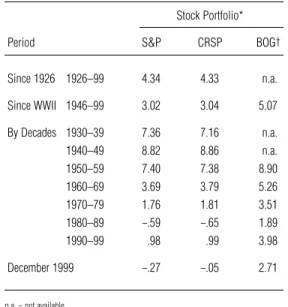
From Chart 4 and Table 2, we can see that average stock yields during the 1960s and the 1990s are about the same. However, the equity premium must be much smaller during the 1990s because the bond yields are higher then. Chart 5 and Table 3 display our estimates of the equity premium itself. For two of our stock portfolios (the S&P and CRSP stocks), the equity premium is actually negative during the 1980s and close to zero during the 1990s.

Recall that under the assumption of perfect capital mar-kets, economic theory justifies only a small equity premi-um (in the range of from 0 to 0.25 of a percentage point). As can be seen from Chart 5 and Table 3, our estimated premium is much larger than that for most of the 1926–99 sample period. Recently, however, the premium has shrunk to a size closer to that which theory predicts.

Between 1926 and 1970, for example, the average pre-mium for the S&P stocks relative to long-term government bonds is 6.8 percentage points. Since then, this premium has averaged 0.7 of a percentage point. In 1999, the divi-dend yield is 1.36 percent, and the bond yield is 6.82 per-cent. If we add the average S&P dividend growth rate to the S&P dividend yield and subtract the long-term bond yield, we have

(5) re9 p

9=

(

1.36percent+ 5.19percent)− 6.82percent = −0.27of a percentage point

or an equity premium that is slightly negative.

If we use the CRSP portfolio, then the equity premium is close to zero (−0.05 of a percentage point) in 1999.

For the total stocks held by U.S. residents, as measured by our BOG stock portfolio, the decrease in the equity premium has been less dramatic because of the recent growth in dividends. Between 1946 and 1970, these stock yields are 7.5 percentage points higher than bond yields on average. After 1970, this difference shrinks to 3.1 percent-age points. In 1999, the BOG equity premium is7 (6) re

9 p

9=

(

2.60percent+ 6.93percent

)

− 6.82percent = 2.71percentage points.

Robustness

The assumption that dividends are expected to grow at a constant rate through time may be too restrictive; after all, dividend growth rates have varied considerably across de-cades (Table 1). Therefore, we next consider alternative as-sumptions on the dividend process. We also consider the sensitivity of our results to different measures of dividends and bonds of different maturities. We try here to determine whether the apparent decline in the equity premium is due to mistaken assumptions behind our calculations. It does not appear to be; these exercises do not change our result. Is Our Dividend Growth Too Low?

We start by adjusting the dividend growth to take account of what may be higher productivity growth in the real U.S. economy. Some think that recent improvements in infor-mation technology have led to sustainable higher produc-tivity growth. (See, for example, Jovanovic and Rousseau 2000.) This “new economy” view assumes that the 1990s are much like the post–Industrial Revolution period, which enjoyed the fruits of tremendous technological advances. Higher productivity translates into higher growth in output, earnings, and dividends, which our original estimates of constant dividend growth did not capture.

But we don’t think such growth bursts are permanent. Ultimately, real growth increases are determined by growth in factors of production like labor and output per worker. And recent growth in these elements has not been impres-sive. In the 1990s, annual growth in the U.S. labor force has been roughly 1 percent—lower than in earlier years, when more women and baby boomers were entering the workforce. Similarly, productivity has grown only about 1 percent per year (Krugman 1997).

Still, suppose that the U.S. economy experienced not a permanent, but a temporary increase in growth, with the rate eventually returning to the postwar trend. Recall that

(5)

_. We can use the latest available dividend yields for BOG stocks to back out a value for rs. Doing this calculation, we find that rs= 9.86 percent. If rb= 6.82 percent, then the equity premium is 3.04 percentage points. This is a bit larger than our baseline 1999 estimate of 2.71 percentage points, but it is still much smaller than the 1946–70 av-erage of 7.5 percentage points.

As another example, consider our calculations for the S&P stocks. Earlier, we used a dividend growth rate for these stocks of 5.19 percent, which is the average growth rate in their dividends during 1927–99 (Table 1). This growth rate is significantly lower than that of GNP, which grew 6.72 percent on average over the same period. Sup-pose that we forecast future growth in S&P stock divi-dends to be more in line with average GNP growth. This would increase our estimate of the S&P-based equity pre-mium from −0.27 of a percentage point to 1.26 percentage points. (See Table 4.) But again, even adjusted for potential temporary increases in dividend growth, the estimated eq-uity premium is much smaller than the historical average. Is Our Dividend Yield Too Low?

Now we see if using different measures of dividends in our formula makes a difference to our estimates of the equity premium. In our earlier computations, we considered cash dividends only. During the 1980s, however, corporations increased the amount of their share repurchases, possibly as a way of providing a tax advantage for shareholders. Since share repurchases form a part of the total distribu-tions to shareholders, some think they should not be ig-nored when measuring dividends.

Theoretically, adding share repurchases to cash divi-dends should not change our calculated equity premium. When a broader measure of dividends—cash dividends plus share repurchases—is used in equation (4), g should be the growth rate in that broad measure. When a narrow measure of dividends—just cash—is used, then g should be the growth rate in that narrow measure. If share repur-chases are simply substitutes for cash dividends, then the level of the stock yield, and thus the size of the equity pre-mium, should be the same for both measures.

To see this, consider a simple example of Wadhwani (1999).

As a first scenario, suppose that a firm makes a steady annual profit of $1,000 and pays the entire profit as div-idends. Suppose also that the number of shares outstanding is 1,000 (which implies dividends per share equal to $1). If the discount rate rs_{on equity is 10 percent, then the} price of the stock is $10 [ps,0= d1/(r

s

−g) = 1/0.1]. Now consider a second scenario which involves repur-chasing shares. Suppose that the firm instead pays half of its $1,000 profit in dividends and half to repurchase shares. Let N_tequal the number of shares outstanding in year t. Dividends per share in t are, therefore, $500/N_t, with a

growth rate given by (8) g_t= (d_t/d_t−1) − 1

=

[

(500/N_t)

/

(500/N_t−1)

]

− 1 = (N_t−1/N_t) − 1.

In words, the rate of growth of dividends per share is equal to the rate of decline in the number of shares outstanding. Let ps,tbe the share price in year t. Because shareholders stand to get the whole profit stream regardless of the cor-porate dividend policy, it should be true that

(9) N_tp_s,t= $1,000/0.1.

If $500 is used to repurchase shares at price p_s,t, then

(10) ps,t(Nt−1−Nt) = 500.

Combining equations (9) and (10), we get (11) N_t/N_t−1= 1/1.05.

Hence, the growth rate for dividends is 5 percent per year. Without share repurchases, we compute a dividend yield of 0.10 and a dividend growth rate of 0 percent. With share repurchases, we compute a dividend yield of 0.05 and a dividend growth rate of 5 percent. In both scenarios, the initial share price is $10 and the stock yield is 10 per-cent. For the second scenario, we simply treat the share re-purchases as if they were a one-to-one substitute for divi-dends. Therefore, we should get the same equity premium whether we use the narrow or the broad measure of divi-dends.

We display in Chart 6 both of these measures of div-idend yields, calculated for the BOG stock portfolio.8_The

narrow series is the portfolio’s total dividends each year

divided by the stock market’s total value in the preceding year (as shown in Chart 2). The broad series is total div-idends less net new equity issues for both domestic

(6)

non-financial corporations and non-financial corporations, all di-vided by the stock market value in the preceding year. Net new equity issues are equal to new share issues less share repurchases. Chart 6 shows that the net new equity issues can add significantly to the volatility of payouts.

However, the levels of the narrow and broad measures of dividend yields both average 4.4 percent over the post– World War II period. The main difference between the two series is that broad dividend yields are more volatile. That makes it harder to form expectations for the broad yield and for future dividend growth rates. We thus are better off using the narrow measure of dividends in our estimate of the equity premium.

Is Our Bond Yield Too High?

All that we have left to tinker with is estimates of bond yields. The equity premium has decreased in the 1990s primarily because bond returns and yields have been dra-matically higher than average during those years. (See Chart 3.) In our calculations for the equity premium in 1999, we used a nominal bond yield of 6.82 percent, which is the yield of a 20-year U.S. Treasury bond. Is this yield too high?

It is certainly higher than the yield on bonds with shorter maturities. Over the period 1926–99, the average yield on 20-year Treasury bonds was 0.5 of a percentage point higher than the average yield on 5-year Treasury bonds. (See Chart 3.) In 1999, the 5-year bond yield was 6.5 percent, 0.3 of a percentage point below the 20-year yield. However, using this adjusted 1999 value in our for-mula doesn’t change the premium estimates much. The value would imply that re

9 p

9is 0.1 of a percentage point for the publicly traded (S&P and CRSP) stock portfolios and 3 percentage points for the total (BOG) stock portfo-lio—more or less the values we got with the longer-term bonds.

A more reasonable argument for a higher premium is based on transaction costs due to the illiquidity that in-vestors face with government securities. Costs incurred in shifting out of such securities can be as much as 0.5 of a percentage point. If we subtract that much from our bond yield estimate of about 6.8 percent, then our equity pre-mium formula gives an estimate of 0.3 of a percentage point for the publicly traded portfolios and 3.2 percentage points for the total stock portfolio. Yet, again, these es-timates are fairly close to our original eses-timates.

The Bottom Line

Thus, our exercises with alternative assumptions have not shaken our result. Adding net share repurchases to our cal-culations does not affect our equity premium estimates. Allowing for higher dividend growth does—but extraordi-nary growth in dividends is needed to get estimates close to the historical averages. Lowering bond yields also in-creases our estimates a bit, but bond yields have increased dramatically over our sample period. Taking account of large transaction costs due to illiquidity increases our es-timates only mildly.

Our bottom line is that the U.S. equity premium has declined significantly during 1970–99. We see this even when we use the higher stock yields for total stock hold-ings of U.S. residents (the BOG stock portfolio); reason-able assumptions lead to a premium of about 3 percentage points. For the stock portfolios that most people analyze—

S&P stocks and CRSP stocks—the premium is between 0 and 2 percentage points. To get a value around 2, though, we need to assume much faster dividend growth in the near term than is observed historically as well as large transaction costs for bonds.

Reasonableness

We have used the stock valuation model in equation (3) to calculate the equity premium at different points in time. The sizes of premium we computed should correspond to what investors expect to get only if their expectations about the future dividend growth rate match ours. While some may think that this is not likely, we argue that it is.

At face value, some of our estimates might not seem reasonable. For several years in our sample, our calculated equity premium is quite close to zero. For example, the premium calculated with S&P stocks is −0.26 of a per-centage point at the end of 1982 and −0.27 of a percent-age point at the end of 1999. If these estimates are indeed correct, then between 1982 and 1999, investors must have earned the same rate of return from stocks and bonds, aside from the differences between the actual dividends they received and what they expected to get from stocks. That is, $100 invested in either stocks or bonds at the end of 1982 would have about the same value at the end of 1999. Yet a look at the data seems to show something else. During 1982–99, S&P stocks earned an annualized average return of 18.35 percent, while an investment in 30-year government bonds, made at the end of 1982 and held until the end of 1999, earned an annualized average return of 11.68 percent—substantially less than the stock return. Does this mean our equity premium calculations are faulty?

No; the comparison itself is faulty. It is comparing as-sets which have different maturities. Stocks have a signifi-cantly longer life than 30-year government bonds, so these two types of assets would not necessarily have the same return over any particular period. A more appropriate asset to compare to stocks is bonds that have no maturity at all:

consol bonds with coupons that grow at the same rate that

stock dividends are expected to grow.

In our equity premium calculations, we assumed that S&P stock dividends grew at a constant rate of 5.19 per-cent per year (their average annual growth during 1927– 99). Hence, consider a consol bond that pays annual cou-pons—a first coupon of $1, paid at the end of the first year, and after that the coupons growing at 5.19 percent per year, forever. Then, at the end of 1982, with the long-term bond yield at 10.95 percent, the price of this consol bond will be $17.36. At the end of 1999, with the long-term bond yield at 6.82 percent, the bond’s price will be $145. Thus, an investment of $100 in this consol bond at the end of 1982, which is sold at the end of 1999, after having paid all the coupons in between, will earn an annualized aver-age return of 16.88 percent—a return close to the actual 18.35 percent annualized average return on S&P stocks over the period.

Why the 1.47 percentage point difference, if our equity premium estimates are close to zero for the period? By the end of 1999, the expected S&P dividend growth rate may have increased somewhat from our assumed 5.19 percent. That would increase the yield of S&P stocks and so the equity premium. We saw that, recall, when we changed

(7)

our assumption of growth in dividends from their 5.19 per-cent historical average to the 6.72 perper-cent historical av-erage growth of GNP. That changed assumption increased our premium estimate to 1.42 percentage points—which is still small, but in the range of the value calculated with the sample consol bond.

Confirmation

Our bottom line is consistent with those of several other recent studies that have compared U.S. stock and bond yields over time.

Perhaps the earliest is the study done by Blanchard (1993). He compares expected real yields on stocks and bonds during 1929–93. He computes expected yields as fitted values of regressions on a list of variables assumed to be part of investors’ information sets when expectations are made. As we do, Blanchard uses both intermediate-and long-term bonds. However, the stock portfolio he uses includes only publicly traded stocks; he does not consider the total stock portfolio reported by the Fed (BOG stocks). The results of Blanchard’s (1993) exercise are very close to ours for the S&P and CRSP portfolios. For ex-ample, the difference between the yield on S&P stocks and the yield on 20-year bonds that we display in Chart 4 is close to Blanchard’s estimates in his Figure 11. With ad-ditional data in the 1990s, we find that little has changed. The premium for publicly traded stocks has remained be-tween 0 and 2 percentage points.

More recently, Wadhwani (1999, Table 15) has com-pared real stock yields with returns on U.S. Treasury infla-tion-protected securities (TIPS). Like Blanchard (1993), Wadhwani only considers stocks that are publicly traded on the major U.S. stock exchanges. Using data through 1997, Wadhwani estimates a real stock yield of 4.9 per-cent—2.55 percent for the expected dividend yield (adjust-ed for buybacks) and 2.35 percent for the expect(adjust-ed growth in dividends. He uses a bond yield of 3.2 percent calculat-ed as the TIPS yield less the cost of illiquidity. Wadhwa-ni’s premium for 1998 is, therefore, 4.9 less 3.2, or 1.7 per-centage points.

Using data as of August 1999, Siegel (1999, p. 14) gets an even smaller premium. He estimates a real S&P stock yield of 3.3 percent, which is the sum of a 1.2 percent div-idend yield and a real divdiv-idend growth rate of 2.1 percent. This estimated stock yield falls below the August 1999 yield on TIPS bonds (3.3 vs. 4.0), producing a negative equity premium. Thus, Siegel looks for sources of dividend growth that could potentially increase his premium. He argues that nothing in the data can justify extrapolating the high historical stock yield forward. He also argues that the shrinking of the equity premium may be less significant because transaction costs have come down significantly.

Fama and French (2001) conclude as well that the eq-uity premium is shrinking, but their reasoning is based on a different type of calculation than ours. They compare stock yields (calculated as in our equation (3)) to average stock returns (calculated as the sum of the dividend yield and the growth rate of the stock price), and they find a dis-crepancy over time. These averages line up well for data between 1872 and 1949. From 1950 through 1999, how-ever, the average stock yields and returns diverge because stock prices grew much faster than dividends. Fama and French show that over the post–World War II period, the

growth in stock prices has been significantly higher than the growth in dividends. Stock returns are thus higher than the stock yields which are used to forecast returns.

Fama and French (2001) argue that this implies that in the future both stock returns and the equity premium will decrease. Consider a simple example that illustrates this argument. Suppose dividends are growing at a constant rate of 4 percent per year; the risk-free rate is 4 percent; and the equity premium starts at 7 percentage points and shrinks steadily over 50 years to 1 percentage point. When the equity premium decrease is not expected, a stock’s ini-tial price is only 44 percent of the price that will prevail when that decrease is fully expected and taken account of. By the end of the 50 years, the prices will converge to the same value regardless of whether the equity premium de-crease was expected. Hence, investors would earn a higher rate of return when the decrease is not expected than when it is (12.1 percent vs. 8.4 percent).

Whatever their approach to the issue, all of these stud-ies agree that the U.S. equity premium is currently lower than it has been historically.9These estimates seem, how-ever, to be in sharp contrast to the view of many academ-ic economists. Welch (2000, p. 514) recently asked 226 professors of finance to forecast the equity premium over different horizons. At the one-year horizon, their mean forecast was 5.8 percentage points, with a standard devia-tion of 4.5. At the five-year horizon, their mean forecast was 6.7 percentage points, with a standard deviation of 2.6. For longer horizons, their mean forecast was roughly 7 percentage points, with a standard deviation of about 2. Apparently, finance professors do not expect the equity premium to shrink.

This view is also stated clearly in standard finance text-books. Take, for example, Brealey and Myers (2000, p. 158), who describe how to estimate a return for a diversi-fied stock market portfolio. They do this by taking the current interest rate on U.S. Treasury bills plus the average equity premium over some historical time period. The pre-mium they use is 9.2 percentage points. In other words, they simply extrapolate past returns forward.

Brealey and Myers (2000) note that their result is con-sistent with security analysts’ forecasts of earnings growth. But if dividends and earnings grow at similar rates, how can we get such different estimates for the equity premi-um? The difference in estimates is due to assumptions about growth rates beyond the analysts’ forecast horizon. To get a large equity premium, we must assume that growth rates stay high forever. To get a premium as large as 9.2 percentage points, we need to assume growth rates in dividends or earnings to be significantly faster than growth rates in GNP.

To see this, consider our calculation using NIPA idends in equation (7). If we had assumed there that div-idends grow forever at 9.9 percent, then our estimate of the equity premium would have been 5.7 percentage points. Instead, we assumed that dividends grow at 9.9 percent for 5 years and then revert back to the trend growth rate of GNP. Thus, our estimate of the equity premium is 3.04 percentage points. To get the estimate up to Brealey and Myers’ 9.2 percentage points, we would need to assume nominal dividend growth of 13.2 percent per year—almost twice as fast as the growth in nominal GNP. This is an unreasonable assumption.

(8)

Concluding Remarks

Low predictions for stock returns have important impli-cations for future investments and for new financial the-ories. It is hard to rationalize a shrinking equity premium as a permanent shift in preferences. But institutional chang-es have occurred in the United Statchang-es that would rchang-esult in a permanent shift in stock returns.

One possibility not mentioned earlier is greater oppor-tunities for portfolio diversification. This idea was actually advanced by Merton (1987) before the 1990s stock price boom, and more recently, the idea has been pursued by Heaton and Lucas (2000). Merton shows that the equity premium can be substantially larger in an economy with incomplete diversification than in one with perfect capital markets. Heaton and Lucas estimate that the recent in-creased participation in stock markets can lead to as much as a 2 percentage point reduction in the equity premium and can therefore partially explain the high level of stock prices in the 1990s. This work goes only part way in ac-counting for the facts, but it seems to be going in the right direction.

*The authors benefited from discussions with António Baldaque da Silva, Urban Jermann, Narayana Kocherlakota, and Iwan Meier. The authors are particularly grateful to their editor, Kathy Rolfe.

†Also Adjunct Professor of Economics, University of Minnesota.

1_{For a discussion of indirect transaction costs, see Treynor 1994.}

2_{If, however, the decline in the equity premium and the consequent rise in equity}

prices are due to “irrational exuberance” as advocated by Shiller (2000), then investors will be even more disappointed. When the exuberance evaporates and the equity pre-mium increases to a size closer to its historical average, stock prices will fall.

3_{Note that the equity premium is sometimes defined as the expected return on}

equities in excess of the short-term interest rate. This is so in Mehra and Prescott 1985.

4_{For a brief overview of historical returns on U.S. financial assets, see the Appendix.}

Our primary data sources are Ibbotson Associates 2000 for Standard & Poor’s stock data and U.S. government bond data; the Center for Research on Security Prices (http://gsb www.uchicago.edu/research/crsp) for CRSP stock data; and FR Board, various dates, for all stocks held by U.S. residents (BOG stocks).

5_{See FR Board, various dates, Table L.213. To construct the market value of our}

BOG portfolio, we start with the total corporate issues at market value (line 1) and sub-tract from that the holdings of U.S. issues by foreign residents (line 8). We exclude the holdings of foreign residents so that we can later match up the stock values with dis-tributions paid on the stocks, which we do not have for foreigners.

6_{According to economists at the U.S. Commerce Department’s Bureau of}

Eco-nomic Analysis, the difference between NIPA dividends and dividends reported by the CRSP is attributable to differences in coverage. NIPA dividends are benchmarked to corporate tax data collected by the U.S. Internal Revenue Service. The IRS’s corporate universe in 1997 covered 4.7 million tax returns. In addition to including other public corporations which are not listed on the NYSE, AMEX, and Nasdaq, this universe in-cludes privately held corporations. A large subset of the privately held sector is the cat-egory of S corporations, which grew rapidly during the 1990s. According to the IRS, in 1997, this category accounted for 18 percent of total cash dividend distributions. Div-idend distributions from S corporations would not be included in any aggregation of public corporate data.

There is an issue about how some dividend distributions from S corporations should be categorized. If some of this income is not distributions for consumption, then we would want to recategorize that income. Doing that would imply a lower dividend yield (and thus a lower equity premium) than we report for the BOG stock portfolio.

7_{Again, if some dividend income from S corporations were excluded from our}

mea-sure of dividends, then this estimate of the equity premium would be lower.

8_{We get a similar pattern when we use data from the CRSP/COMPUSTAT Merged}

Database. The dividend yield increases significantly after 1985.

9_{Bansal and Lundblad (2000) find that the equity premium has declined around the}

world as well.

Appendix

Historical Returns on U.S. Financial Assets

In this appendix, we give an overview of historical U.S. financial asset returns. These data have motivated much of the recent asset pricing literature and serve as a useful background for those un-familiar with the U.S. experience.

The Series

The accompanying table summarizes the average historical re-turns for stocks, long-term U.S. government debt, and short-term U.S. government debt. The top panel of data in this table lists annualized compounded nominal returns for different historical time periods.*

Returns for the period 1802–1997 are taken from Siegel 1998. For 1871–1997, Siegel computed the stock returns from capitalization-weighted indexes of all stocks traded on the New York Stock Exchange (NYSE) and, starting in 1962, all stocks traded on the American Stock Exchange (AMEX) and in the Nasdaq Stock Market as well. Capitalization-weighted indexes use a firm’s stock price times shares outstanding as weights for individual firms. Before 1871, the series are based primarily on stocks of financial institutions, like banks and insurance com-panies.

Siegel’s returns on debt are returns on U.S. government se-curities, both short-term bills and long-term bonds, when avail-able. When these are not available, comparable highly rated se-curities with low default premiums are used.

After 1926, the data on most stocks and on U.S. Treasury securities are taken from Ibbotson Associates 2000. The small-firm stocks are those of small-firms in the smallest quintile of small-firms in terms of their market value of equity, as listed in the New York Stock Exchange. The S&P stocks are those in the Standard & Poor’s 500-stock price index. The Treasury bill has a 1-month maturity; the Treasury bond, a 20-year maturity. The value-weighted stock returns are taken from the data base of the Center for Research in Security Prices (CRSP). As with Siegel’s stock returns, these returns are a weighted index of all publicly traded firms on the NYSE, AMEX, and Nasdaq. The weight for each firm in a particular month is its market value (that is, its stock price times its shares outstanding) as of the previous month di-vided by the total market’s value.

The Relative Values

Consider compounded annual nominal returns over the past two centuries. In the period 1802–1997, stocks earned a premium of 4.1 percentage points over Treasury bills. In the 20th century, the premium is even larger. Take, for example, the period 1926–99. The difference in average returns on the value-weighted portfolio over Treasury bills is 7.1 percentage points—despite the fact that during this period the United States experienced both the Great Depression and World War II. Small-firm and S&P stocks both did better during 1926–99 than the value-weighted CRSP port-folio, earning a premium of 8.8 and 7.5 percentage points, re-spectively. Even during the period of the Great Depression and World War II, stocks earned a high return—higher than bills by between 6.0 and 8.3 percentage points.

In the middle panel of the table, we display standard devia-tions of the annual nominal returns. Historically, stock returns are considerably more volatile than Treasury securities—espe-cially small-firm stocks. For example, the standard deviation for small-firm stocks, which yielded the highest returns in every subperiod, is 33.6 in 1926–99, whereas the contemporaneous standard deviations for S&P stocks, Treasury bills, and Treasury bonds are 20.1, 3.2, and 9.3, respectively. The variability of Treasury bond returns increased significantly after 1970 due to

(9)

inflation uncertainty. Investors demanded a higher return on these bonds to compensate for the perceived higher risk.

In the bottom panel of the table, we report the real returns, which are the relevant numbers for investors. (These are the nominal returns, adjusted for inflation, as measured by the con-sumer price index.) Over the two centuries, the real return on the value-weighted CRSP portfolio is 7 percent while that on Trea-sury bills is only 2.9 percent. In the 20th century, the return to that short-term debt has been even lower—falling below 1 per-cent after 1926. At the same time, real returns for both small-firm and S&P stocks have been around 8 percent.

In the accompanying chart, we show graphically how the various types of financial assets have performed by plotting the changing value of $1 invested in each type in 1926. The plot is intended to further illustrate the large differences in returns across the asset types. We use a logarithmic scale for this chart because the values of the investments are vastly different.

The relative values are clear in the chart. A $1 investment in small-firm stocks in 1926 could have been cashed in for more than $6,600 in December 1999. A $1 investment in a portfolio with S&P or CRSP stocks would have turned into around $2,000 or $3,000. While not as good as the small-firm portfolio, these stock values dwarf those of Treasury securities of either maturity. A $1 investment in 20-year Treasury bonds in 1926 could have been cashed in for only about $40 at the end of 1999, and the same investment in 1-month Treasury bills could have returned only about $15.

Appendix Note

*Given nominal returns rt, t = 1, ..., T, we calculate the compounded average annual return as follows:

100{[(1+r1)(1+r2) . . . (1 + rT)]

12 / T_{− 1}_}_.

For real returns, we subtract the monthly inflation rate from rtbefore doing the cal-culation.

References

Bansal, Ravi, and Lundblad, Christian. 2000. Fundamental values and asset returns in global equity markets. Manuscript. Duke University.

Blanchard, Olivier Jean. 1993. Movements in the equity premium. Brookings Papers on Economic Activity, Macroeconomics 2: 75–118.

Brealey, Richard A., and Myers, Stewart C. 2000. Principles of corporate finance. 6th ed. Boston: McGraw-Hill.

Campbell, John Y., and Shiller, Robert J. 1988. The dividend-price ratio and expecta-tions of future dividends and discount factors. Review of Financial Studies 1 (Fall): 195–228.

Claus, James, and Thomas, Jacob. 1999. The equity risk premium is much lower than you think it is: Empirical estimates from a new approach. Manuscript. Graduate School of Business, Columbia University.

Cochrane, John H. 1997. Where is the market going? Uncertain facts and novel theories. Economic Perspectives 21 (November/December): 3–37. Research Department, Federal Reserve Bank of Chicago.

Fama, Eugene F., and French, Kenneth R. 2001. The equity premium. Working Paper 522. Center for Research in Security Prices, Graduate School of Business, Uni-versity of Chicago.

Federal Reserve Board of Governors (FR Board). Various dates. Flow of Funds Ac-counts of the United States. Statistical release Z.1. Washington, D.C.: Board of Governors of the Federal Reserve System. Available at http://www.federal reserve.gov/releases /Z1/.

Gordon, Myron J. 1962. The investment, financing, and valuation of the corporation. Homewood, Ill.: Irwin.

Hansen, Lars Peter, and Jagannathan, Ravi. 1991. Implications of security market data for models of dynamic economies. Journal of Political Economy 99 (April): 225–62.

Heaton, John, and Lucas, Deborah J. 2000. Stock prices and fundamentals. In NBER Macroeconomics Annual 1999, ed. Ben S. Bernanke and Julio Rotemberg, Vol. 14, pp. 213–42. Cambridge, Mass.: MIT Press/National Bureau of Economic Re-search.

Ibbotson Associates. 2000. Stocks, bonds, bills, and inflation—2000 yearbook. Chicago: Ibbotson Associates, Inc.

Jovanovic, Boyan, and Rousseau, Peter L. 2000. Accounting for stock market growth: 1885–1998. Manuscript. New York University.

Kocherlakota, Narayana R. 1996. The equity premium: It’s still a puzzle. Journal of Economic Literature 34 (March): 42–71.

Krugman, Paul. 1997. How fast can the U.S. economy grow? Harvard Business Review 75 (July–August): 123–29.

Mehra, Rajnish, and Prescott, Edward C. 1985. The equity premium: A puzzle. Journal of Monetary Economics 15 (March): 145–61.

Merton, Robert C. 1987. A simple model of capital market equilibrium with incomplete information. Journal of Finance 42 (July): 483–510.

Shiller, Robert J. 2000. Irrational exuberance. Princeton, N.J.: Princeton University Press.

Siegel, Jeremy J. 1998. Stocks for the long run: The definitive guide to financial market returns and long-term investment strategies. 2nd ed. New York: McGraw-Hill. ___________. 1999. The shrinking equity premium: Historical facts and future forecasts.

Journal of Portfolio Management 26 (Fall): 10–17.

Treynor, Jack L. 1994. The invisible costs of trading. Journal of Portfolio Management 21 (Fall): 71–78.

U.S. Department of Commerce, Bureau of Economic Analysis. (U.S. Commerce) Var-ious dates. National income and product accounts of the United States. Survey of Current Business. Available at http://www.bea.doc.gov.

Wadhwani, Sushil B. 1999. The U.S. stock market and the global economic crisis. Na-tional Institute Economic Review (January): 86–105.

Welch, Ivo. 2000. Views of financial economists on the equity premium and on pro-fessional controversies. Journal of Business 73 (October): 501–37.

(10)

Charts 1–2

Three U.S. Corporate Stock Portfolios Annually, 1926–99 1926 0 .2 .4 .6 .8 1.0 1.2 1.4 1.6 1.8 2.0 Ratio 1930 1940 1950 1960 1970 1980 1990 1999 1926 1930 1940 1950 1960 1970 1980 1990 1999

Chart 1 Market Value

Ratio of Each Portfolio’s Market Value to U.S. Gross National Product

Chart 2 Dividend Yield

Each Portfolio’s Dividends as a Percentage of Its Market Value*

Standard & Poor’s composite index Value-weighted index of publicly traded stocks constructed by the Center for Research in Security Prices All stocks held by U.S. residents, according to the Board of Governors of the Federal Reserve System BOG:

S&P: CRSP:

Sources: Ibbotson Associates 2000; Center for Research in Security Prices, Graduate School of Business, University of Chicago; FR Board, various dates; U.S. Commerce, various dates

*The BOG dividend yield is constructed from Federal Reserve Board market values and national income and product account dividends. 0 9 % 2 3 4 5 6 7 8 1 S&P CRSP BOG S&P CRSP BOG

(11)

Chart 3

U.S. Treasury Bond Yields

Annual Yield on Intermediate-Term (5-Year) and Long-Term (20-Year) U.S. Treasury Securities, 1926–99

1926 0 4 6 8 10 12 1930 1940 1950 1960 1970 1980 1990 1999

Source: Ibbotson Associates 2000 2

14 %

Intermediate Long

(12)

Charts 4–5 and Table 3 The U.S. Equity Premium Annually, 1926–99 1926 0 10 15 % 1930 1940 1950 1960 1970 1980 1990 1999 1926 1930 1940 1950 1960 1970 1980 1990 1999

Chart 4 Yields on Stocks and Bonds

Chart 5 Differences Between Yields on Stocks and Bonds Yield on Each Stock Portfolio* Less Yield on Long-Term Bond

*For definitions of the stock portfolios, see Charts 1–2. –4

14 % Points

Stock Yields = Each Portfolio’s* Dividend Yield + Average Growth Rate of Its Dividends

Bond Yield = Annual Yield on Long-Term (20-Year) U.S. Treasury Bonds

S&P CRSP BOG S&P CRSP BOG Bonds

Standard Model’s Prediction

0 2 4 6 8 10 12 –2 5

(13)

Chart 6

Two Measures of the Dividend Yield

Dividend Yields of the BOG Stock Portfolio* (Dividends as a Percentage of Market Value) Calculated With Share Repurchases (Broad Measure) and Without Them (Narrow Measure) Annually, 1946–99 1946 0 5 7 8 9 10 1950 1960 1970 1980 1990 1999 4 3 2 1 11 % Narrow Broad

*The BOG stock portfolio’s dividend yields are constructed from Federal Reserve Board market values and national income and product account dividends.

Sources: FR Board, various dates; U.S. Commerce, various dates 6

(14)

Table 1

Growth of U.S. Stock Dividends

Average Annual Rates of Growth in Various Periods, 1927–99

Dividends of Stock Portfolios*

Period S&P CRSP BOG†

Since 1926 1927–99 5.19 5.36 6.93 6.72 3.21 Since WWII 1946–99 6.34 6.20 8.37 7.34 4.18 By Decades 1930–39 –1.00 –1.37 .00 –.30 –1.96 1940–49 6.78 7.86 6.81 11.69 5.64 1950–59 5.15 5.53 5.98 6.69 2.07 1960–69 5.66 5.48 6.79 6.89 2.33 1970–79 5.83 7.09 9.21 10.14 7.09 1980–89 7.11 8.04 10.52 7.83 5.56 1990–99 4.72 3.24 9.19 5.37 3.01 Nominal U.S. GNP U.S. Consumer Price Index

*The stock portfolio growth rates are based on dividends per share for the S&P and CRSP stocks and on corporate dividends from the national income and product accounts for the BOG stocks. For definitions of the stock portfolios, see Charts 1–2. †These data begin in 1930.

(15)

Table 2

Yields on U.S. Stocks and Bonds Annual Averages, 1926–99

Stock Yields*

Since 1926 1926–99 9.65 9.63 n.a. 5.30 Since WWII 1946–99 9.32 9.34 11.37 6.30 By Decades 1930–39 10.33 10.12 n.a. 2.96 1940–49 11.06 11.10 n.a. 2.24 1950–59 10.51 10.49 12.01 3.11 1960–69 8.47 8.56 10.04 4.78 1970–79 9.33 9.38 11.08 7.57 1980–89 9.80 9.75 12.28 10.39 1990–99 7.83 7.84 10.84 6.85 December 1999 6.55 6.77 9.53 6.82 Bond Yields: 20-Year Treasury Bonds

n.a. = not available

*Dividends for the S&P and CRSP stocks are assumed to grow at their 1927–99 annual averages; dividends for the BOG stocks, at the 1930–99 annual average of their series. For definitions of the stock portfolios, see Charts 1–2.

†Values of the BOG stocks begin in 1946.

(16)

Table 3 Average Yield Differences Over Various Time Periods

Stock Portfolio*

Since 1926 1926–99 4.34 4.33 n.a. Since WWII 1946–99 3.02 3.04 5.07 By Decades 1930–39 7.36 7.16 n.a. 1940–49 8.82 8.86 n.a. 1950–59 7.40 7.38 8.90 1960–69 3.69 3.79 5.26 1970–79 1.76 1.81 3.51 1980–89 –.59 –.65 1.89 1990–99 .98 .99 3.98 December 1999 –.27 –.05 2.71

*For definitions of the stock portfolios, see Charts 1–2. †Values of the BOG stocks begin in 1946.

(17)

Table 4

The Recalculated U.S. Equity Premium

Average Yield Differences Between Stocks and Bonds Over Various Time Periods With Stock Yields Recalculated as the Sum of Each Portfolio’s* Dividend Yield and the Average Growth Rate of U.S. Gross National Product in 1927–99

Stock Portfolio*

Since 1926 1926–99 5.88 5.68 n.a. Since WWII 1946–99 4.55 4.39 4.86 By Decades 1930–39 8.90 8.51 n.a. 1940–49 10.35 10.21 n.a. 1950–59 8.93 8.73 8.69 1960–69 5.23 5.14 5.05 1970–79 3.30 3.16 3.30 1980–89 .94 .71 1.67 1990–99 2.51 2.35 3.77 December 1999 1.26 1.31 2.50

*For definitions of the stock portfolios, see Charts 1–2. †Values of the BOG stocks begin in 1946.

(18)

U.S. Financial Asset Returns Over the Last Two Centuries Compounded Annual Average Returns (%) on Various Stock Portfolios and on U.S. Treasury Securities, 1802–1999

U.S. Treasury

Stocks Securities

Type Type of Calculation Value- 20-Year 1-Month

of Return and Period Small-Firm S&P Weighted Bonds Bills

Compounded Average 1802–1997 n.a. n.a. 8.4 4.8 4.3 1926–99 12.6 11.3 10.9 5.1 3.8 1945–99 14.7 13.3 12.9 5.4 4.7 1926–45 9.4 7.1 6.5 4.7 1.1 1945–72 13.7 12.8 12.4 2.2 2.7 1972–99 15.4 14.1 13.6 8.7 6.8 Standard Deviation

1802–1997 n.a. n.a. 17.5 6.1 n.a.

1926–99 33.6 20.1 20.2 9.3 3.2 1945–99 25.7 16.5 16.6 10.4 3.1 1926–45 51.1 28.3 28.3 4.8 1.5 1945–72 28.5 16.6 16.5 6.0 1.8 1972–99 22.6 16.4 16.7 12.5 2.7 Compounded Average 1802–1997 n.a. n.a. 7.0 3.5 2.9 1926–99 9.3 8.0 7.5 1.9 .7 1945–99 10.1 8.8 8.4 1.1 .5 1926–45 9.4 7.1 6.4 4.6 .9 1945–72 10.2 9.3 9.0 –1.0 –.5 1972–99 9.7 8.4 8.0 3.3 1.5 Annual Nominal Returns Annual Real Returns*

*Real returns are based on changes in the U.S. consumer price index.

Sources: Siegel 1998; Ibbotson Associates 2000; Center for Research in Security Prices, Graduate School of Business, University of Chicago

(19)

The Relative Returns of U.S. Financial Assets in the 20th Century How the Value of $1 Invested in Each Type of Asset* in 1926

Would Have Changed by the End of 1999 Monthly, January 1926–December 1999

1926 .1 1 10 100 1000 10,000 $ (Log Scale) 1930 1940 1950 1960 1970 1980 1990 2000 1-Month Treasury Bills 20-Year Treasury Bonds CRSP Stocks S&P Stocks Small-Firm Stocks

*For definitions of the stock portfolios, see the accompanying text.

Sources of basic data: Ibbotson Associates 2000; Center for Research in Security Prices, Graduate School of Business, University of Chicago