Network Theory Approaches for the Analysis of Ordered Data.

(1)

Network Theory Approaches for the

Analysis of Ordered Data

Ryan Flanagan

Submitted in partial fulfilment of the requirements of the degree of

Doctor of Philosophy

School of Mathematical Sciences

Queen Mary University of London

United Kingdom

May 2020

(2)

Statement

of

Originality

I, RyanFlanagan,confirmthat theresearchincludedwithin thisthesis ismyownwork orthatwhereithasbeencarriedoutincollaborationwith, orsupported byothers,that this is duly acknowledged below and my contribution indicated. Previously published materialis alsoacknowledgedbelow.

IattestthatIhaveexercisedreasonablecaretoensurethattheworkisoriginal,anddoes nottothebestofmyknowledgebreakany UKlaw,infringeanythird party’scopyright orotherIntellectual PropertyRight, orcontain any confidentialmaterial.

Iaccept thattheCollegehastheright touseplagiarismdetection softwaretocheckthe electronicversion ofthethesis.

I confirm that this thesis hasnot been previouslysubmitted for the award of a degree bythis orany other university.

Thecopyrightofthisthesisrestswiththeauthorandnoquotationfromitorinformation derivedfrom itmaybe publishedwithout thepriorwrittenconsent oftheauthor.

Signature:

Date:

Detailsof collaborationand publications:

• Chapter 2 details joint work with Lucas Lacasa.: L. Lacasa and R. Flanagan, “Time reversibility from visibility graphs of nonstationary processes”. Physical Review E, 92(2):022817, 2015

• Chapter 3 details joint work with Lucas Lacasa: R. Flanagan and L. Lacasa. “Irreversibility of financial time series: A graph-theoretical approach”. Physics

(3)

3

Letters A, 380(20):1689-1697, 2016.

• Chapter 4 detail joint work with Lucas Lacasa, Uri Hasson, Jacopo Iacovacci, et al: U. Hasson, J. Iacovacci, B. Davis, R. Flanagan, E. Tagliazucchi, H. Laufs, and L. Lacasa. “A combinatorial framework to quantify peak/pit asymmetries in complex dynamics”. Scientific Reports, 8(1), 2018.

• Chapter 5 details joint work with Lucas Lacasa and Vincenzo Nicosia: R. Flanagan, L. Lacasa, and V. Nicosia. “On the spectral properties of Feigenbaum graphs”.

Journal of Physics A: Mathematical and Theoretical, 53(2):025702, 2020.

• Chapter 6 details joint work with Lucas Lacasa, Emma K. Towlson, Sang Hoon Lee et al: R. Flanagan, L. Lacasa, E. K. Towlson, S. H. Lee, and M. A. Porter. “Effect of antipsychotics on community structure in functional brain networks”.

(4)

Acknowledgments

I would like to thank my supervisor Lucas Lacasa for his extraordinary support, without which I would have not made it this far. I am also thankful for the support from the School of Mathematical Sciences (in particular Elisa Piccaro), the Research Degrees Office, and the EPSRC (for which this research was generously supported through DTP EP/N013492/1). I also do not forget the help from my undergraduate tutor, Frances Kirwan, and project supervisor, Mason Porter, for helping me start this journey.

I am fortunate to have a large number of friends, and a supportive family, whom I relied on during a rather turbulent time. In particular, my mother and my step father, and my father and my step mother, my two sisters, Lisa and Katy, my aunties and uncles, my friends Sam, Alex, Sumil, Lucy, Laura, Lily, Sammy, David, Filip, Abdulkadir, Scott, Neil, Satya and Carmel all provided practical support during that time. I also thank Jack Bartley for some template help. Lastly, I would like to thank Megan and Ørn for giving me a final push.

(5)

5

Abstract

Graphs are mathematical structures comprised of a set of nodes connected by edges, and network science is the application of graph theory to real world data. Networks are used as a model to analyse how entities, either individual actors, or complex systems, interact with one another.

The research here will consist of extracting networks (we will use the terms “graph” and “network” interchangeably) from ordered series, which we will focus on series ordered by time. We will either do this with the aid of the visibility graph, which is a method, based on visibility, for mapping a time series in to a graph, or through estimating the wavelet correlation, a more conventional method used in neuroscience. The aim is to describe the structure of time series and their underlying dynamical properties in graph-theoretical terms, and then using this motivation to analyse large data sets spanning several disciplines. We will describe a method, using the visibility graph, for quantifying reversibility of non-stationary processes and apply this method to a large financial data set, with the intent of ranking companies based on their irreversibility. We also use the visibility graph to develop a method which efficiently quantifies the asymmetries between minima and maxima in time series, and we then apply the method to a variety of data sets. Continuing with the theme of visibility, we study the spectral properties of visibility graphs extracted from trajectories of the logistic map undergoing a period-doubling route to chaos (known as the Feigenbaum scenario). Finally, we will use wavelet correlation to construct networks from fMRI time series, and examine community structure with the aim of differentiating between brain networks of patients with schizophrenia from control subjects. The general format throughout this thesis will start with theory, followed by extensive numerical simulations, which we can then apply the methods to real data sets.

(6)

Statement of Originality 2 Acknowledgments 4 Abstract 5 Table of Contents 6 List of Figures 10 List of Tables 15 1 Introduction 16

2 Time reversibility from visibility graphs of non-stationary processes 23

2.1 Introduction . . . 23

2.2 Measuring irreversibility using visibility graphs . . . 27

2.2.1 Preamble on stationary systems: white noise versus fully developed chaos . . . 33

2.3 Additive random walks . . . 36

2.3.1 Simple random walks . . . 36

2.3.2 Unbiased additive random walks . . . 39

2.3.3 Additive random walk with a drift . . . 43

2.3.4 Non-Markovian additive random walk. . . 43

(7)

Table of Contents 7

2.4 Multiplicative random walks . . . 45

2.5 Discussion . . . 52

3 Visibility graph irreversibility in financial time series 55 3.1 Introduction . . . 55

3.2 Methods . . . 56

3.2.1 Irreversibility and entropy production . . . 56

3.3 Data and Results . . . 57

3.3.1 Basic measures of Irreversibility . . . 58

3.3.2 Ranking Companies . . . 61

3.3.3 Assessing periods of financial reversibility . . . 64

4 Peak/pit asymmetries in visibility graph space 70 4.1 Introduction . . . 70

4.2 Methods . . . 75

4.2.1 Graph-theoretical framework for peak/pit asymmetry quantification 75 4.2.2 Visibility graphs and top-bottom VG/HVG asymmetry (∆VGA) . 77 4.2.3 Theoretical validation on synthetic processes . . . 81

4.2.4 Parametric Analysis . . . 90

4.3 Data extraction methods and visibility protocol . . . 91

4.3.1 EEG-fMRI data . . . 91

4.3.2 Calculating ∆VGA and protocols . . . 93

4.4 Results . . . 96

4.4.1 Application to fMRI . . . 96

4.4.2 Application: unsupervised clustering of financial periods . . . 98

4.4.3 Application: global daily temperature time series . . . 99

5 The spectral properties of visibility graphs: Feigenbaum graphs 102 5.1 Introduction . . . 102

(8)

5.2 From Horizontal visibility graphs to Feigenbaum Graphs . . . 103

5.2.1 Feigenbaum graphs withµ < µ∞: a simple parametrisation Fnk . . 104

5.2.2 The largen andk limits . . . 110

5.2.3 Feigenbaum graphs withµ > µ∞: Chaotic Feigenbaum graph en-sembles . . . 111

5.3 The caseµ < µ∞: Spectral properties in the period-doubling cascade . . . 112

5.3.1 A first view on the full spectrum ofFn . . . 113

5.3.2 Largest eigenvalueλmax forFn . . . 119

5.3.3 Other spectral properties ofFn: The Tree Number . . . 124

5.3.4 Largest eigenvaluesλmax forFnk . . . 126

5.3.5 Walk functions . . . 128

5.3.6 The complete spectrum ofF_nk: tridiagonaln-block Toeplitz matrices.132 5.3.7 Determinant of Feigenbaum Graphs . . . 135

5.4 µ > µ∞: Spectral properties of chaotic Feigenbaum graph ensembles . . . 140

5.4.1 Self-averaging properties ofλmax . . . 141

5.4.2 Searching spectral correlates of chaoticity . . . 142

5.4.3 Comparison with iid . . . 144

6 Community structure in functional brain networks 153 6.1 Introduction . . . 153

6.2 Data and Previous Studies . . . 156

6.3 Methods and Preliminary Computations . . . 158

6.3.1 Building the Networks . . . 158

6.3.2 Choosing a Scale and Thresholding Parameter . . . 160

6.3.3 Connectivity and Mean Local Clustering Coefficient . . . 162

6.3.4 Distance Measures . . . 165

6.3.5 Hierarchical Clustering . . . 172

(9)

Table of Contents 9

6.4.1 Inter-subject Comparisons . . . 173 6.4.2 Intra-subject Comparisons . . . 175 6.4.3 Synthesis of our Results from Hierarchical Clustering and

quanti-tative assessment . . . 180 6.5 Discussion . . . 185 6.6 Appendix: Network Component Sizes . . . 187

7 Conclusion 190

(10)

1.1 Big picture of the thesis . . . 18

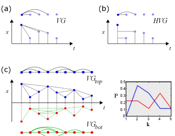
1.2 Natural visibility graph (VG) diagram . . . 20

1.3 Horizontal visibility graph (HVG) diagram . . . 21

2.1 Sample time series of an unbiased random walk. . . 25

2.2 (a) Semi-log plot degree distribution of VG for i.i.d. (b) Log-log plot of irreversibility as a function of series size nfor i.i.d. . . 35

2.3 (a) Semi-log plot of degree distribution of a time series generated from a fully chaotic logistic map. (b) Irreversibility as a function of series size n for a series generated from a fully chaotic logistic map. . . 36

2.4 (a) Log-log plot of in and out degree distributions of the VG associated to an unbiased random walk. (b) Irreversibility as a function of series size of the VG associated to an unbiased random walk. . . 42

2.5 (a) Log-log plot of in and out degree distributions of the HVG associated to an unbiased random walk. (b) Irreversibility as a function of series size of the the HVG associated to an unbiased random walk. . . 42

2.6 (a) Semi-log plot of in and out degree distributions of the HVG associated to an unbiased random walk with drift. (b) Log-log plot of irreversibility of the HVG associated to an unbiased random walk with drift. . . 44

(11)

List of Figures 11

2.7 (a) Semi-log plot of in and out degree distributions of the VG associated to a biased random walk. (b) Log-log plot of irreversibility of the VG

associated to a biased random walk. . . 45

2.8 (a) Semi-log plot of in and out degree distributions of the HVG associated to a biased random walk. (b) Log-log plot of irreversibility of the HVG associated to a biased random walk. . . 46

2.9 (a) Log-linear plot of a sample time series associated to a multiplicative random walk. (b) Log-log plot of the in and out degree distributions of a multiplicative random walk. . . 47

2.10 (a) Linear-log plot of the irreversibility measure as a function of series size n, of the VG associated to a multiplicative random walk. (b) The same plot for the HVG. . . 49

2.11 Degree distributions of the VG for multiplicative random walks of varying lengths. . . 50

2.12 (a) Log-linear plot of a sample time series associated to a multiplicative random walk. (b) Log-log plot of the in and out degree distributions of a multiplicative random walk. . . 53

2.13 (a) Log-linear plot of the irreversibility measure of the VG associated to a multiplicative random walk. (b) Log-log plot of the same measure with the HVG. . . 54

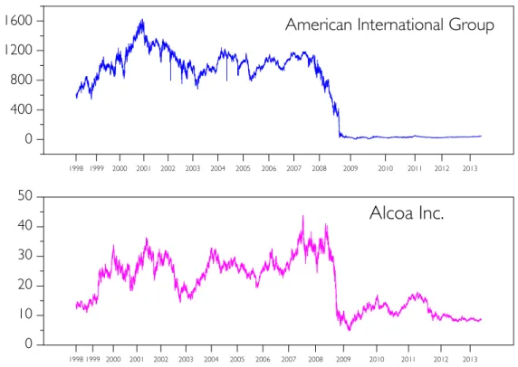
3.1 Stock prices of two companies as a function of time . . . 58

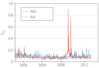
3.2 VG irreversibility of two companies as a function of time . . . 59

3.3 Scatter plot of the Score against average annualized volatility . . . 63

3.4 Scatter plot of the irreversibility variance against the irreversibility score for each company . . . 65 3.5 (a) Projection of financial periods in the PCA space of irreversibility over

15 years. (b) The same projection but based on average annualized volatility. 65 3.6 Hierarchical clustering obtained from irreversibility scores over 15 years . 67

(12)

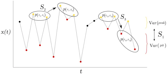
4.1 Cartoon showing the three different scenarios. . . 77 4.2 Sample time series, with corresponding top and bottom visibility and

horizontal visibility graphs for the sample time series. . . 78 4.3 Sample time series with both noisy and periodic parts. . . 79 4.4 Sample time series of white noise, chaotic logistic map and chaotic logistic

map polluted with white noise, with corresponding degree distributions for top and bottom VG and HVG. . . 81 4.5 Schematic representation of the two sets of diagrams contributing toPbot(3). 84 4.6 A few iterations of the fully chaotic logistic mapx(t+1) =F(x(t)); F(x) =

4x(1−x) . . . 85 4.7 Integrand in the last integral of Equation (4.7). . . 89 4.8 Plot of ∆VGA for a time series extracted from the logistic map with

varyingµ. . . 90 4.9 Brain regions for which the top and bottom visibility graphs differed

sig-nificantly. . . 97 4.10 Brain areas where spontaneous activity patterns differed between

wake-fulness and N2 sleep. . . 98 4.11 Relationship between variance ratio, annualized volatility and ∆VGA,

along with PCA analysis using the financial data. . . 100 4.12 PCA analysis for climate data. . . 101

5.1 Sketches of the family of infinite Feigenbaum graphs. . . 105 5.2 Single motifs F_n1 ≡Fn of the HVGs associated to the logistic maps with

period T = 2n. . . 106 5.3 A visualisation of the motif inflation (⊗) and motif concatenation (⊕) rules.106 5.4 The adjacency matrices of Fn+1 =Fn⊗Fn and Fn2 =Fn⊕Fn expressed

in terms ofAn. . . 107

5.5 A visualisation of the standard layout of F3 with its simplicial complex layout, along with equivalent nodes in red and blue. . . 109

(13)

List of Figures 13

5.6 A diagram showing the notation used in Theorem 5.3.1 . . . 113

5.7 A visualisation of the algorithm used to create a shortest path Fn, with length n. . . 117

5.8 A semilog plot of the spectrum of Fn for 0≤n≤10. . . 117

5.9 The collapse of all the spectra of Fn for varying values of n. . . 119

5.10 Compilation of bounds forλmax. . . 120

5.11 Plot of λmax(Fnk) for fixed values of nas a function of k. . . 127

5.12 Diagram of the matrix representation of (F_n2₋₁)2 in terms of the matrices An−1. . . 131

5.13 The spectrum ofF₀210. . . 133

5.14 The spectrum ofF₀210 and F₁210. . . 133

5.15 Rescaled curves forF_nk. . . 136

5.16 Diagram showingF3 with the relevant cycles. . . 137

5.17 Six other configurations for elementary spanning subgraphs ofF3. . . 138

5.18 Diagram showing each cycle’s contribution todet(Fn). . . 140

5.19 Log-log Plot showing the relative varianceRλ(N) as a function of sizeN, computed over an ensemble of 500 realisations of Feigenbaum graphs. . . 143

5.20 Scatter plot of the maximum eigenvalue λmax of F(µ,2000) vs the Lya-punov exponent le(µ), for varying µ. . . 144

5.21 Von Neumann entropy and logarithmic tree number of the Feigenbaum graph associated to a time series of N = 2000 time steps extracted from a chaotic logistic map, as a function of the map’s parameter µ. . . 145

5.22 Ensemble histogramP(λmax) for µ= 4 and i.i.d. . . 146

5.23 p-values for the 2-sampled t-test between hλµmaxi and hλiidmaxi, averaged over 50 realisations of white uniform noise and the logistic map, for varying values of µ. . . 147

5.24 Histogram showing the distribution of eigenvalues for the Feigenbaum graphs associated to the fully chaotic logistic map, versus the one associ-ated to an i.i.d. time series of the same size. . . 148

(14)

5.25 Scatter plot of the Hellinger distance between the eigenvalue distribution of Feigenbaum graphs and HVGs associated to a random i.i.d. time series of the same size as a function of the Lyapunov exponent. . . 149

6.1 Protocol of clustering brain networks gathered from fMRI data . . . 159 6.2 An array of graphs showing p-values associated to calculations related to

clustering coefficients . . . 161 6.3 Average and std for connectivity and clustering coefficient . . . 164 6.4 Connectivity of each subject under placebo. . . 164 6.5 An illustration of MRF curves, and the communities for a specific value

of γ . . . 172 6.6 Illustration of possible comparisons between the groups of subjects and

different drug treatments. . . 173 6.7 Dendrogram for the drug Aripiprazole for all subjects using a simple

dis-tance measure. . . 174 6.8 Dendrogram for the drug Aripiprazole for all subjects using the MRF

distance measure. . . 176 6.9 Dendrogram for the drug Sulpiride, and placebo. . . 176 6.10 Dendrogram for the drug Arpiprazole, vs. placebo, for the patient group. 177 6.11 Dendrogram for the drug Arpiprazole, vs. placebo, for the control group. 177 6.12 Dendrogram for the drug Sulpiride, vs. placebo, for the control group. . . 179 6.13 Dendrogram for the drug Sulpiride, vs. placebo, for the patient group. . . 179 6.14 Dendrogram for our MRF analysis of functional brain networks for our

comparison between Aripiprazole and Sulpiride for the control group. . . . 180 6.15 Dendrogram for our MRF analysis of functional brain networks for our

comparison between Aripiprazole and Sulpiride. . . 181 6.16 A cartoon illustrating purity curves. . . 183

(15)

List of Tables

3 Full list of companies with associated irreversibility score rank . . . 62

4 Summary of results across several synthetic processes. . . 92

5 Number of spanning trees in Fn. . . 126

6 Network component sizes . . . 187

(16)

Introduction

The goal of this thesis is to investigate the structure of ordered series (for example, trajectories of a dynamical system, or real world fMRI data) by developing and using new tools which originate in network and graph theory (in what follows, we will use the words graph and network interchangeably). Here we will focus on series ordered by time, but in practice all of the methods and results are relevant to any series with a suitable ordering.

In recent years we have witnessed how both the theoretical and the experimental inves-tigation of time series benefit from insights which originate in different disciplines such as graph theory and network science. Let us consider one scenario. In neuroscience it is customary to track and record brain activity by measuring the electrical activity in different regions of the brain. By installing sensors in “regions of interest” (RoIs), we can extract multivariate time series (where each entry corresponds to the electrical activity in a different RoI) which characterise the brain’s electrical activity of a subject. We can do this while this subject is performing a given task, where the default, control task is the subject at rest (which is also called “resting state”). A similar approach is used with functional magnetic resonance imaging (fMRI) data. To investigate how different regions of the brain dynamically coordinate, and to have a good picture of

(17)

Chapter 1. Introduction 17

this coordination at a global scale, it is customary to construct “functional networks”. These are graphs where each RoI corresponds to a different node in the network, and two nodes are linked by a weighted edge, where the weight corresponds to the degree of correlation or synchronisation between the two nodes (one can then turn this weighted network in to a binary network by thresholding). Once a functional network is extracted, then one can use such a network as a global descriptor of the multivariate signal. For instance, one can investigate whether the effect of a drug administered to the subject is inherited in the structure of the functional networks in a quantitative way. Similarly, one can investigate whether different psychological disorders, such as schizophrenia, can be “characterised” in such functional networks, and if so, whether these can be used for diagnoses. In Chapter 6 we will investigate how such an approach can help us to understand the effect of different antipsychotic drugs in the treatment of schizophrenia. To do that, we will first construct functional networks extracted from fMRI data and we will explore if community structures of these networks is different for control subjects (without schizophrenia) compared to patients diagnosed with schizophrenia. We will also explore whether community structure changes when each of the subject groups are treated with different antipsychotic drugs.

Another scenario where graphs and networks play a role in the description of time series is referred to as the “network based time series analysis” [1]. One can investigate the structure of a time series in graph-theoretic or combinatoric terms, with in principle two different objectives in mind: (i) a more theoretical one, where the aim is to provide a combinatorial description of certain classes of dynamics and where the objective is to produce rigorous and analytical results linking dynamical and combinatoric properties, and (ii) a more applied one, where the time series are considered as experimental ob-servations, and the aim is to use this mapping as a tool for extracting (graph-theoretic) features describing each experimental signal, and to eventually feed machine learning algorithms for statistical learning purposes.

(18)

Evolution equation

(ﬂow, map)

or

Experiment/data

(fMRI, EEG, climate) 1

1 Visibility algorithm (Ch 2, 3, 4 and 5) 2 Wavelet correlation (Ch 6) 3

or

VG analysis (Ch 2, 3, 4 and 5)

or

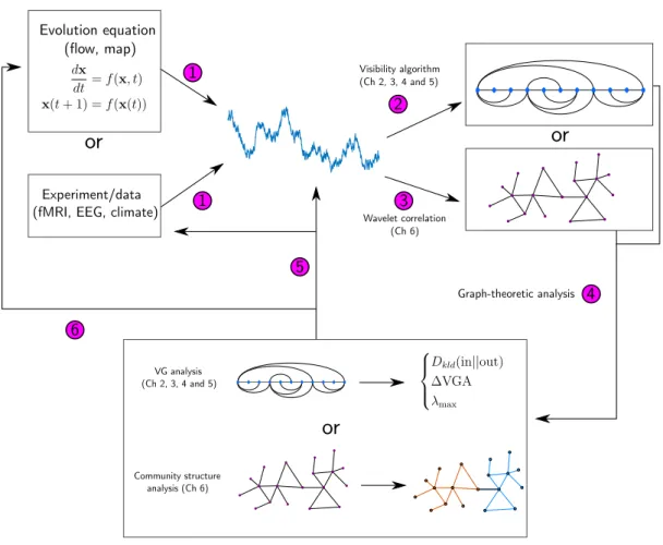
Community structure analysis (Ch 6) 4 Graph-theoretic analysis 6 5

Figure 1.1: An illustration of the big picture of this thesis. We start with step 1, generating a time series from either an evolution equation, or data. We take this time series and create a graph, either with the use of the visibility algorithm (step 2) or wavelet correlation (step 3). We then perform a graph-theoretic analysis in step 4; for VG analysis we show some example quantifiers we will use, and for the community structure analysis we show a sample network with two possible communities. We then link back to the original evolution equation or data.

having a similar aim [1]. We will use two methods. First, we will use the visibility algorithm: from a given signal x(t) one extracts a graphG= (V, E), in such a way that the topology of G inherits or encodes the structure of the time series (and, thus, the dynamical properties of the system that generated the signal). Second, we will construct correlation networks from multiple time series (each corresponding to a different RoI), using wavelet correlation. An illustration of the big picture is provided in Figure 1.1. The first step is to extract a time series. This can be, for example, a particular trajectory of a discrete dynamical system (or a sampled sequence of a continuous flow), or from a

(19)

real world experiment (such as the amount of blood flow at a region of interest, in the brain, over time). Steps 2 and 3 in Figure 1.1 consist of mapping the information stored in the time series into a graph (where step 2 involves using the visibility graph, and step 3 is using wavelet correlation) . The crucial factor is that the mapping recipe is such that the “relevant” information stored in the time series is inherited in the structure of the network, and at the same time, the “irrelevant” information is removed. Step number 4 in Figure 1.1 consists of making a graph-theoretic analysis of the resulting structure. This process is carried out by using the tools and measures of graph theory and network science to describe the structure of the graph. We will use graph properties such as the degree sequence, the degree distribution and the spectral properties of the graph. We will then link some dynamical property of the dynamical system to a topological property of the resulting graph (step 6 in Figure 1.1), as to complete the theoretical investigation. For instance, if the dynamical process is chaotic, one can aim at linking the Lyapunov exponent (a dynamical invariant) with a topological property of the resulting graph. On the other hand, if the aim is to make use of this tool for statistical learning purposes, then we can use the set of graph-theoretic descriptors as features describing the experimental signal, which can later be used in machine learning applications (step 5 in the figure). For instance, one can aim to classify whether different subjects are healthy, or have a certain condition, by projecting the signals in a space spanned by the graph theoretic features and subsequently training a classification algorithm in this space.

The visibility graph will make up the bulk of research in this thesis (more specifically, in Chapters 2 to 5), and it deserves a brief overview. The method is inspired by the concept of visibility [2] and proceeds by mapping a time series of ndata{x1, x2, . . . , xn}into an

undirected graph of n nodes according to a specific geometric criterion. As already discussed, the motivation is to subsequently make use of complex networks techniques to characterise time series. There are two types of visibility graphs: the natural visibility graph (VG) [3] and the horizontal visibility graph (HVG) [4]. In both cases, we start by constructing a vertex setV with the same cardinality of the time series n, with |V|=n.

(20)

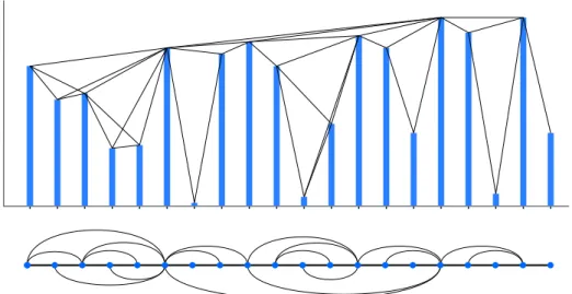
Figure 1.2: Time series (top) along with its natural visibility graph (bottom). Immedi-ately visible is the outerplanar structure and the Hamiltonian cycle

Nodes are labelled in correspondence to the time stamp of the data, i.e., node 1 is related to datum x1, node 2 is related to datum x2, and so on. However, the way nodes are linked differs between the natural and the horizontal versions of the visibility graph. In the case of the natural visibility graph, any two nodes i and j are connected if the following convexity criterion is fulfilled in the data:

xk< xi+

k−i

j−i[xj−xi], ∀k:i < k < j

Similarly, the horizontal visibility graph is a subgraph of the natural visibility graph, and is obtained by applying a similar procedure but with a slightly different, but stricter, linking criterion which instead only relies on the ordering of the data:

xk<inf{xi, xj}, ∀k:i < k < j.

It is far easier to conceptualise the algorithm if we look at a diagram, and diagrams for the natural visibility graph and horizontal visibility graph are shown in Figure 1.2 and Figure 1.3. A more thorough definition and discussion will be introduced in Chapter 2.

In this thesis we are going to extend the visibility graph methods to deal with various particular scenarios, and apply these new extensions in several applications in finance,

(21)

Figure 1.3: Time series (top) along with its horizontal visibility graph (bottom). This diagram is based upon the same time series as in Figure 1.2 and is therefore a subgraph of the natural visibility graph.

neuroscience and climate. We will also investigate purely theoretical questions.

The thesis is subsequently subdivided in a number of chapters. Each chapter aims to be self-contained, and corresponds to a different publication. Chapter 2 makes a theoretical investigation on how both the natural and horizontal visibility graphs work in the problem of detecting statistical time irreversibility, in the specific case where the dynamical process is non-stationary. The content of this chapter has been published in

Physical Review E [5]. Chapter 3 makes use of the theoretical developments of chapter

2 and applies these techniques to assess the degree of time irreversibility of financial time series. The content of this chapter has been published in Physics Letters A [6]. In Chapter 4 we extend the two version of the visibility graphs to assess the differences between maxima and minima in time series. This is carried out by considering the time series x(t), and its inverse−x(t), and analysing the difference between the degree distributions of each series’ visibility graphs. After a theoretical analysis of the methods, we showcase their performance in real-world data. The content of this chapter has been published in Scientific Reports [7]. In Chapter 5 we focus on a specific property of horizontal visibility graphs; their spectral properties. We make use of the logistic map (which generates both regular and chaotic trajectories) and make a systematic investigation of the spectral properties of the resulting graphs. The content of this

(22)

chapter has been published in Journal of Physics A [8]. Finally, in Chapter 6, we instead consider functional networks extracted from fMRI time series, and explore how these networks change when the subjects are treated with different antipsychotic drugs. The content of this chapter has been published in Journal of Complex Networks [9]. In Chapter 7 we provide a brief conclusion and discussion.

(23)

Chapter 2 Time reversibility from visibility

graphs of non-stationary

processes

2.1 Introduction

A dynamical process is stationary if its joint distribution does not change under time shift, hence sample time series extracted from the same process at different times have similar statistics, with small deviations only occurring as finite size effects. A stationary time seriesS ={x1, x2, . . . , xn} is called statistically time reversible if the series and its

time reversedS∗₌_{_x

n, xn−1, . . . , x1} are equally likely, i.e., if they have identical joint distributions [10].

For instance, Gaussian linear processes such as white noise, or conservative chaotic pro-cesses such as Hamiltonian chaos are time reversible, and related to propro-cesses in thermo-dynamic equilibrium in statistical physics. Non-linear stochastic processes, or dissipative chaotic processes are generally found to be irreversible [11], and are associated to pro-cesses that operate away from equilibrium in a thermodynamic sense. For these cases,

(24)

recent works relate the amount of entropy that a system is producing while being away from equilibrium to the amount of time irreversibility, computed from the time evolution of adequate physical observables [12].

Traditionally, the study of statistical time irreversibility has only applied to stationary processes [10]. A dynamical process is stationary if its joint distribution does not change under time shift, hence sample time series extracted from the same process at different times have similar statistics, with small deviations only occurring as finite size effects. For these processes, one can then meaningfully estimate properties about the underly-ing stationary distribution of the process (if this exists) through its estimation for finite series. In particular, one can quantify the amount of time irreversibility in stationary processes via a number of strategies and algorithms proposed in the literature, including simple statistical differences between forward and backward trajectories [11–15] or more sophisticated methods such as compression [16]. In every case, note that time series need to be symbolized before an irreversibility measure can be computed [11]. Via fluctuation theorems, a remarkable identity between the Kullback-Leibler divergence of the forward and backward statistics of a time series (i.e., the statistics ofindividual particle trajecto-ries) and the amount of entropy that the underlying thermodynamic system is producing has been found recently [12, 13], which has further stimulated the study of time series irreversibility in statistical physics. On the other hand, non-stationary processes have underlying joint distributions that change over time, hence no straightforward quantifi-cation of the time asymmetry of a process can be extracted from the analysis of finite series. The precise definition of time series reversibility in time series analysis is the following: a time series S ={x1, x2, . . . , xn} is called statistically time reversible if the

time series S−₌_{_x

−1, x−2, . . . , x−n} has the same joint distribution as S [17]. By

def-inition, non-stationary series are (infinitely) irreversible: the statistical properties of a non-stationary process vary with time, and therefore S and S− have different statistics that increase over time without bounds. It is only for stationary processes where the standard definition of time reversibility acquires its full meaning. For this latter case,

(25)

Chapter 2. Time reversibility from visibility graphs of non-stationary processes 25

x(t)

t

Figure 2.1: Sample time series of an unbiased random walk, as canonical example of a non-stationary process. By definition, the process is (infinitely) time irreversible, although if we remove the Y axis, then it is impossible to know in which direction time is flowing, as both pictures (forward and backward) are equally likely.

{x−1, x−2, . . . , x−n} and {x−1+m, x−2+m, . . . , x−n+m} have the same joint distributions ∀m, so for the particular choicem=n+ 1, the definition of time reversibility reduces to the equivalence between forward and backward statistics. Hence the popular motto “time reversibility implies stationarity” [10]. Note however, that if we understand the source of irreversibility in close relation to directionality (or, in other words, underlying sources of memory), then one could argue that there should exist different degrees of irreversibility in non-stationary processes: for instance, a Markovian random walk should arguably be “less irreversible” than a non-Markovian one, even if both are non-stationary. To further illustrate this, in Figure 2.1 we plot a realisation of a 1d random walkx(t) that starts at the origin x(0) = 0, where we have deliberately removed the vertical axis. While this is a non-stationary process and hence time irreversible, could the one assert which is the correct direction of time? Wouldn’t both the forward and backward processes be equally likely, once the vertical axis is removed? This figure could indeed both plot {x1. . . xn}

or {x−1. . . x−n}. Moreover, if x(t) describes the trajectory of a Brownian particle in a

system in thermal equilibrium, shouldn’t this time series on average have a null entropy production - hence a reversible character?

(26)

In this chapter we show that, by suitably mapping non-stationary time series into a graph-theoretical setting by means of the visibility algorithm (which we will formally define), we can actually quantify different kinds of time asymmetries in the underlying dynamics on non-stationary processes, where random walks such as the one presented in Figure 2.1 are indeed time reversible in the new framework. The family of visibil-ity algorithms were recently introduced as simple mappings between time series and graphs, with the aim of enabling the description and classification of the structure of time series as well as their underlying dynamics in graph-theoretic terms. Among other interesting advantages, these methods do not require the series to be pre-symbolized. In the context of time series irreversibility, a directed version of visibility algorithms was also proposed recently to assess irreversibility in stationary real-valued time series [18, 19], and has been used extensively [20–23]. Here we extend that former analysis to the realm of non-stationary signals. We investigate the topological properties of the visibility graphs (VGs) and horizontal visibility graphs (HVGs) associated to several types of non-stationary processes, and pay particular attention to their performance in quantifying several degrees of irreversibility. We take advantage from the fact that the topological properties of these graphs are effectively invariant under time shift for large classes of non-stationary processes, which allows us to introduce the concept of visibility graph stationarity. This in turn allows us to compare to extract meaningful information on the time asymmetry of non-stationary processes.

The rest of the chapter is as follows: in Section 2.2, we recall how univariate real-valued time series can be mapped into the family of visibility graphs (natural and horizontal versions), and explain how a directed version of these graphs can be used to estimate statistical time irreversibility of the original time series, without requiring to symbolise the series. We summarize previous findings on canonical stationary processes and prove a lemma that permits us to quantify the degree of irreversibility in non-stationary ones. In Section 2.3, we focus on random additive processes, and provide some exact results on the properties of visibility graphs associated to simple random walks. We prove that

(27)

unbiased random walks are indeed time reversible according to new definitions, and that for biased ones, the HVG method can quantify the degree of irreversibility. In Section 2.4, we extend these results to random multiplicative processes. We numerically explore the performance of visibility methods in these cases and complement these findings with some analytical and heuristic explanations. In Section 2.5 we conclude.

2.2 Measuring irreversibility using visibility graphs

Here we first introduce a formal definition of the visibility and horizontal visibility graphs associated to an ordered series of real-valued data. These are inspired in computational geometry [2] and the intuition underlying the mappings (in particular, the link criteria) shares some similarities with first passage time statistics [24]. We also introduce the notions of VG (HVG)-stationarity and VG (HVG)-irreversibility, which we will rely on subsequently.

Definition 2.2.1 (Natural Visibility Graph (VG)). Let S = {x1, . . . , xn} be a

real-valued scalar time (or otherwise ordered) series of ndata. A visibility graph (VG) is an undirected graph of nnodes, where each node i∈[1, n] is labelled by the time order of its corresponding datum xi. Hence x1 is mapped into node i = 1, x2 into node i= 2, and so on. Then, two nodes i,j (assume i < j without loss of generality) are connected by a link if and only if one can draw a straight line connecting xi and xj that does not

intersect any intermediate datum xk, i < k < j. Equivalently, i and j are connected if

the followingconvexity criterion is fulfilled:

xk< xi+

k−i

j−i[xj−xi], ∀k:i < k < j.

See Figure 1.2 in Chapter 1, for a sample time series with its respective visibility graph. By construction, VGs are planar, connected graphs, and this construction is invariant under a set of basic transformations in the series, including horizontal and vertical trans-lations. An important property of these graphs is that they are well suited to investigate

(28)

the properties of non-stationary signals. For instance, it was shown [25] that the degree distribution of VGs associated to series generated by a (non-stationary) fractional Brow-nian motion with Hurst exponent H have a power-law tail with exponent γ = 3−2H. This analysis has been subsequently applied to finance [26, 27], fluid dynamics [28, 29], and medical research [30], to cite a few. Other works applying VG to finance deal with properties such as spanning trees [31], or community structure [32].

The horizontal visibility graph is a subgraph of the natural visibility graph, and is ob-tained by applying a similar procedure but with a slightly different, but stricter, linking criterion which instead only relies on the ordering of the data:

Definition 2.2.2 (Horizontal Visibility Graph (HVG)). LetS ={x1, . . . , xn}be a

real-valued scalar time (or otherwise ordered) series of ndata. A horizontal visibility graph (HVG) is an undirected graph of n nodes, where each node i∈[1, n] is labelled by the time order of its corresponding datum xi. Hence x1 is mapped into nodei= 1, x2 into node i = 2, and so on. Then, two nodes i, j (assume i < j without loss of generality) are connected by a link if and only if one can draw a horizontal line connecting xi and

xj that does not intersect any intermediate datum xk, i < k < j. Equivalently,i and j

are connected if the following orderingcriterion is fulfilled:

xk<inf(xi, xj), ∀k:i < k < j

See Figure 1.3, in Chapter 1, for a sample time series with its respective horizontal visibility graph.

Definition 2.2.3 (VG stationarity). A dynamical process {Xt} is said to be

VG-stationary if and only if the topological properties of the VG associated to a sample time series of size nextracted from {Xt} are asymptotically (i.e., for large n) invariant

under time shift (in the statistical sense). In other words, processes for which sample time series {x1, x2, . . . , xn} and {x1+τ, x2+τ, . . . , xn+τ}, for all τ, generate (in the limit

(29)

of large n) statistically equivalent VG, are called VG-stationary. In particular, the de-gree distributions of VG associated to {x1, x2, . . . , xn} and {x1+τ, x2+τ, . . . , xn+τ} are

asymptotically (for large n) identical for VG stationary processes.

Similarly, we define HVG stationarity in the same way.

Theorem 2.2.4. Let {Xt} be a non-stationary process, and consider two time series

samples of n data extracted from{Xt}: {x1, x2, . . . , xn} and {x1+τ, x2+τ, . . . , xn+τ} for

someτ ∈_Z. If∀τ ∃c∈_Rsuch that{x1, x2, . . . , xn}and{x1+τ+c, x2+τ+c, . . . , xn+τ+c}

are statistically equivalent time series (i.e., have the same joint distributions), then the

process{Xt} is VG (HVG) stationary.

Proof. Both VG and HVG are invariant under vertical rescaling of the time series [3],

that is to say, the series S = {x1, x2, . . . , xn} and S0 = {x1 +c, x2 +c, . . . , xn+c}

generate the same VG and HVG ∀c ∈_R. Thus {x1+τ+c, x2+τ +c, . . . , xn+τ +c} and {x1+τ, x2+τ, . . . , xn+τ}also generate the same VG and HVG,∀c∈R. Choosecsuch that {x1, x2, . . . , xn} and {x1+τ +c, x2+τ +c, . . . , xn+τ +c} are statistically equivalent (i.e.,

they have identical asymptotic joint distributions). Note that in additive processes, this usually is fulfilled for c =x1 −x1+τ, but should be set for each process independently.

Then,{x1+τ+c, x2+τ+c, . . . , xn+τ+c}and{x1, x2, . . . , xn}will also generate statistically

equivalent VG and HVG, hence by definition the process is VG and HVG stationary.

Both the VG and HVG have been fruitfully applied in recent years to describe and classify different types of time series and dynamics. For instance, VG have been shown to be a viable method to quantify the Hurst exponent of fractional Brownian motion (inherently non-stationary signals); a linear relation was found between the Hurst exponent H of a time series and the exponent γ of the power law degree distribution of the associated VG,γ = 3−2H[25]. The HVG has been used in turn to describe chaotic and correlated stochastic processes [33], or to provide a graph-theoretical description of canonical routes to chaos [26, 34, 35], and it has been shown that HVGs are analytically tractable for

(30)

several classes of Markovian dynamics [36]. Both VG and HVG are connected planar graphs by construction, which have a Hamiltonian path described by the path 1−2− · · · −n. HVG are outerplanar graphs, and again by construction, one can easily prove that the HVG of S is a subgraph of VG. As both VG and HVG have a natural order induced by the time arrow (or equivalently, by the order of the associated seriesS), it is natural to define the degree sequence of a VG or a HVG as {k(t)}n

t=1, wherek(t) is the degree of nodei=t.

Note that previous definitions generate undirected graphs. However, these can be made

directed by again assigning to the links a time arrow. Accordingly, a link betweeniand

j (where time ordering yields i < j), generates an outgoing link for i and an ingoing

link for j. The degree sequence thus splits into an ingoing degree sequence {kin(t)}nt=1, where kin(t) is the ingoing degree of node i= t, and an outgoing degree sequence. An

important property at this point is that the ingoing and outgoing degree sequences are interchangeable under time series reversal. That is to say, if we define the time reversed series S∗ ₌_{_x

n+1−t}nt=1, then we have the following identities

{kin(t)}[S] ={kout(t)}[S∗]; {kout(t)}[S] ={kin(t)}[S∗] (2.1)

Now, one can define, from the ingoing and outgoing degree sequences, an ingoing degree distributionP(kin)≡Pin(k) and an outgoing degree distributionP(kout)≡Pout(k), and

property (Equation (2.1)) is inherited in the distributions, such that

Pin(k)[S] =Pout(k)[S∗]; Pout(k)[S] =Pin(k)[S∗] (2.2)

Definition 2.2.5(VG and HVG reversibility). In this thesis, a time seriesS={x(t)}n t=1 is said to be (orderp) VG-reversible (HVG-reversible) if and only if, for largen, the order p block in and out degree distribution estimates of the VG (HVG) associated to S are asymptotically identical:

(31)

Remark. According to property (Equation (2.2)), Definition 2.2.5 implies that, under the

VG/HVG setting, the statistics of the degree sequences are statistically invariant under time reversal.

Other topological properties of VG/HVG could be used to quantify time asymmetries, as has been reported recently [19]. For finite series, we will assess how close the system is to reversibility by quantifying the distance (in distributional sense) between Pin and

Pout. While several possible measures can be used, here we focus on the Kullback-Leibler

divergence between thein and outdistributions, previously proposed in [18]:

Definition 2.2.6 (Kullback-Leibler divergence or KLD).

Dkld(in||out) = X k Pin(k) log Pin(k) Pout(k)

Dkld(in||out) is a semi-distance which is null if and only if Pin(k) = Pout(k), and is

positive otherwise. As a technical remark, note that Dkld(Pin|Pout) diverges if p and q

have different supports (i.e, if q(m) = 0, p(m) 6= 0 or p(m) = 0, q(m) 6= 0 for some value m). In order to appropriately weight this possibility while maintaining a finite irreversibility measure, a common procedure is to introduce a small bias that allows for the possibility of having a small uncertainty for every contribution [13]. Here we introduce a bias of order O(1/n2) wherenis the series size (i.e. we replace all vanishing frequencies with 1/n, and we normalize the frequency histogram appropriately). We then redefine VG/HVG-reversibility as

lim

n→∞Dkld(in||out) = 0

Truly irreversible processes will have positive irreversibility values even in the limit of largen: we will call these processes VG/HVG-irreversible. For VG/HVG-reversible pro-cesses,Dkld(in||out) will have a positive finite value for finite size series that approaches

0 as size increases, withDkld(in||out)∝n−δ(whereδwill be different for VG and HVG).

(32)

com-pare and classify the degrees of reversibility of finite series across different processes, something relevant in practice.

We have checked that all the results we found in this chapter are qualitatively equiva-lent under alternative distance measures between distributions, such as the Manhattan (L1) distance DL1 = Pk|Pin(k)−Pout(k)|, although in this latter case, convergence

to zero for reversible cases is typically slower (results not shown). We also chose the Kullback-Leibler divergence one as it has some physical meaning: for stationary series, Dkld(in||out) provides a lower bound [18] to the thermodynamic entropy that a

non-equilibrium steady state described by a state variable x(t) is producing along its time evolution. Also, asindegrees account for past information whileoutdegrees account for future information (or past information in the time reversed case), then Dkld(in||out) is

formally akin toDkld(forward||backwards) in graph space, whereas orDkld(out||in) is the

formal analogue to Dkld(backwards||forward). This measure was used to assess

HVG-reversibility in the context of stationary processes and non-equilibrium steady states. Here we further extend that analysis to investigate both HVG and VG reversibility for several classes of dynamics. In what follows, we drop the specification and in the text we refer to Dkld(in||out)≡D.

In this chapter, we will mainly look at p = 1, so for readability we will drop this specification. Some important remarks are in order. First, note that there is no direct equivalence between orderpVG (HVG) reversibility in stationary processes and order p reversibility in the time series, expressed as P(x1, . . . , xp) =P(xp, . . . , x1). As a matter of fact, the degree of each node in a VG(HVG) graph inherits information from the whole time series, hence it is a global measure. Nonetheless, as we only look at orderp= 1, we can’t rule out the possibility that certain processes appear to be VG/HVG reversible at order p= 1 but are found to be irreversible at higher orders, as happens for time series produced out of equilibrium where the net current is balanced to zero via stalling forces [18]. So whereas in this chapter we are dropping the “orderp” for readability, the reader should recall that we are working at order p= 1 in the VG/HVG setting.

(33)

Second, it is important to highlight that standard methods that aim to quantify time series reversibility usually address the statistical differences of time series directly. As already stated, the original definition of time reversibility precludes the possibility of quantifying irreversibility in non-stationary signals: S = {x1, x2, . . . , xn} and S− = {x−1, x−2, . . . , x−n} have statistical differences that grow withnfor non-stationary

pro-cesses.

Third, in order to assess irreversibility directly in real-valued data, one is unavoidably required tosymbolizethe series in advance: one needs to pre-define an alphabet (with an arbitrary number of symbols) and generate a time series partition to map each datum into a symbol. Both the alphabet and the partition have to be defined ad hoc, and results often depend on these free parameters, which inevitably generates ambiguities in finite size. Furthermore, in the non-stationary realm, symbolisation is clearly ill-defined as the phase space itself grows with the series size.

Here, we take advantage of the properties of the visibility algorithms, and apply the irreversibility measures directly on the degree sequences {k(t)}T

t=1, where k(i) is the degree of node i. This sequence is discrete by construction, so there is no need to perform any ad hoc symbolisation.

2.2.1 Preamble on stationary systems: white noise versus fully

devel-oped chaos

As an illustration, let us begin by considering two paradigmatic stationary processes. The first one is white noise, a stationary and statistically time reversible uncorrelated stochastic process. Consider a sequence of i.i.d. uncorrelated random variables (i.e.,

hξ(t)ξ(t+τ)i=δ(τ)) extracted from some probability distribution p(x) with some com-pact real support as a realization of the white noise process. For this process, a theorem [18] guarantees that, asymptotically, Pin(k) =Pout(k) = 2−k and as a consequence, the

process is HVG-reversible ∀p(x). As we lack equivalent theorems for VGs, we have run numerical simulations. In Figure 2.2 we plot, in semi-log, Pin(k) andPout(k) for the VG

(34)

associated to a sample of 215 i.i.d. uniform random variables ∼U[0,1]. In panel (b) of the same figure we plot the irreversibility estimate D for increasing system size (each dot is an average over 10 realizations). We conclude that white noise is both HVG and VG-reversible showing that this process is indeed VG-reversible, in good agreement with previous theory.

For comparison, we also consider the fully chaotic logistic map xt+1 = 4xt(1−xt),

where x ∈ [0,1], a paradigmatic deterministic stationary process which is nonetheless time irreversible. HVG-irreversibility of the fully chaotic logistic map was shown in [18], where it was found that Pin(k) and Pout(k) were asymptotically different distributions.

We can summarize this by computing Pin(1) and Pout(1), and showing that they are

strictly different. We first rely on the fact that this map is Markovian, hence

Pout(k= 1) = Z 1 0 dxt Z 1 xt dxt+1f(xt)f(xt+1|xt), Pin(k= 1) = Z 1 0 dxt Z 1 xt dxt−1f(xt−1)f(xt|xt−1).

wheref(x) is the invariant probability measure that characterizes the long-term fraction of time spent by the system in the various regions of the attractor. In the case of the (fully chaotic) logistic map the attractor is the whole interval [0,1] and the invariant measure is

f(x) = 1

πpx(1−x). (2.3)

Now, for a deterministic system, the transition probability is simply

f(xt+1|xt) =δ(xt+1−F(xt)),

where δ(x) is the Dirac delta distribution and F(x) = 4x(1−x). Notice that, using the properties of the Dirac delta distribution, R1

xtδ(xt+1−F(xt))dxt+1 is equal to one

if and only if F(xt) ∈[xt,1], which happens for 0< xt<3/4, and it is zero otherwise.

Therefore the only effect of this integral is to restrict the integration range of xt to be

[0,3/4]:

Pout(k= 1) =

Z 3/4

0

(35)

Chapter 2. Time reversibility from visibility graphs of non-stationary processes 35 White noise - VG P (k ) 104 103 102 101 1 k 5 10 15 20 P_in(k) P_out(k) (a) Dkl d (i n| |o ut ) 0.001 0.01 0.1 1 n 100 1000 10000 (b)

Figure 2.2: (a) Semi-log plot of the in and out degree distributions of the natural vis-ibility graph associated to a time series of 215 i.i.d. uniformly random uncorrelated variables ∼U[0,1]. Both distributions are identical up to finite-size effects fluctuations, suggesting that the underlying process is VG-reversible. (b) Log-log plot of the irre-versibility measureDkld(in||out) as a function of the series sizen(each dot is an average

over 10 realizations). This measure vanishes asymptotically as 1/n, showing that fi-nite irreversibility values for fifi-nite size are due to statistical fluctuations that vanish asymptotically. Similarly, Pin(k= 1) = Z 1 3/4 f(xt)dxt= 1/3.

We conclude that Pout(1) 6=Pin(1) for the fully chaotic logistic map. Since D is

semi-positive definite and null if and only if the two distributions are identical, then D is strictly positive for this process, i.e., it is HVG-irreversible.

Because we don’t have equivalent theory for VGs, we have again run numerical sim-ulations for this case, which are plotted in Figure 2.3. Once again, the in and out

distributions are clearly different and their Kullback-Leibler divergence converges to a finite, positive value as the series size increases, also suggesting VG-irreversibility.

In what follows we extend previous studies on stationary signals to the realm of non-stationary time series.

(36)

Dissipative chaos - VG P (k ) 105 104 103 102 101 1 k 5 10 15 20 P_in(k) P_out(k) (a) Dkl d (i n| |o ut ) 0 0.1 0.2 0.3 n 100 1000 10000 (b)

Figure 2.3: (a) Semi-log plot of the in and out degree distributions of the natural visibility graph associated to a time series of 215 _{data generated from a fully chaotic logistic} map x(t+ 1) = 4x(t)(1−x(t)). Distributions are clearly different, suggesting that the underlying process, although stationary, is VG-irreversible. (b) Irreversibility measure Dkld(in||out) as a function of the series sizen(each dot is an average over 10 realizations).

This measure converges to a finite value with series size, confirming that the process yields a positive irreversibility measure.

2.3 Additive random walks

2.3.1 Simple random walks

Let us start by considering a simple one dimensional random walk, described by

x(t+ 1) =x(t) +ξ, ξ∈ {−1,1}, (2.4)

i.e., the step distribution is the Rademacher-1/2 distribution. Without loss of generality, if we generate a time series of n data {x1, . . . , xn} which deterministically starts in the

origin (for which E(x1) = σ2(x1) = 0), as the process is unbiased, we have E(xn) =

0 ∀n, but, in virtue of the central limit theorem, the variance fulfils σ2(xn)∼n, so the

process is non-stationary. In this subsection we derive exact results on the in/out degree distributions for this simple process.

(37)

bi-Chapter 2. Time reversibility from visibility graphs of non-stationary processes 37

infinite series generated by a 1d simple random walk are

Pin(k) =Pout(k) =        1/2 k= 1,2 0 otherwise (2.5)

Proof. First, notice that we don’t necessarily need to compute Pout(k) and Pin(k)

sepa-rately. We use property 2.5 and focus on bothPout as applied to the time series and its

time reverse, that we label Pout and Pout∗ respectively.

• k= 0: by construction there is exactly one node withkout= 0 (the final node) and

only one node with kin= 0 (the initial node), so Pout(0) =Pout∗ (0) = 1/N, where

N is the series size. Hence for bi-infinite series, Pout(0) =Pout∗ (0) = 0. • k= 1: Pout(1) = prob(xt+1≥xt) = 1/2,Pout∗ (1) = prob(xt≥xt+1) = 1/2.

• k >2: let us prove by contradiction that Pout(k >2) =Pout∗ (k >2) = 0. In order

for Pout(k > 2) > 0, there should be at least an ordering of data which allows

that a node chosen at random has degree kout >2. Let us assume that the node

associated to datum x0 is that node, which at leasthas out visibility of the node associated to x1 (by construction), xp (for some 1 < p < q) and xq (for some

q > 2). The geometrical restrictions on the data that follow from the horizontal visibility criterion are {x0 > x1; x0 > xp > x1, xq > xp}. The first restriction

yields x1 =x0−1 according to Equation (2.4). On the second condition we have xp > x1that impliesxp ≥x0. But this contradicts the first inequality of the second restriction,x0 > xp. HencePout(k >2) = 0. A similar geometrical argument yields

P_out∗ (k >2) = 0.

• Normalization of the probability yields Pout(2) =Pout∗ (2) = 1/2, which concludes

the proof.

(38)

curiosity, we will show that this is possible using simple enumerative combinatoric ar-guments. We start by using the diagrammatic approach proposed in [36], which divides the computation of each degree probability into an infinite sum of corrections of order α,Pout(2) =P∞α=0P

(α)

out(2), whereα is the number of hidden variables (hidden data) in

a given configuration. That is to say, P_out(α)(2) gathers the contribution given by all the diagrams for which we find kout = 2, that include a total of α hidden variables (hidden

data with no visibility). For instance, for kout = 2 there is exactly one path (diagram)

at order α= 0, that can be labelled as{BT}, where B stands for a movement downhill (ξ =−1) and T stands for a single movement uphill (ξ = +1). This represents the dia-gram {x0, x1, x2} where x1 =x0−1, x2 =x0, and its associated probability is directly 2−2. There are no contributing paths at order α = 1 (in fact, all odd values of α are forbidden by construction), whereas there is exactly one path at order α = 2, labelled as{BBT T}, that contributes with a probability 2−4_{. In fact, any path should start and} end by{B| · · · |T}. The number of hidden variablesα is represented here as the number of extra letters to be located. While there are a total of 2αpossible paths that start with a downhill movement and end with an uphill movement (with equal weight 2−(α+2)), not all of them are allowed in the sense of generating a valid path forkout= 2 - only strictly

negative closed walks of length α+ 2 are allowed at order α.

First, kout = 2 requires that the initial and final node have associated data of identical

height. Since the initial movement is downhill (B) and the final one is uphill (T), the hidden variables should contribute with a null vertical movement, so half of them have to be involved in a downhill movement, and half of them in an uphill one. This reduces the number of paths from 2αto _α/α₂

. Furthermore, only those paths that always remain under x0 until reaching the end datum will actually be paths of order α (if they cross thex0 level at prior stages they are considered corrections of lower order).

Interestingly, the number of allowed paths can then be seen as the number of words of length α having α/2 B’s and α/2 T’s, such that no initial segment of the word has more T’s than B’s. These paths are sometimes called Dyck words in enumerative

(39)

combinatorics. The number of Dyck words of size α is C_α/₂, where Cn is the Catalan

number Cn= 1 n+ 1 2n n

Hence Pout(2) takes the form

Pout(2) = ∞ X α=0,even C_α/₂ 1 2 α+2 = 1 4 ∞ X γ=0 1 γ+ 1 2γ γ 1 4 γ (2.6)

where we have used the change of variable γ = α/2. Leaving the pre factor 1/4 aside, (Equation (2.6)) is the generating function of the Catalan numbers evaluated atz= 1/4. The generating function sums up to [1 −√1−4z]/2z, thus Pout(2) = 1/2, in good

agreement with previous theorem.

By virtue of Theorem 2.2.4, the process described in Equation (2.4) is VG and HVG-stationary (choosingcsuch that every sample time series starts, say, a the origin, makes them statistically indistinguishable). Accordingly, one is entitled to explore the time asymmetries taking place in the graph space. According to theorem 1, as both the in and out degree distributions are equivalent for the HVG, the process is indeed HVG-reversible. We will now explore a generalization of this process and the performance of both HVG and VG.

2.3.2 Unbiased additive random walks

Let us generalize the previous simple random walk by considering an unbiased additive random walk

x(t+ 1) =x(t) +ξ, hξi= 0 (2.7)

whereξ are i.i.d. random variables extracted from some (arbitrary) symmetric distribu-tion. This process is, for instance, a (1d) discrete model of a Brownian particle evolving in an infinitely large system which is in thermodynamic equilibrium, a system which on average is not producing entropy. From a time series perspective, it is however a non-stationary process, i.e. time irreversible. The following theorem uses the VG and HVG method to somehow reconcile both aspects.

(40)

Theorem 2.3.2. A bi-infinite time series generated from the unbiased random walk

model defined in Equation (2.7) is both VG and HVG reversible.

Proof. The first step is to prove that the process described in Equation (2.7) is both VG

and HVG stationary. Choose c=x1−x1+τ in Theorem 2.2.4, for which

{x1+τ+c, x2+τ+c, . . . , xn+τ+c}={x1, x1+ (x2+τ−x1+τ), . . . , x1+ (xn+τ−x1+τ)} ={x1, x1+ξ, . . . , x1+ n−1 X i=1 ξ} ={x1, x2, . . . , xn}.

Therefore the process is VG and HVG stationary, concluding the first part of the proof.

Accordingly, reversibility reduces to investigate whether the VG/HVG of{x1, x2, . . . , xn}

and{xn, xn−1, . . . , x1}are statistically identical. To address this, we recall that visibility algorithms (both VG and HVG) are invariant under vertical rescaling [3, 4]. This means that two time series {x1, x2, . . . , xn} and {x1+c, x2+c, . . . , xn+c} yield the same VG

(and the same HVG) ∀c∈_R. In particular, the (vertically shifted) reversed time series

{xn+c, xn−1+c . . . , x1+c} and the reverse time series {xn, xn−1. . . , x1} also yield the same VG and HVG∀c∈_R. Our strategy then consists in proving that there exists a value c for which{xn+c, xn−1+c . . . , x1+c} and {x1, x2, . . . , xn} are statistically identical.

Choosec=x1−xn, for which{xn+c, xn−1+c, . . . , x1+c}={x1, x1−(xn−xn−1), x1− (ξ+xn−1−xn−2), . . .}={x1, x1−ξ, x1−P2_i₌₁ξ, . . . , x1−Pn_i₌₁−1ξ}. Note that in the last series, sinceξ has a symmetrical distribution for the process under study, then it is invariant under the transformationξ → −ξ. So{x1, x1−ξ, x1−P2i=1ξ, . . . , x1−Pni=1−1ξ} and{x1, x1+ξ, x1+Pi2=1ξ, . . . , x1+Pni=1−1ξ}are statistically equivalent. But this latter series is equivalent by definition to {x1, x2, . . . , xn}, thus concluding that the process

described in Equation (2.7) is both VG and HVG reversible.

In Figures 2.4 and 2.5, we plot the results of numerical simulations on the VG and HVG respectively, for the case of an unbiased random walk where ξ∼U[−0.5,0.5]. We

(41)

find that the in and out degree distributions of both graphs coincide (up to finite size effects), in good agreement with previous theorem. The irreversibility measure (panel b) for the HVG case decreases monotonically with series size n as O(1/n), yielding a vanishing value of irreversibility in the limit of large series. Roughly speaking, if we extend the relation between D and entropy production to the non-stationary realm, we would conclude that the process described in Equation (2.7) has a null lower bound for its entropy productiondS/dt≥Dkld(in||out) = 0, which is in good agreement with what

is expected for a system which is in thermodynamic equilibrium.

The degree distributions for the VG have a power law decay k−2, as reported in Fig-ure 2.4. While we don’t have a rigorous proof to support this, an heuristic derivation of this law can be outlined: the kout of a node i (associated to xi) chosen at random

could be heuristically approximated as Pout(k)∼#(k)q(k), where q(k) defines the time

window of the visibility basin (the average number of nodes that are ’visible’ from i). As a rough approximation,q(k) can therefore be related to the probability that the time series returns to xi after an excursion where x < xi, and this is of order k−3/2 for

un-biased random walks (the first return distribution of an unun-biased random walker). On the other hand, nodeiwon’t necessarily have outgoing visibility will all and every node within the visibility basin, but just with a fraction of them. This fraction will depend on the fluctuations (roughness) of the time series within the basin. Roughness can be quantified in terms of the series standard deviation σ, which in unbiased random walks scale like σ ∼ t1/2_{. Accordingly, the percentage of} _k _{nodes visible within the basin of} visibility should be of order k1/2/k=k−1/2. Summing up,Pout(k)∼k−3/2k−1/2∼k−2,

in good agreement with the results found in the panel (a) of Figure 2.4.

Finally, note that the finite size fluctuations decrease in VG at a slower rate than for HVG, scaling with series size as O(n−1/3). This is perhaps due to the fact that degree distributions in the VG case are power laws instead of exponential ones, thus finite size effects in this case case decay slower than for HVGs.

(42)

Non-stationary unbiased (memoryless) additive random walk - VG P (k ) 104 103 102 101 1 k 1 10 100 P_in(k) P_out(k) k-2 (a) n-1/3 Dkl d (i n| |o ut ) 0.02 0.05 0.1 0.2 0.5 n 100 1000 10000 (b)

Figure 2.4: (a) Log-log plot of the in and out degree distributions of the natural visibility graph associated to an unbiased random walk of 217 steps generated from x(t+ 1) = x(t) +ξ, whereξ ∼U[−0.5,0.5]. Both distributions are identical up to finite-size effects fluctuations, suggesting that the underlying process is VG-reversible. The distributions follow a power law tail k−2, something that can be heuristically justified according to scaling laws (see the text). (b) Log-log plot of the irreversibility measureDkld(in||out) as

a function of the series sizen(each dot is an average over 10 realizations). This measure vanishes asymptotically asn−1/3, suggesting that, although it is a non-stationary process, it is VG-reversible.

Non-stationary unbiased (memoryless) additive random walk - HVG

P (k ) 105 104 103 102 101 1 k 2 4 6 8 10 12 P_in(k) P_out(k) (a) Dkl d (i n| |o ut ) 104 103 102 101 n 100 1000 10000 (b)

Figure 2.5: (a) Semi-log plot of the in and out degree distributions of the horizontal visibility graph associated to an unbiased random walk of 217 steps generated from x(t+ 1) =x(t) +ξ, whereξ∼U[−0.5,0.5]. Both distributions are identical up to finite-size effects fluctuations, suggesting that the underlying process is HVG-reversible. (b) Log-log plot of the irreversibility measureDkld(in||out) as a function of the series size n

(each dot is an average over 10 realizations). This measure vanishes asymptotically as n−1_{, certifying that, albeit being a non-stationary process, it is HVG-reversible.}

(43)

2.3.3 Additive random walk with a drift

In this subsection we explore the effect of adding a positive drift to an additive random walk. For that purpose, we bias Equation (2.7) by defining its increments as having a small positive mean:

x(t+ 1) =x(t) +ξ, hξi>0

Note that this process is equivalent to superposing a linear trend, with positive slope

hξi to the unbiased additive random walk described in Equation (2.7). Since the VG is invariant under addition of linear trends [3], the VG associated to an unbiased random walk and a random walk with a linear trend is the same, so again this process VG-reversible (of course, by symmetry something similar happens in the case of a negative drift hξi < 0). Now, the HVG is not invariant under such transformation. Since the process is again VG and HVG stationary (choose c =x1−x1+τ in Theorem 2.2.4), we

should in principle be able to detect and quantify this additional source of irreversibility within the HVG setting. In Figure 2.6 we detail the numerical results for the HVG, for a concrete case where ξ ∼[−0.4,0.6], hξi= 0.1. The process is HVG-irreversible. As the method provides a finite positive irreversibility value that converges to limn→∞D≈7.5·

10−3, time asymmetry for this non-stationary process can be quantitatively distinguished from the unbiased case, for both finite and infinite size series. Extending again the analogy between irreversibility and entropy production to the non-stationary realm, the HVG method would provide in this case a tighter bound dS/dt ≥Dkld(in||out) ≈7.5·

10−3.

2.3.4 Non-Markovian additive random walk.

Finally, let us consider the following generalization of a random walk:

xt+1 =        xt+ξ if p > r xt−τ if p < r (2.8)