HAL Id: hal-02142661
https://hal.archives-ouvertes.fr/hal-02142661v3
Submitted on 10 Feb 2020
HAL
is a multi-disciplinary open access
archive for the deposit and dissemination of
sci-entific research documents, whether they are
pub-lished or not. The documents may come from
teaching and research institutions in France or
abroad, or from public or private research centers.
L’archive ouverte pluridisciplinaire
HAL, est
destinée au dépôt et à la diffusion de documents
scientifiques de niveau recherche, publiés ou non,
émanant des établissements d’enseignement et de
recherche français ou étrangers, des laboratoires
publics ou privés.
Screening Sinkhorn Algorithm for Regularized Optimal
Transport
Mokhtar Z. Alaya, Maxime Berar, Gilles Gasso, Alain Rakotomamonjy
To cite this version:
Mokhtar Z. Alaya, Maxime Berar, Gilles Gasso, Alain Rakotomamonjy. Screening Sinkhorn
Algo-rithm for Regularized Optimal Transport. Advances in Neural Information Processing Systems, 2019,
Vancouver, Canada. �hal-02142661v3�
Screening Sinkhorn Algorithm for Regularized
Optimal Transport
Mokhtar Z. Alaya
LITIS EA4108 University of Rouen Normandy
Maxime Bérar
LITIS EA4108 University of Rouen Normandy
Gilles Gasso
LITIS EA4108
INSA, University of Rouen Normandy
Alain Rakotomamonjy
LITIS EA4108 University of Rouen Normandy and Criteo AI Lab, Criteo Paris
Abstract
We introduce in this paper a novel strategy for efficiently approximating the Sinkhorn distance between two discrete measures. After identifying neglectable components of the dual solution of the regularized Sinkhorn problem, we propose to screen those components by directly setting them at that value before entering the Sinkhorn problem. This allows us to solve a smaller Sinkhorn problem while ensuring approximation with provable guarantees. More formally, the approach is based on a new formulation ofdual of Sinkhorn divergence problemand on the KKT optimality conditions of this problem, which enable identification of dual components to be screened. This new analysis leads to the SCREENKHORN algorithm. We illustrate the efficiency of SCREENKHORNon complex tasks such as dimensionality reduction and domain adaptation involving regularized optimal transport.
1
Introduction
Computing optimal transport (OT) distances between pairs of probability measures or histograms, such as the earth mover’s distance (Werman et al., 1985; Rubner et al., 2000) and Monge-Kantorovich or Wasserstein distance (Villani, 2009), are currently generating an increasing attraction in different machine learning tasks (Solomon et al., 2014; Kusner et al., 2015; Arjovsky et al., 2017; Ho et al., 2017), statistics (Frogner et al., 2015; Panaretos and Zemel, 2016; Ebert et al., 2017; Bigot et al., 2017; Flamary et al., 2018), and computer vision (Bonneel et al., 2011; Rubner et al., 2000; Solomon et al., 2015), among other applications (Kolouri et al., 2017; Peyré and Cuturi, 2019). In many of these problems, OT exploits the geometric features of the objects at hand in the underlying spaces to be leveraged in comparing probability measures. This effectively leads to improved performance of methods that are oblivious to the geometry, for example the chi-squared distances or the Kullback-Leibler divergence. Unfortunately, this advantage comes at the price of an enormous computational cost of solving the OT problem, that can be prohibitive in large scale applications. For instance, the OT between two histograms with supports of equal sizencan be formulated as a linear programming problem that requires generally superO(n2.5)(Lee and Sidford, 2014) arithmetic operations, which
is problematic whennbecomes larger.
A remedy to the heavy computation burden of OT lies in a prevalent approach referred to as regularized OT (Cuturi, 2013) and operates by adding an entropic regularization penalty to the original problem.
Such a regularization guarantees a unique solution, since the objective function is strongly convex, and a greater computational stability. More importantly, this regularized OT can be solved efficiently with celebrated matrix scaling algorithms, such as Sinkhorn’s fixed point iteration method (Sinkhorn, 1967; Knight, 2008; Kalantari et al., 2008).
Several works have considered further improvements in the resolution of this regularized OT problem. A greedy version of Sinkhorn algorithm, called Greenkhorn Altschuler et al. (2017), allows to select and update columns and rows that most violate the polytope constraints. Another approach based on low-rank approximation of the cost matrix using the Nyström method induces the Nys-Sink algorithm (Altschuler et al., 2018). Other classical optimization algorithms have been considered for approximating the OT, for instance accelerated gradient descent (Xie et al., 2018; Dvurechensky et al., 2018; Lin et al., 2019), quasi-Newton methods (Blondel et al., 2018; Cuturi and Peyré, 2016) and stochastic gradient descent (Genevay et al., 2016; Abid and Gower, 2018).
In this paper, we propose a novel technique for accelerating the Sinkhorn algorithm when computing regularized OT distance between discrete measures. Our idea is strongly related to a screening strategy when solving aLassoproblem in sparse supervised learning (Ghaoui et al., 2010). Based on the fact that a transport plan resulting from an OT problem is sparse or presents a large number of neglectable values (Blondel et al., 2018), our objective is to identify the dual variables of an approximate Sinkhorn problem, that are smaller than a predefined threshold, and thus that can be safely removed before optimization while not altering too much the solution of the problem. Within this global context, our contributions are the following:
• From a methodological point of view, we propose a new formulation of the dual of the Sinkhorn divergence problem by imposing variables to be larger than a threshold. This formulation allows us to introduce sufficient conditions, computable beforehand, for a variable to strictly satisfy its constraint, leading then to a “screened” version of the dual of Sinkhorn divergence.
• We provide some theoretical analysis of the solution of the “screened” Sinkhorn divergence, showing that its objective value and the marginal constraint satisfaction are properly controlled as the number of screened variables decreases.
• From an algorithmic standpoint, we use a constrained L-BFGS-B algorithm (Nocedal, 1980; Byrd et al., 1995) but provide a careful analysis of the lower and upper bounds of the dual variables, resulting in a well-posed and efficient algorithm denoted as SCREENKHORN.
• Our empirical analysis depicts how the approach behaves in a simple Sinkhorn divergence computation context. When considered in complex machine learning pipelines, we show that SCREENKHORNcan lead to strong gain in efficiency while not compromising on accuracy.
The remainder of the paper is organized as follow. In Section 2 we briefly review the basic setup of regularized discrete OT. Section 3 contains our main contribution, that is, the SCREENKHORN algorithm. Section 4 is devoted to theoretical guarantees for marginal violations of SCREENKHORN. In Section 5 we present numerical results for the proposed algorithm, compared with the state-of-art Sinkhorn algorithm as implemented in Flamary and Courty (2017). The proofs of theoretical results are postponed to the supplementary material as well as additional empirical results.
Notation.For any positive matrixT ∈Rn×m, we define its entropy asH(T) =−P
i,jTijlog(Tij).
Let r(T) = T1m ∈ Rn and c(T) = T>1n ∈ Rm denote the rows and columns sums of T
respectively. The coordinatesri(T)andcj(T)denote thei-th row sum and thej-th column sum of T, respectively. The scalar product between two matrices denotes the usual inner product, that is
hT, Wi=tr(T>W) =P
i,jTijWij,whereT
>is the transpose ofT. We write1(resp.0) the vector having all coordinates equal to one (resp. zero).∆(w)denotes the diag operator, such that ifw∈Rn,
then∆(w) = diag(w1, . . . , wn) ∈ Rn×n. For a set of indicesL = {i1, . . . , ik} ⊆ {1, . . . , n}
satisfyingi1<· · · < ik,we denote the complementary set ofLbyL{={1, . . . , n}\L. We also
denote|L|the cardinality ofL. Given a vectorw∈Rn, we denotewL = (wi1, . . . , wik)
> ∈ Rk
and its complementarywL{ ∈ Rn−k. The notation is similar for matrices; given another subset
of indicesS ={j1, . . . , jl} ⊆ {1, . . . , m}withj1 <· · · < jl,and a matrixT ∈Rn×m, we use
T(L,S), to denote the submatrix ofT, namely the rows and columns ofT(L,S)are indexed byLand
Srespectively. When applied to matrices and vectors,and(Hadamard product and division) and exponential notations refer to elementwise operators. Given two real numbersaandb, we write
2
Regularized discrete OT
We briefly expose in this section the setup of OT between two discrete measures. We then consider the case when those distributions are only available through a finite number of samples, that is
µ=Pn
i=1µiδxi∈Σnandν =
Pm
j=1νiδyj ∈Σm, whereΣnis the probability simplex withnbins, namely the set of probability vectors inRn+, i.e.,Σn ={w∈Rn+:
Pn
i=1wi= 1}.We denote their
probabilistic couplings set asΠ(µ, ν) ={P ∈Rn×m
+ , P1m=µ, P>1n=ν}.
Sinkhorn divergence. Computing OT distance between the two discrete measuresµandνamounts to solving a linear problem (Kantorovich, 1942) given by
S(µ, ν) = min
P∈Π(µ,ν)hC, Pi,
whereP = (Pij)∈Rn×mis called the transportation plan, namely each entryPijrepresents the
fraction of mass moving fromxi toyj, andC = (Cij) ∈ Rn×m is a cost matrix comprised of
nonnegative elements and related to the energy needed to move a probability mass fromxitoyj.
The entropic regularization of OT distances (Cuturi, 2013) relies on the addition of a penalty term as follows:
Sη(µ, ν) = min
P∈Π(µ,ν){hC, Pi −ηH(P)}, (1)
whereη >0is a regularization parameter. We refer toSη(µ, ν)as theSinkhorn divergence(Cuturi,
2013).
Dual of Sinkhorn divergence. Below we provide the derivation of the dual problem for the regularized OT problem (1). Towards this end, we begin with writing its Lagrangian dual function:
L(P, w, z) =hC, Pi+ηhlogP, Pi+hw, P1m−µi+hz, P>1n−νi.
The dual of Sinkhorn divergence can be derived by solvingminP∈
Rn×m+ L(P, w, z). It is easy
to check that objective functionP 7→ L(P, w, z)is strongly convex and differentiable. Hence, one can solve the latter minimum by setting∇PL(P, w, z)to0n×m. Therefore, we getPij? =
exp − 1
η(wi+zj+Cij)−1
,for alli= 1, . . . , nandj = 1, . . . , m. Plugging this solution, and setting the change of variablesu=−w/η−1/2andv=−z/η−1/2, the dual problem is given by
min
u∈Rn,v∈Rm
Ψ(u, v) :=1>nB(u, v)1m− hu, µi − hv, νi , (2)
whereB(u, v) := ∆(eu)K∆(ev)andK:=e−C/ηstands for the Gibbs kernel associated to the cost
matrixC. We refer to problem (2) as thedual of Sinkhorn divergence. Then, the optimal solutionP?
of the primal problem (1) takes the formP?= ∆(eu?
)K∆(ev?
)where the couple(u?, v?)satisfies:
(u?, v?) = argmin u∈Rn,v∈Rm
{Ψ(u, v)}.
Note that the matrices ∆(eu?
)and∆(ev?
)are unique up to a constant factor (Sinkhorn, 1967). Moreover,P? can be solved efficiently by iterative Bregman projections (Benamou et al., 2015)
referred to as Sinkhorn iterations, and the method is referred to as SINKHORNalgorithm which, recently, has been proven to achieve a near-O(n2)complexity (Altschuler et al., 2017).
3
Screened dual of Sinkhorn divergence
0 100 200 300 400 500 0.0020 0.0025 eu? ev? αu αv Figure 1: Plots of(eu? , ev? ) with(u?, v?)is the pair
solu-tion of dual of Sinkhorn diver-gence (2) and the thresholds
αu, αv. Motivation. The key idea of our approach is motivated by the
so-calledstatic screening test(Ghaoui et al., 2010) in supervised learning, which is a method able to safely identify inactive features, i.e., features that have zero components in the solution vector. Then, these inactive features can be removed from the optimization prob-lem to reduce its scale. Before diving into detailed algorithmic analysis, let us present a brief illustration of how we adapt static screening test to the dual of Sinkhorn divergence. Towards this end, we define the convex setCr
Cr
α={w∈Rr:ewi ≥α}. In Figure 1, we plot(eu
?
, ev? )where (u?, v?)is the pair solution of the dual of Sinkhorn divergence (2)
in the particular case of: n = m = 500, η = 1, µ = ν = n11n, xi ∼ N((0,0)>,(1 00 1)), yj ∼ N((3,3)>, −10.8−0.81
)and the cost matrixCcorresponds to the pairwise euclidean distance, i.e.,
Cij=kxi−yjk2. We also plot two lines corresponding toeu
?
≡αuandev
?
≡αvfor someαu>0
andαv>0, choosing randomly and playing the role of thresholds to select indices to be discarded.
If we are able to identify these indices before solving the problem, they can be fixed at the thresholds and removed then from the optimization procedure yielding an approximate solution.
Static screening test. Based on this idea, we define a so-calledapproximate dual of Sinkhorn divergence min u∈Cn ε κ ,v∈Cm εκ Ψκ(u, v) :=1>nB(u, v)1m− hκu, µi − h v κ, νi , (3)
which is simply a dual of Sinkhorn divergence with lower-bounded variables, where the bounds are
αu=εκ−1andαv=εκwithε >0andκ >0being fixed numeric constants which values will be
clear later. The new formulation (3) has the form of(κµ, ν/κ)-scaling problem under constraints on the variablesuandv. Those constraints make the problem significantly different from the standard scaling-problems (Kalantari and L.Khachiyan, 1996). We further emphasize thatκplays a key role in our screening strategy. Indeed, withoutκ,euandev can have inversely related scale that may
lead in, for instanceeubeing too large andevbeing too small, situation in which the screening test
would apply only to coefficients ofeuorevand not for both of them. Moreover, it is clear that the
approximate dual of Sinkhorn divergence coincides with the dual of Sinkhorn divergence (2) when
ε= 0andκ= 1. Intuitively, our hope is to gain efficiency in solving problem (3) compared to the original one in Equation (2) by avoiding optimization of variables smaller than the threshold and by identifying those that make the constraints active. More formally, the core of the static screening test aims at locating two subsets of indices(I, J)in{1, . . . , n} × {1, . . . , m}satisfying: eui >
αu, andevj > αv, for all(i, j)∈I×J andeui0 =αu, andevj0 =αv, for all(i0, j0)∈I{×J{,
namely(u, v) ∈ Cn αu× C
m
αv. The following key result states sufficient conditions for identifying variables inI{andJ{.
Lemma 1. Let(u∗, v∗)be an optimal solution of problem(3). Define
Iε,κ= i= 1, . . . , n:µi≥ ε2 κri(K) , Jε,κ= j= 1, . . . , m:νj ≥κε2cj(K) (4)
Then one haseu∗i =εκ−1andev∗j =εκfor alli∈I{
ε,κandj∈Jε,κ{ .
Proof of Lemma 1 is postponed to the supplementary material. It is worth to note that first order optimality conditions applied to(u∗, v∗)ensure that ifeu∗i > εκ−1theneu∗i(Kev∗)
i =κµiand if ev∗j > εκthenevj∗(K>eu∗
)j=κ−1νj, that correspond to the Sinkhorn marginal conditions (Peyré
and Cuturi, 2019) up to the scaling factorκ.
Screening with a fixed number budget of points. The approximate dual of Sinkhorn divergence is defined with respect toεandκ. As those parameters are difficult to interpret, we exhibit their relations with a fixed number budget of points from the supports ofµandν. In the sequel, we denote bynb ∈ {1, . . . , n}andmb ∈ {1, . . . , m}the number of points that are going to be optimized in
problem (3),i.e, the points we cannot guarantee thateu∗i =εκ−1andev∗j =εκ.
Let us defineξ∈Rnandζ∈
Rmto be the ordered decreasing vectors ofµr(K)andνc(K)
respectively, that isξ1 ≥ ξ2 ≥ · · · ≥ ξn andζ1 ≥ζ2 ≥ · · · ≥ ζm. To keep onlynb-budget and mb-budget of points, the parametersκandεsatisfyε2κ−1=ξnbandε
2κ=ζ mb. Hence ε= (ξnbζmb) 1/4andκ= s ζmb ξnb . (5)
This guarantees that|Iε,κ|=nband|Jε,κ|=mbby construction. In addition, when(nb, mb)tends
to the full number budget of points(n, m), the objective in problem (3) converges to the objective of dual of Sinkhorn divergence (2).
We are now in position to formulate the optimization problem related to the screened dual of Sinkhorn. Indeed, using the above analyses, any solution(u∗, v∗)of problem (3) satisfieseu∗
i ≥εκ−1and ev∗j ≥εκfor all(i, j)∈(I ε,κ×Jε,κ),andeu ∗ i =εκ−1andev ∗ j =εκfor all(i, j)∈(I{ ε,κ×Jε,κ{ ).
Hence, we can restrict the problem (3) to variables inIε,κandJε,κ. This boils down to restricting the
constraints feasibilityCn
ε κ ∩ C
m
εκto the screened domain defined byUsc∩ Vsc, Usc={u∈Rnb:euIε,κ ε
κ1nb}andVsc={v∈R
mb:evJε,κ εκ1
mb}
where the vector comparisonhas to be understood elementwise. And, by replacing in Equation (3), the variables belonging to(I{
ε,κ×Jε,κ{ )byεκ−1andεκ, we derive thescreened dual of Sinkhorn
divergence problemas min u∈Usc,v∈Vsc {Ψε,κ(u, v)} (6) where Ψε,κ(u, v) = (euIε,κ)>K(Iε,κ,Jε,κ)e vJε,κ +εκ(euIε,κ)>K (Iε,κ,Jε,κ{ )1mb+εκ −11> nbK(Iε,κ{ ,Jε,κ)e vJε,κ −κµ>Iε,κuIε,κ−κ −1ν> Jε,κvJε,κ+ Ξ withΞ =ε2P i∈I{ε,κ,j∈J{ε,κKij−κlog(εκ−1)Pi∈I{ε,κµi−κ−1log(εκ)Pj∈J{ε,κνj.
The above problem uses only the restricted partsK(Iε,κ,Jε,κ), K(Iε,κ,Jε,κ{ ),andK(I{ε,κ,Jε,κ)of the Gibbs kernelKfor calculating the objective functionΨε,κ. Hence, a gradient descent scheme will
also need only those rows/columns ofK. This is in contrast to Sinkhorn algorithm which performs alternating updates of all rows and columns ofK. In summary, SCREENKHORNconsists of two steps: the first one is a screening pre-processing providing the active setsIε,κ,Jε,κ. The second one consists
in solving Equation (6) using a constrained L-BFGS-B (Byrd et al., 1995) for the stacked variable
θ= (uIε,κ, vJε,κ).Pseudocode of our proposed algorithm is shown in Algorithm 1. Note that in practice, we initialize the L-BFGS-B algorithm based on the output of a method, called RESTRICTED SINKHORN(see Algorithm 2 in the supplementary), which is a Sinkhorn-like algorithm applied to the active dual variablesθ= (uIε,κ, vJε,κ).While simple and efficient, the solution of this RESTRICTED SINKHORNalgorithm does not satisfy the lower bound constraints of Problem (6) but provide a good candidate solution. Also note that L-BFGS-B handles box constraints on variables, but it becomes more efficient when these box bounds are carefully determined for problem (6). The following proposition (proof in supplementary material) expresses these bounds that are pre-calculated in the initialization step of SCREENKHORN.
Proposition 1. Let(usc, vsc)be an optimal pair solution of problem(6)andK
min= min
i∈Iε,κ,j∈Jε,κ
Kij.
Then, one has
ε κ∨ mini∈Iε,κµi ε(m−mb) + maxj∈Jε,κνj nεκKmin mb ≤eusc i ≤ maxi∈Iε,κµi mεKmin , (7) and εκ∨ minj∈Jε,κνj ε(n−nb) + κmaxi∈Iε,κµi mεKmin nb ≤evscj ≤maxj∈Jε,κνj nεKmin (8)
for alli∈Iε,κandj∈Jε,κ.
4
Theoretical analysis and guarantees
This section is devoted to establishing theoretical guarantees for SCREENKHORNalgorithm. We first define the screened marginalsµsc=B(usc, vsc)1
mandνsc=B(usc, vsc)>1n.Our first theoretical
result, Proposition 2, gives an upper bound of the screened marginal violations with respect to
`1-norm.
Proposition 2. Let(usc, vsc)be an optimal pair solution of problem(6). Then one has
kµ−µsck21=O nbcκ+ (n−nb) kCk∞ η + mb √ nmcµνKmin3/2 +√m−mb nmKmin + log √ nm mbc 5/2 µν (9)
Algorithm 1:SCREENKHORN(C, η, µ, ν, nb, mb) Step 1:Screening pre-processing
1. ξ←sort(µr(K)), ζ ←sort(νc(K));//(decreasing order) 2. ε←(ξnbζmb)
1/4, κ←p
ζmb/ξnb;
3. Iε,κ← {i= 1, . . . , n:µi ≥ε2κ−1ri(K)}, Jε,κ← {j= 1, . . . , m:νj ≥ε2κcj(K)}; 4. µ←mini∈Iε,κµi,µ¯←maxi∈Iε,κµi, ν←minj∈Jε,κνi,ν¯←maxj∈Jε,κνi;
5. u←log κε∨ε(m µ −mb)+ε∨nεκKν¯minmb ,u¯←log mεKµ¯ min ; 6. v←log εκ∨ ν ε(n−nb)+ε∨mεKκµ¯minnb ,v¯←log nεKmin¯ν ; 7. θ¯←stack(¯u1nb,v¯1mb), θ←stack(u1nb, v1mb);
Step 2:L-BFGS-B solver on the screened variables 8. u(0)←log(εκ−1)1nb, v(0)←log(εκ)1mb;
9. u,ˆ vˆ←RESTRICTEDSINKHORN(u(0), v(0)),θ(0)←stack(ˆu,vˆ);
10. θ←L-BFGS-B(θ(0), θ,θ¯); 11. θu←(θ1, . . . , θnb) >, θ v←(θnb+1, . . . , θnb+mb) >; 12. usci ←(θu)iifi∈Iε,κandui←log(εκ−1)ifi∈Iε,κ{ ; 13. vjsc←(θv)j ifj ∈Jε,κandvj ←log(εκ)ifj∈Jε,κ{ ; 14. returnB(usc, vsc). and kν−νsck21=O mbc1 κ + (m−mb) kCk∞ η + nb √ nmcµνK 3/2 min +√n−nb nmKmin + log √ nm nbc 5/2 µν , (10)
wherecz=z−logz−1forz >0andcµν =µ∧νwithµ= mini∈Iε,κµiandν = minj∈Jε,κνj. Proof of Proposition 2 is presented in supplementary material and it is based on first order opti-mality conditions for problem (6) and on a generalization of Pinsker inequality (see Lemma 2 in supplementary).
Our second theoretical result, Proposition 3, is an upper bound of the difference between objective values of SCREENKHORNand dual of Sinkhorn divergence (2).
Proposition 3. Let(usc, vsc)be an optimal pair solution of problem(6)and(u?, v?)is the pair
solution of dual of Sinkhorn divergence(2). Then we have
Ψε,κ(usc, vsc)−Ψ(u?, v?) =O R(kµ−µsck1+kν−νsck1+ωκ). whereR= kCk∞ η + log (n∨m)2 nmc7µν/2 andωκ=|1−κ|kµsck1+|1−κ−1|kνsck1+|1−κ|+|1−κ−1|.
Proof of Proposition 3 is exposed in the supplementary material. Comparing to some other analysis results of this quantity, see for instance Lemma 2 in Dvurechensky et al. (2018) and Lemma 3.1 in Lin et al. (2019), our bound involves an additional termωκ(withω1= 0). To better characterize ωκ, a control of the`1-norms of the screened marginalsµscandνscare given in Lemma 2 in the
supplementary material.
5
Numerical experiments
In this section, we present some numerical analyses of our SCREENKHORNalgorithm and show how it behaves when integrated into some complex machine learning pipelines.
5.1 Setup
We have implemented our SCREENKHORNalgorithm in Python and used the L-BFGS-B of Scipy. Regarding the machine-learning based comparison, we have based our code on the ones of Python Optimal Transport toolbox (POT) (Flamary and Courty, 2017) and just replaced thesinkhorn
1.1 1.25 2 5 10 20 50 100 Decimation factor n/nb 103 102 101 100 || sc|| 1 n = m = 1000 = 0.1 = 0.5 = 1 = 10 1.1 1.25 2 5 10 20 50 100 Decimation factor mb/m 103 102 101 100 || sc|| 1 n = m = 1000 = 0.1 = 0.5 = 1 = 10 1.1 1.25 2 5 10 20 50 100 Decimation factor n/nb 0.5 1.0 1.5 2.0 2.5
Running Time Gain
n = m = 1000 = 0.1 = 0.5 = 1 = 10 1.1 1.25 2 5 10 20 50 100 Decimation factor n/nb 103 102 101 100
Relative Divergence Variation
n = m = 1000
= 0.1 = 0.5 = 1 = 10
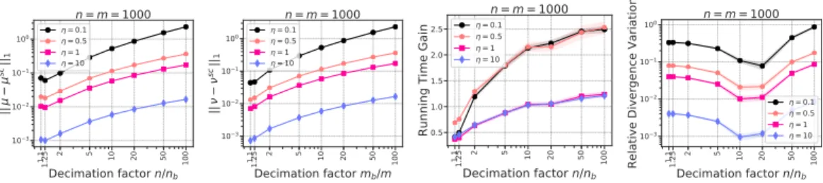
Figure 2: Empirical evaluation of SCREENKHORNvs SINKHORNfor normalized cost matrixi.e.
kCk∞ = 1. (most-lefts): marginal violations in relation with the budget of points onnandm. (center-right) ratio of computation times TSINKHORN
TSCREENKHORN and, (right) relative divergence variation. The
results are averaged over30trials.
function call with ascreenkhornone. We have considered the POT’s default SINKHORNstopping criterion parameters and for SCREENKHORN, the L-BFGS-B algorithm is stopped when the largest component of the projected gradient is smaller than10−6, when the number of iterations or the
number of objective function evaluations reach105. For all applications, we have setη= 1unless
otherwise specified.
5.2 Analysing on toy problem
We compare SCREENKHORNto SINKHORNas implemented in POT toolbox1on a synthetic example. The dataset we use consists of source samples generated from a bi-dimensional gaussian mixture and target samples following the same distribution but with different gaussian means. We consider an unsupervised domain adaptation using optimal transport with entropic regularization. Several settings are explored: different values ofη, the regularization parameter, the allowed budget nb
n =
mb
m
ranging from0.01to0.99, different values ofnandm. We empirically measure marginal violations as the normskµ−µsck
1 andkν −νsck1, running time expressed as TTSCREENKHORNSINKHORN and the relative divergence difference|hC, P?i−hC, Psci|/hC, P?ibetween S
CREENKHORNand SINKHORN, where
P?= ∆(eu?)K∆(ev?)andPsc= ∆(eusc
)K∆(evsc
).Figure 2 summarizes the observed behaviors of both algorithms under these settings. We choose to only report results forn=m= 1000as we get similar findings for other values ofnandm.
SCREENKHORNprovides good approximation of the marginalsµandν for “high” values of the regularization parameterη(η >1). The approximation quality diminishes for smallη. As expected
kµ−µsck
1andkν−νsck1converge towards zero when increasing the budget of points. Remarkably
marginal violations are almost negligible whatever the budget for highη. According to computation gain, SCREENKHORNis almost 2 times faster than SINKHORNat high decimation factorn/nb(low
budget) while the reverse holds whenn/nbgets close to 1. Computational benefit of SCREENKHORN
also depends onηwith appropriate valuesη≤1. Finally except forη= 0.1SCREENKHORNachieves a divergencehC, Piclose to the one of Sinkhorn showing that our static screening test provides a reasonable approximation of the Sinkhorn divergence. As such, we believe that SCREENKHORNwill be practically useful in cases where modest accuracy on the divergence is sufficient. This may be the case of a loss function for a gradient descent method (see next section).
5.3 Integrating SCREENKHORNinto machine learning pipelines
Here, we analyse the impact of using SCREENKHORNinstead of SINKHORNin a complex machine learning pipeline. Our two applications are a dimensionality reduction technique, denoted as Wasser-stein Discriminant Analysis (WDA), based on WasserWasser-stein distance approximated through Sinkhorn divergence (Flamary et al., 2018) and a domain-adaptation using optimal transport mapping (Courty et al., 2017), named OTDA.
WDA aims at finding a linear projection which minimize the ratio of distance between intra-class samples and distance inter-class samples, where the distance is understood in a Sinkhorn divergence sense. We have used a toy problem involving Gaussian classes with2 discriminative features
1
0 1000 2000 3000 4000 5000 Number of samples 2 4 6 8 10 12
Running Time Gain
Screened WDA on toy
dec=1.5 dec=2 dec=5 dec=10 dec=20 dec=50 dec=100 500 1000 1500 2000 2500 3000 3500 4000 Number of samples 5 10 15 20 25
Running Time Gain
Screened WDA on mnist
dec=1.5 dec=2 dec=5 dec=10 dec=20 dec=50 dec=100
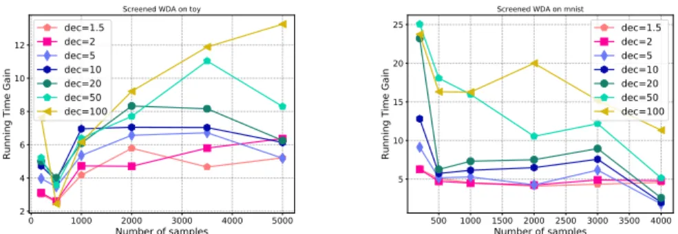
Figure 3: Wasserstein Discriminant Analysis : running time gain for (left) a toy dataset and (right) MNIST as a function of the number of examples and the data decimation factor in SCREENKHORN.
500 1000 1500 2000 2500 3000 3500 4000 Number of samples 4 6 8 10
Running Time Gain
Screened OTDA on mnist
dec=1.5 dec=2 dec=5 dec=10 dec=20 dec=50 dec=100 500 1000 1500 2000 2500 3000 3500 4000 Number of samples 4 6 8 10 12
Running Time Gain
Screened OTDA on mnist
dec=1.5 dec=2 dec=5 dec=10 dec=20 dec=50 dec=100
Figure 4: OT Domain adaptation : running time gain for MNIST as a function of the number of examples and the data decimation factor in SCREENKHORN. Group-lasso hyperparameter values (left)1. (right)10.
and8 noisy features and the MNIST dataset. For the former problem, we aim at find the best two-dimensional linear subspace in a WDA sense whereas for MNIST, we look for a subspace of dimension20starting from the original728dimensions. Quality of the retrieved subspace are evaluated using classification task based on a1-nearest neighbour approach.
Figure 3 presents the average gain (over30trials) in computational time we get as the number of examples evolve and for different decimation factors of the SCREENKHORNproblem. Analysis of the quality of the subspace have been deported to the supplementary material (see Figure 6), but we can remark a small loss of performance of SCREENKHORNfor the toy problem, while for MNIST, accuracies are equivalent regardless of the decimation factor. We can note that the minimal gains are respectively2and4.5for the toy and MNIST problem whereas the maximal gain for4000samples is slightly larger than an order of magnitude.
For the OT based domain adaptation problem, we have considered the OTDA with`1
2,1group-lasso
regularizer that helps in exploiting available labels in the source domain. The problem is solved using a majorization-minimization approach for handling the non-convexity of the problem. Hence, at each iteration, a SINKHORN/SCREENKHORNhas to be computed and the number of iteration is sensitive to the regularizer strength. As a domain-adaptation problem, we have used a MNIST to USPS problem in which features have been computed from the first layers of a domain adversarial neural networks (Ganin et al., 2016) before full convergence of the networks (so as to leave room for OT adaptation). Figure 4 reports the gain in running time for2different values of the group-lasso regularizer hyperparameter, while the curves of performances are reported in the supplementary material. We can note that for all the SCREENKHORNwith different decimation factors, the gain in computation goes from a factor of4to12, without any loss of the accuracy performance.
6
Conclusion
The paper introduces a novel efficient approximation of the Sinkhorn divergence based on a screening strategy. Screening some of the Sinkhorn dual variables has been made possible by defining a novel
constrained dual problem and by carefully analyzing its optimality conditions. From the latter, we derived some sufficient conditions depending on the ground cost matrix, that some dual variables are smaller than a given threshold. Hence, we need just to solve a restricted dual Sinkhorn problem using an off-the-shelf L-BFGS-B algorithm. We also provide some theoretical guarantees of the quality of the approximation with respect to the number of variables that have been screened. Numerical experiments show the behaviour of our SCREENKHORNalgorithm and computational time gain it can achieve when integrated in some complex machine learning pipelines.
Acknowledgments
This work was supported by grants from the Normandie Projet GRR-DAISI, European funding FEDER DAISI and OATMIL ANR-17-CE23-0012 Project of the French National Research Agency (ANR).
References
Abid, B. K. and R. Gower (2018). Stochastic algorithms for entropy-regularized optimal transport problems. In A. Storkey and F. Perez-Cruz (Eds.),Proceedings of the Twenty-First International Conference on Artificial Intelligence and Statistics, Volume 84 ofProceedings of Machine Learning Research, Playa Blanca, Lanzarote, Canary Islands, pp. 1505–1512. PMLR.
Altschuler, J., F. Bach, A. Rudi, and J. Weed (2018). Massively scalable Sinkhorn distances via the Nyström method.
Altschuler, J., J. Weed, and P. Rigollet (2017). Near-linear time approximation algorithms for optimal transport via Sinkhorn iteration. InProceedings of the 31st International Conference on Neural Information Processing Systems, NIPS17, USA, pp. 1961–1971. Curran Associates Inc.
Arjovsky, M., S. Chintala, and L. Bottou (2017). Wasserstein generative adversarial networks. In D. Precup and Y. W. Teh (Eds.),Proceedings of the 34th International Conference on Machine Learning, Volume 70 of
Proceedings of Machine Learning Research, International Convention Centre, Sydney, Australia, pp. 214–223. PMLR.
Benamou, J. D., G. Carlier, M. Cuturi, L. Nenna, and G. Peyré (2015). Iterative bregman projections for regularized transportation problems.SIAM J. Scientific Computing 37.
Bigot, J., R. Gouet, T. Klein, and A. López (2017). Geodesic PCA in the Wasserstein space by convex PCA.
Ann. Inst. H. Poincaré Probab. Statist. 53(1), 1–26.
Blondel, M., V. Seguy, and A. Rolet (2018). Smooth and sparse optimal transport. In A. Storkey and F. Perez-Cruz (Eds.),Proceedings of the Twenty-First International Conference on Artificial Intelligence and Statistics, Volume 84 ofProceedings of Machine Learning Research, Playa Blanca, Lanzarote, Canary Islands, pp. 880–889. PMLR.
Bonneel, N., M. van de Panne, S. Paris, and W. Heidrich (2011). Displacement interpolation using Lagrangian mass transport.ACM Trans. Graph. 30(6), 158:1–158:12.
Byrd, R., P. Lu, J. Nocedal, and C. Zhu (1995). A limited memory algorithm for bound constrained optimization.
SIAM Journal on Scientific Computing 16(5), 1190–1208.
Courty, N., R. Flamary, D. Tuia, and A. Rakotomamonjy (2017). Optimal transport for domain adaptation.IEEE transactions on pattern analysis and machine intelligence 39(9), 1853–1865.
Cuturi, M. (2013). Sinkhorn distances: Lightspeed computation of optimal transport. In C. J. C. Burges, L. Bottou, M. Welling, Z. Ghahramani, and K. Q. Weinberger (Eds.),Advances in Neural Information Processing Systems 26, pp. 2292–2300. Curran Associates, Inc.
Cuturi, M. and G. Peyré (2016). A smoothed dual approach for variational Wasserstein problems.SIAM Journal on Imaging Sciences 9(1), 320–343.
Dvurechensky, P., A. Gasnikov, and A. Kroshnin (2018). Computational optimal transport: Complexity by accelerated gradient descent is better than by Sinkhorn’s algorithm. In J. Dy and A. Krause (Eds.),Proceedings of the 35th International Conference on Machine Learning, Volume 80 ofProceedings of Machine Learning Research, Stockholmsmässan, Stockholm Sweden, pp. 1367–1376. PMLR.
Ebert, J., V. Spokoiny, and A. Suvorikova (2017). Construction of non-asymptotic confidence sets in 2-Wasserstein space.
Fei, Y., G. Rong, B. Wang, and W. Wang (2014). Parallel L-BFGS-B algorithm on GPU. Computers and Graphics 40, 1 – 9.
Flamary, R. and N. Courty (2017). POT: Python optimal transport library.
Flamary, R., M. Cuturi, N. Courty, and A. Rakotomamonjy (2018). Wasserstein discriminant analysis.Machine Learning 107(12), 1923–1945.
Frogner, C., C. Zhang, H. Mobahi, M. Araya, and T. A. Poggio (2015). Learning with a Wasserstein loss. In C. Cortes, N. D. Lawrence, D. D. Lee, M. Sugiyama, and R. Garnett (Eds.),Advances in Neural Information Processing Systems 28, pp. 2053–2061. Curran Associates, Inc.
Ganin, Y., E. Ustinova, H. Ajakan, P. Germain, H. Larochelle, F. Laviolette, M. Marchand, and V. Lempitsky (2016). Domain-adversarial training of neural networks.The Journal of Machine Learning Research 17(1), 2096–2030.
Genevay, A., M. Cuturi, G. Peyré, and F. Bach (2016). Stochastic optimization for large-scale optimal transport. In D. D. Lee, M. Sugiyama, U. V. Luxburg, I. Guyon, and R. Garnett (Eds.),Advances in Neural Information Processing Systems 29, pp. 3440–3448. Curran Associates, Inc.
Ghaoui, L. E., V. Viallon, and T. Rabbani (2010). Safe feature elimination in sparse supervised learning.
CoRR abs/1009.4219.
Ho, N., X. L. Nguyen, M. Yurochkin, H. H. Bui, V. Huynh, and D. Phung (2017). Multilevel clustering via Wasserstein means. InProceedings of the 34th International Conference on Machine Learning - Volume 70, ICML’17, pp. 1501–1509. JMLR.org.
Kalantari, B., I. Lari, F. Ricca, and B. Simeone (2008). On the complexity of general matrix scaling and entropy minimization via the ras algorithm.Mathematical Programming 112(2), 371–401.
Kalantari, B. and L.Khachiyan (1996). On the complexity of nonnegative-matrix scaling.Linear Algebra and its Applications 240, 87 – 103.
Kantorovich, L. (1942). On the transfer of masses (in russian).Doklady Akademii Nauk 2, 227–229.
Knight, P. (2008). The Sinkhorn–Knopp algorithm: Convergence and applications.SIAM Journal on Matrix Analysis and Applications 30(1), 261–275.
Kolouri, S., S. R. Park, M. Thorpe, D. Slepcev, and G. K. Rohde (2017). Optimal mass transport: Signal processing and machine-learning applications.IEEE Signal Processing Magazine 34(4), 43–59.
Kusner, M., Y. Sun, N. Kolkin, and K. Weinberger (2015). From word embeddings to document distances. In F. Bach and D. Blei (Eds.),Proceedings of the 32nd International Conference on Machine Learning, Volume 37 ofProceedings of Machine Learning Research, Lille, France, pp. 957–966. PMLR.
Lee, Y. T. and A. Sidford (2014). Path finding methods for linear programming: Solving linear programs in Õ(vrank) iterations and faster algorithms for maximum flow. InProceedings of the 2014 IEEE 55th Annual Symposium on Foundations of Computer Science, FOCS ’14, Washington, DC, USA, pp. 424–433. IEEE Computer Society.
Lin, T., N. Ho, and M. I. Jordan (2019). On efficient optimal transport: An analysis of greedy and accelerated mirror descent algorithms.CoRR abs/1901.06482.
Nocedal, J. (1980). Updating quasi-newton matrices with limited storage.Mathematics of Computation 35(151), 773–782.
Panaretos, V. M. and Y. Zemel (2016). Amplitude and phase variation of point processes.Ann. Statist. 44(2), 771–812.
Peyré, G. and M. Cuturi (2019). Computational optimal transport. Foundations and TrendsR in Machine
Learning 11(5-6), 355–607.
Rubner, Y., C. Tomasi, and L. J. Guibas (2000). The earth mover’s distance as a metric for image retrieval.
International Journal of Computer Vision 40(2), 99–121.
Sinkhorn, R. (1967). Diagonal equivalence to matrices with prescribed row and column sums.The American Mathematical Monthly 74(4), 402–405.
Solomon, J., F. de Goes, G. Peyré, M. Cuturi, A. Butscher, A. Nguyen, T. Du, and L. Guibas (2015). Convolu-tional Wasserstein distances: Efficient optimal transportation on geometric domains.ACM Trans. Graph. 34(4), 66:1–66:11.
Solomon, J., R. Rustamov, L. Guibas, and A. Butscher (2014). Wasserstein propagation for semi-supervised learning. In E. P. Xing and T. Jebara (Eds.),Proceedings of the 31st International Conference on Machine Learning, Volume 32 ofProceedings of Machine Learning Research, Bejing, China, pp. 306–314. PMLR. Villani, C. (2009). Optimal Transport: Old and New, Volume 338 ofGrundlehren der mathematischen
Wissenschaften. Springer Berlin Heidelberg.
Werman, M., S. Peleg, and A. Rosenfeld (1985). A distance metric for multidimensional histograms.Computer Vision, Graphics, and Image Processing 32(3), 328 – 336.
Xie, Y., X.Wang, R. Wang, and H. Zha (2018). A fast proximal point method for computing Wasserstein distance.
7
Supplementary material
7.1 Proof of Lemma 1
Since the objective functionΨκis convex with respect to(u, v), the set of optima of problem (3) is non empty.
Introducing two dual variablesλ∈Rn+andβ∈Rm+ for each constraint, the Lagrangian of problem (3) reads as
L(u, v, λ, β) = ε κhλ,1ni+εκhβ,1mi+1 > nB(u, v)1m− hκu, µi − h v κ, νi − hλ, e ui − h β, evi
First order conditions then yield that the Lagrangian multiplicators solutionsλ∗andβ∗satisfy
∇uL(u ∗ , v∗, λ∗, β∗) =eu∗(Kev∗−λ∗)−κµ=0n, and∇vL(u ∗ , v∗, λ∗, β∗) =ev∗(K>eu∗−β)−ν κ =0m which leads to λ∗=Kev∗−κµeu∗andβ∗=K>eu∗−νκev∗
For alli= 1, . . . , nwe have thateu∗i ≥ ε
κ. Further, the condition on the dual variableλ
∗
i >0ensures that
eu∗i = ε
κand hencei∈I
{
ε,κ. We have thatλ∗i >0is equivalent toe u∗i
ri(K)ev
∗
j > κµ
iwhich is satisfied when
ε2r
i(K)> κµi.In a symmetric way we can prove the same statement forev
∗ j.
7.2 Proof of Proposition 1
We prove only the first statement (7) and similarly we can prove the second one (8). For alli∈Iε,κ, we have
eusci > ε κ ore usc i = ε κ. In one hand, ife usc i > ε
κ then according to the optimality conditionsλ
sc i = 0,which implieseusci Pm j=1Kijev sc j =κµ
i. In another hand, we have
eusci min i,j Kij m X j=1 evscj ≤eusci m X j=1 Kijev sc j =κµ i.
We further observe thatPmj=1evjsc=P j∈Jε,κe vscj +P j∈J{ ε,κe vjsc≥εκ|J ε,κ|+εκ|Jε,κ{ |=εκm.Then max i∈Iε,κ eusci ≤maxi∈Iε,κµi mεKmin .
Analogously, one can obtain for allj∈Jε,κ
max
j∈Jε,κ
evjsc≤ maxj∈Jε,κνj
nεKmin
. (11)
Now, sinceKij≤1, we have
eusci m X j=1 evjsc≥eusci m X j=1 Kijev sc j =κµ i. Using (11), we get m X j=1 evjsc= X j∈Jε,κ evjsc+ X j∈J{ ε,κ evscj ≤εκ|J{ ε,κ|+ maxj∈Jε,κνj nεKmin |Jε,κ|. Therefore, min i∈Iε,κ eusci ≥ ε κ∨ κminIε,κµi εκ(m−mb) + maxj∈Jε,κνj nεKmin mb . 7.3 Proof of Proposition 2
We define the distance function%:R+×R+7→[0,∞]by%(a, b) =b−a+alog(ab).While%is not a metric, it is easy to see that%is not nonnegative and satisfies%(a, b) = 0iffa=b. The violations are computed through the following function:
d%(γ, β) =
n X i=1
%(γi, βi),forγ, β∈Rn+.
Note that ifγ, βare two vectors of positive entries,d%(γ, β)will return some measurement on how far they are
Lemma 2. For anyγ, β∈Rn+, the following generalized Pinsker inequality holds
kγ−βk1≤
p
7(kγk1∧ kβk1)d%(γ, β).
The optimality conditions for(usc, vsc)entails
µsci = ( eusci Pm j=1Kijev sc j,ifi∈I ε,κ, ε κ Pm j=1Kijev sc j, ifi∈I{ ε,κ = ( κµi, ifi∈Iε,κ, ε κ Pm j=1Kije vscj, ifi∈I{ ε,κ, (12) and νjsc= ( evscj Pn i=1Kijeu sc i,ifj∈Jε,κ, εκPni=1Kijeu sc i, ifj∈J{ ε,κ = (νj κ, ifj∈Jε,κ, εκPni=1Kijeu sc i,ifj∈J{ ε,κ. (13) By (12), we have d%(µ, µsc) = n X i=1 µsci −µi+µilog µi µsc i = X i∈Iε,κ (κ−1)µi−µilog(κ) + X i∈I{ ε,κ ε κ m X j=1 Kijev sc j −µ i+µilog µi ε κ Pm j=1Kijev sc j = X i∈Iε,κ (κ−log(κ)−1)µi+ X i∈Iε,κ{ ε κ m X j=1 Kijev sc j −µ i+µilog µi ε κ Pm j=1Kije vsc j .
Now by (8), we have in one hand
X i∈I{ ε,κ ε κ m X j=1 Kijev sc j = X i∈I{ ε,κ ε κ X j∈Jε,κ Kijev sc j +εκ X j∈J{ ε,κ Kij ≤ X i∈I{ ε,κ ε κ mbmax i,j Kij maxj∈Jε,κνj nεKmin + (m−mb)εκmax i,j Kij ≤(n−nb) mbmaxjνj nκKmin + (m−mb)ε2 .
On the other hand, we get
ε κ m X j=1 Kijev sc j = ε κ X j∈Jε,κ Kijev sc j +εκ X j∈Jε,κ{ Kij ≥mbKmin mε2K minminj∈Jε,κνj
κ((n−nb)mε2Kmin+mε2Kmin+nbκmaxi∈Iε,κµi)
+ε2(m−mb)Kmin
≥ mmbε
2
(Kmin)2minj∈Jε,κνj
κ((n−nb)mε2Kmin+mε2Kmin+nbκmaxi∈Iε,κµi)
+ε2(m−mb)Kmin
≥ mmbε
2
Kmin2 minj∈Jε,κνj
κ((n−nb)mε2Kmin+mε2Kmin+nbκmaxi∈Iε,κµi)
. Then 1 ε κ Pm j=1Kijev sc j ≤
κ((n−nb)mε2Kmin+mε2Kmin+nbκmaxi∈Iε,κµi)
mmbε2Kmin2 minj∈Jε,κνj ≤ κ(n−nb+ 1) mbKminminj∈Jε,κνj + nbκ 2 maxi∈Iε,κµi mmbε2Kmin2 minj∈Jε,κνj . It entails X i∈I{ ε,κ ε κ m X j=1 Kijev sc j −µ i+µilog µi ε κ Pm j=1Kijev sc j ≤(n−nb) mb nκKmin + (m−mb)ε2−min i µi + max i µilog κ(n−nb+ 1) maxiµi mbKminminj∈Jε,κνj + nbκ 2(max iµi)2 mmbε2Kmin2 minj∈Jε,κνj .
Therefore d%(µ, µsc)≤nbcκmax i µi+ (n−nb) mbmaxjνj nκKmin + (m−mb)ε2−min i µi + max i µilog κ(n−nb+ 1) maxiµi mbKminminj∈Jε,κνj + nbκ 2(max iµi)2 mmbε2Kmin2 minj∈Jε,κνj .
Finally, by Lemma 2 we obtain
kµ−µsck2 1≤nbcκmax i µi+ 7(n−nb) mbmaxjνj nκKmin + (m−mb)ε2−min i µi + max i µilog κ(n−nb+ 1) maxiµi mbKminminj∈Jε,κνj + nbκ 2(max iµi)2 mmbε2Kmin2 minj∈Jε,κνj .
Following the same lines as above, we also have
kν−νsck2 1≤mbc1 κmaxi µi+ 7(m−mb) nbκmaxiµi mKmin + (n−nb)ε2−min j νj + max j νjlog (m−mb+ 1) maxjνj nbκKminmini∈Iε,κµi + mb(maxjνj) 2 nnbε2κ2Kmin2 mini∈Iε,κµi .
To get the closed forms (9) and (10), we used the following facts: Remark 1. We have log(1/Kr
min) = rkCk∞/η, for every r ∈ N. Using (5), we further
de-rive: ε = O((mnKmin2 ) −1/4 ), κ = O(pm/(ncµνKmin)), κ−1 = O( p n/(mKmincµν), (κ/ε)2 = O(m3/2/√nKmin(cµν)3/2), and(εκ)−2=O(n3/2/ √ mKminc 3/2 µν ). 7.4 Proof of Proposition 3
We first defineKea rearrangement ofKwith respect to the active setsIε,κandJε,κas follows: e K= " K(Iε,κ,Jε,κ) K(Iε,κ,Jε,κ{ ) K(I{ε,κ,Jε,κ) K(Iε,κ{ ,Jε,κ{ ) # . Settingµ
.
= (µ>Iε,κ, µ > I{ε,κ) > ,ν.
= (νJ>ε,κ, ν > Jε,κ{ ) >and for each vectorsu ∈Rnandv ∈ Rmwe setu
.
=(u>Iε,κ, u > I{ε,κ) > andv
.
= (v>Jε,κ, v > Jε,κ{ ) > .We then have Ψε,κ(u, v) =1>nBe(u,.
v.
)1m−κµ.
>u.
−κ−1ν.
>v,.
and Ψ(u, v) =1>nBe(u,.
v.
)1m−µ.
>.
u−ν.
>v,.
where e B(u,.
v.
) = ∆(eu.
)Ke∆(e.
v ).Let us consider the convex function
(ˆu,ˆv)7→ h1n,Be(
.
ˆ u,vˆ.
)1mi − hκ.
ˆ u,Be(u.
sc ,v.
sc)1mi − hκ −1.
ˆ v,Be(u.
sc ,v.
sc)>1ni.Gradient inequality of any convex function g at pointxoreads asg(xo)≥g(x) +h∇g(x), xo−xi,for allx∈
dom(g).Applying the latter fact to the above function at point (u?, v?)we obtain
h1n,Be(u
.
sc,v.
sc)1mi − hκu.
sc,Be(u.
sc,v.
sc)1mi − hκ −1.
vsc,Be(u.
sc,v.
sc) > 1ni − h1n,Be(u.
? ,v.
?)1mi − hκu.
?,Be(u.
sc ,v.
sc)1mi − hκ−1v.
?,Be(u.
sc ,v.
sc)>1ni ≤ hu.
sc−u.
?,(1−κ)Be(u.
sc ,v.
sc)1mi+hv.
sc−v.
?,(1−κ−1)Be(u.
sc ,v.
sc)>1ni. Moreover, Ψε,κ(usc, vsc)−Ψ(u?, v?) =h1n,Be(u.
sc,v.
sc)1mi − hκu.
sc,Be(u.
sc,v.
sc)1mi − hκ −1.
vsc,Be(u.
sc,v.
sc)1 > ni − h1n,Be(u.
? ,v.
?)1mi − hu.
?,Be(u.
sc ,v.
sc)1mi − hv.
?,Be(u.
sc ,v.
sc)>1ni +hκu.
sc−u.
?,Be(u.
sc ,v.
sc)1m−µ.
i+hκ −1.
vsc−v.
?,Be(u.
sc ,v.
sc)>1n−ν.
i. Hence, Ψε,κ(usc, vsc)−Ψ(u?, v?)+ h1n,Be(u.
? ,v.
?)1mi − hu.
?,Be(u.
sc ,v.
sc)1mi − hv.
?,Be(u.
sc ,v.
sc)>1ni − hκu.
sc−u.
?,Be(u.
sc ,v.
sc)1m−µ.
i − hκ −1.
vsc−v.
?,Be(u.
sc ,v.
sc)>1n−ν.
i ≤ hu.
sc−u.
?,(1−κ)Be(u.
sc,v.
sc)1mi+hv.
sc−v.
?,(1−κ−1)Be(u.
sc,v.
sc) > 1ni + h1n,Be(u.
? ,v.
?)1mi − hκu.
?,Be(u.
sc ,v.
sc)1mi − hκ−1v.
?,Be(u.
sc ,v.
sc)>1ni .Then, Ψε,κ(usc, vsc)−Ψ(u?, v?)≤ hu
.
sc−u.
?,(1−κ)Be(u.
sc ,v.
sc)1mi+hv.
sc−v.
?,(1−κ−1)Be(u.
sc ,v.
sc)>1ni + h1n,Be(u.
?,v.
?)1mi − hκu.
?,Be(u.
sc,v.
sc)1mi − hκ −1.
v?,Be(u.
sc,v.
sc) > 1ni +hκu.
sc−u.
?,Be(u.
sc,v.
sc)1m−µ.
i+hκ−1v.
sc−v.
?,Be(u.
sc,v.
sc) > 1n−ν.
i − h1n,Be(u.
? ,v.
?)1mi − hu.
?,Be(u.
sc ,v.
sc)1mi − hv.
?,Be(u.
sc ,v.
sc)>1ni , which yields Ψε,κ(usc, vsc)−Ψ(u?, v?)≤ hκu.
sc−u.
?,Be(u.
sc ,v.
sc)1m−µ.
i+hκ−1v.
sc−v.
?,Be(u.
sc ,v.
sc)>1n−ν.
i + (1−κ)hu.
sc,Be(u.
sc,v.
sc)1mi+ (1−κ −1 )hv.
sc,Be(u.
sc,v.
sc) > 1ni.Applying Holder’s inequality gives
Ψε,κ(usc, vsc)−Ψ(u?, v?)≤ kκu
.
sc−u.
?k∞kBe(u.
sc,v.
sc)1m−µ.
k1+kκ −1.
vsc−v.
?k∞kBe(u.
sc,v.
sc) > 1n−ν.
k1 +|1−κ|hu.
sc,Be(u.
sc ,v.
sc)1mi+|1−κ−1|hv.
sc,Be(u.
sc ,v.
sc)>1ni ≤ ku.
sc−u.
?k∞+|1−κ|ku.
sck∞kBe(u.
sc,v.
sc)1m−µ.
k1 + kv.
sc−v.
?k∞+|1−κ−1|kv.
sck∞kBe(u.
sc,v.
sc) > 1n−ν.
k1 +|1−κ|hu.
sc,Be(u.
sc,v.
sc)1mi+|1−κ−1| hv.
sc,Be(u.
sc,v.
sc) > 1niwhere, in the last inequality, we use the facts thatkκu
.
sc −u.
?k∞ ≤ ku.
sc−u.
?k∞+|1−κ|ku.
sck∞andkκ−1v
.
sc−v.
?k∞≤ kv.
sc−v.
?k∞+|1−κ−1|kv.
sck∞.Moreover, note that( ku
.
sc−u.
?k∞=kusc−u?k∞, kv.
sc−v.
?k∞=kvsc−v?k∞, and ( kBe(u.
sc,v.
sc)1m−µ.
k1=kB(usc, vsc)1m−µk1=kµsc−µk1, kBe(u.
sc,v.
sc) > 1n−ν.
k1=kB(usc, vsc)>1n−νk1=kνsc−νk1. Then Ψε,κ(usc, vsc)−Ψ(u?, v?)≤ kusc−u?k∞+|1−κ|kusck∞ kµsc−µk1 + kvsc−v?k∞+|1−κ−1|kvsck∞kνsc−νk1 +|1−κ|husc, µsci+|1−κ−1|hvsc, νsci ≤ kusc−u?k∞+|1−κ|kusck∞kµsc−µk1 + kvsc−v?k∞+|1−κ−1|kvsck∞kνsc−νk1 (14) +|1−κ|kusck∞kµsck1+|1−κ −1|k vsck∞kνsck1.Next, we bound the two termskusc−u?k
∞andkvsc−v?k∞.Ifr∈Iε,κ{ , then we have
|(usc)r−u?r|= log Pm j=1Krje vj? Pm j=1 κµr mε (?) ≤ log max 1≤i≤m Krjev ? j κµr mε ≤ max 1≤j≤m(v ? j−log( κµr mε) ≤ kv?−log(κµr mε)k∞ ≤ kv?−vsck∞+ log( mε2 cµν ).
where the inequality(?)comes from the fact that
Pn j=1aj Pn j=1bj ≤max1≤j≤n aj bj,∀aj, bj>0.Now, ifr∈Iε,κ, we get |uscr −u ? r|= log κPm j=1Krje v?j Pm j=1Krje (vsc)j ≤ log Pm j=1Krje v?j Pm j=1Krje (vsc)j (?) ≤ kvsc−v?k∞.
Ifs∈Jε,κ{ then |vssc−v ? s|= log(εκ)−log(Pn νs i=1Kise u? i ) ≤ log max 1≤i≤n Kiseu ? i νs nκε (?) ≤ max 1≤i≤n(u ? i −log( νs nκε) ≤ ku?−log( νs nκε)k∞ ≤ ku?−usck∞+ log(nε 2 cµν ). Ifs∈Jε,κthen |vscs −v ? s|= log κPm i=1Krie u?i Pm i=1Krie(usc)i ≤ log κPm i=1Krie v?j Pm i=1Krie(usc)i (?) ≤ kusc−u?k∞.
Therefore, we obtain the followoing bound:
max{ku?−usck∞,kv?−vsck∞} ≤max n ku?k∞+kusck∞+ log( nε2 cµν ),kv?k∞+kvsck∞+ log( mε2 cµν ) o ≤2ku?k∞+kv?k∞+kusck∞+kvsck∞+ log (n∨m)ε2 cµν . (15) Now, Lemma 3.2 in Lin et al. (2019) provides an upper bound for the`∞of the optimal solution pair(u?, v?)
of problem (2) as follows:ku?k∞≤Aandkv?k∞≤A,where
A= kCk∞ η + log n∨m c2 µν . (16)
Plugging (15) and (16) in (14), we obtain
Ψε,κ(usc, vsc)−Ψ(u?, v?)≤2 A+kusck∞+kvsck∞+ log (n∨m)ε2 cµν ) kµsc−µk1+kνsc−νk1 +|1−κ| kusck∞kµsck1+kµsc−µk1 (17) +|1−κ−1| kvsck∞kνsck1+kνsc−νk1 . By Proposition 1, we have kusck∞≤log ε κ∨ 1 mεKmin andkvsck∞≤log εκ∨ 1 nεKmin
and hence by Remark 1,
kusck∞=O log(n1/4/(mKmin)3/4c1µν/4)
andkusck∞=O log(m1/4/(nKmin)3/4c1µν/4)
.
Acknowledging thatlog(1/Kmin2 ) = 2kCk∞/η, we have
A+kusck∞+kvsck∞+ log (n∨m)ε 2 cµν ) =OkCk∞ η + log (n∨m)2 nmc7µν/2 . LettingΩκ:=|1−κ| kusck∞kµsck1+kµsc−µk1 +|1−κ−1| kvsck ∞kνsck1+kνsc−νk1 .We have that Ωκ=O kCk∞ η + log 1 (nm)3/4c1/2 µν |1−κ|(kµsck1+kµsc−µk1 +|1−κ−1|(kνsck1+kνsc−νk1) =OkCk∞ η + log (n∨m)2 nmc7µν/2 |1−κ|kµsck1+|1−κ−1|kνsck1+|1−κ|+|1−κ−1| . Hence, we arrive at Ψε,κ(usc, vsc)−Ψ(u?, v?) =O R(kµ−µsck1+kν−νsck1+ωκ) .
Lemma 3. Let(usc, vsc)be an optimal solution of problem(6). Then one has kµsck1=O nb√m p nKmincµν + (n−nb) mb √ nmcµνK 3/2 min +√m−mb nmKmin , (18) and kνsck1=O mb√n p mKmincµν + (m−mb) nb √ nmcµνK 3/2 min +√n−nb nmKmin . (19)
Proof. Using inequality (8), we obtain
kµsck1= X i∈Iε,κ µsci + X i∈Iε,κ{ µsci (12) = κkµscIε,κk1+ ε κ X i∈I{ X j∈Jε,κ Kijev sc j +εκ X j∈J{ ε,κ Kij (8) ≤κkµscIε,κk1+ (n−nb) mbmaxj∈Jε,κνj nκKmin + (m−mb)ε2 .
Using Remark 1, we get the desired closed form in (18). Similarly, we can prove the same statement for
kνsck
1.
7.5 Additional experimental results
Experimental setup. All computations have been run on each single core of an Intel Xeon E5-2630 processor clocked at 2.4 GHz in a Linux machine with 144 Gb of memory.
On the use of a constrained L-BFGS-B solver. It is worth to note that standard Sinkhorn’s alternating minimization cannot be applied for the constrained screened dual problem (6). This appears more clearly while writing its optimality conditions (see Equations (12) and (13) ). We resort to a L-BFGS-B algorithm to solve the constrained convex optimization problem on the screened variables (6), but any other efficient solver (e.g., proximal based method or Newton method) could be used. The choice of the starting point for the L-BFGS-B algorithm is given by the solution of the RESTRICTEDSINKHORNmethod (see Algorithm 2), which is a Sinkhorn-like algorithm applied to the active dual variables. While simple and efficient the solution of thisRESTRICTEDSINKHORNalgorithm does not satisfy the lower bound constraints of Problem (6). We further note that, as for the SINKHORNalgorithm, our SCREENKHORNalgorithm can be accelerated using a GPU implementation2of the L-BFGS-B algorithm (Fei et al., 2014).
Algorithm 2:RESTRICTEDSINKHORN
1. set:f¯u=εκ c(KIε,κ,Jε,κ{ ), ¯ fv=εκ−1r(KI{ ε,κ,Jε,κ); 2. fort= 1,2,3do fv(t)←KI>ε,κ,Jε,κu+ ¯fv; v(t)←νJε,κ κfv(t) ; fu(t)←KIε,κ,Jε,κv+ ¯fu; u(t)← κµIε,κ fu(t) ; u←u(t),v←v(t); 3. return(u(t), v(t))
Comparison with other solvers. We have considered experiments with GREENKHORN algo-rithm (Altschuler et al., 2017) but the implementation in POT library and our Python version of Matlab Altschuler’s Greenkhorn code3were not competitive with S
INKHORN. Hence, for both versions, SCREENKHORN
is more competitive than GREENKHORN. The computation time gain reaches an order of30when comparing our method with GREENKHORNwhile SCREENKHORNis almost2times faster than SINKHORN.
2
https://github.com/nepluno/lbfgsb-gpu
3
1.1 1.25
2
5
10
20
50
100
Decimation factor n/n
b10
15
20
25
30
Running Time Gain
n=m=1000
=0.1
=0.5
=1
=10
Figure 5: TGREENKHORNTSCREENKHORN: Running time gain for the toy problem (see Section 5.2) as a function of the
data decimation factor in SCREENKHORN, for different settings of the regularization parameterη.
0 500 1000 1500 2000 2500 3000 3500 4000
Number of samples
0.60 0.65 0.70 0.75 0.80 0.85 0.90 0.95 1.00Accuracy
WDA+Knn on toy Sinkhorn dec=1.5 dec=2 dec=5 dec=10 dec=20 dec=50 dec=100 0 500 1000 1500 2000 2500 3000 3500 4000Number of samples
0.40 0.45 0.50 0.55 0.60 0.65 0.70 0.75 0.80Accuracy
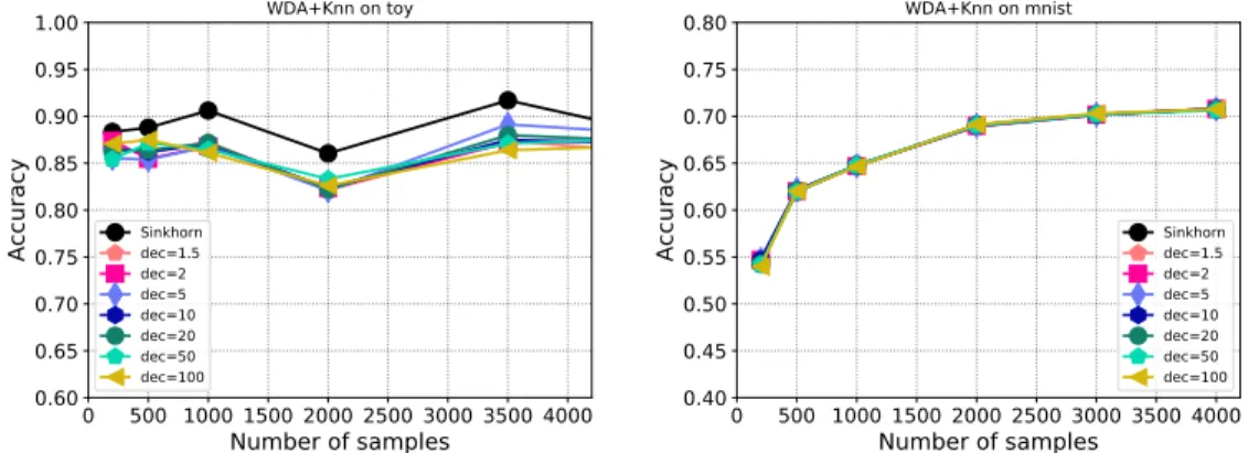
WDA+Knn on mnist Sinkhorn dec=1.5 dec=2 dec=5 dec=10 dec=20 dec=50 dec=100Figure 6: Accuracy of a1-nearest-neighbour after WDA for the (left) toy problem and, (right) MNIST). We note a slight loss of performance for the toy problem, whereas for MNIST, all approaches yield the same performance.
0 1000 2000 3000 4000 5000 Number of samples 0.6 0.7 0.8 0.9 1.0 1.1 1.2 Accuracy
Screened WDA+Knn on toy
Sinkhorn dec=1.5 dec=2 dec=5 dec=10 dec=20 dec=50 dec=100 0 1000 2000 3000 4000 5000 Number of samples 5 10 15 20 25
Running Time Gain
Screened WDA on toy
dec=1.5 dec=2 dec=5 dec=10 dec=20 dec=50 dec=100 0 1000 2000 3000 4000 5000 Number of samples 0.6 0.7 0.8 0.9 1.0 1.1 1.2 Accuracy
Screened WDA+Knn on toy
Sinkhorn dec=1.5 dec=2 dec=5 dec=10 dec=20 dec=50 dec=100 0 1000 2000 3000 4000 5000 Number of samples 2 4 6 8 10 12 14 16
Running Time Gain
Screened WDA on toy
dec=1.5 dec=2 dec=5 dec=10 dec=20 dec=50 dec=100
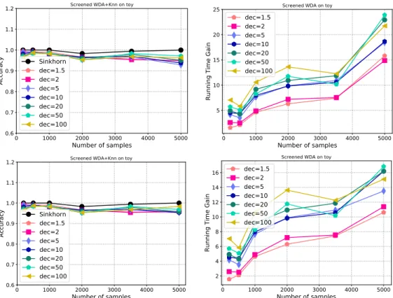
Figure 7: (top-left) Accuracy and (bottom-right) computational time gain on the toy dataset for
η = 0.1and1-nearest-neighbour. (bottom) accuracy and gain but for a5-nearest-neighbour. We can note that a slight loss of performances occur for larger training set sizes especially for1 -nearest-neighbour. Computational gains increase with the dataset size and are on average of the order of magnitude.
4 2 0 2 4 6 4 3 2 1 0 1 2 3 4 source 1 source 2 source 3 target 1 target 2 target 3 0 1000 2000 3000 4000 5000 Number of samples 0.4 0.5 0.6 0.7 0.8 0.9 1.0 Accuracy OTDA+Knn on toy Sinkhorn dec=1.5 dec=2 dec=5 dec=10 dec=20 dec=50 dec=100 No Adapt 0 1000 2000 3000 4000 5000 Number of samples 101 100 101 102 Running Time (s)
Screened OTDA on toy
Sinkhorn dec=1.5 dec=2 dec=5 dec=10 dec=20 dec=50 dec=100 0 1000 2000 3000 4000 5000 Number of samples 0 2 4 6 8 10
Running Time Gain
Screened OTDA on toy
dec=1.5 dec=2 dec=5 dec=10 dec=20 dec=50 dec=100
Figure 8: OT Domain Adaptation on a 3-class Gaussian toy problem. (top-left) Examples of source and target samples. (top-right) Evolution of the accuracy of a 1-nearest-neighbour classifier with respect to the number of samples. (bottom-left) Running time of the SINKHORNand SCREENKHORN for different decimation factors. (bottom-right). Gain in computation time. This toy problem is a problem in which classes are overlapping and distance between samples are rather limited. According to our analysis, this may be a situation in which SCREENKHORNmay result in smaller computational gain. We can remark that with respect to the accuracy SCREENKHORNwith decimation factors up to 10are competitive with SINKHORN, although a slight loss of performance. Regarding computational time, for this example, small decimation factors does not result in gain. However for above5-factor decimation, the gain goes from2to10depending on the number of samples.
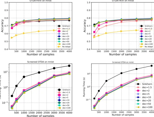
500 1000 1500 2000 2500 3000 3500 4000 Number of samples 0.4 0.5 0.6 0.7 0.8 0.9 1.0 Accuracy OTDA+Knn on mnist Sinkhorn dec=1.5 dec=2 dec=5 dec=10 dec=20 dec=50 dec=100 No Adapt 500 1000 1500 2000 2500 3000 3500 4000 Number of samples 0.4 0.5 0.6 0.7 0.8 0.9 1.0 Accuracy OTDA+Knn on mnist Sinkhorn dec=1.5 dec=2 dec=5 dec=10 dec=20 dec=50 dec=100 No Adapt 500 1000 1500 2000 2500 3000 3500 4000 Number of samples 101 100 101 Running Time (s)
Screened OTDA on mnist
Sinkhorn dec=1.5 dec=2 dec=5 dec=10 dec=20 dec=50 dec=100 500 1000 1500 2000 2500 3000 3500 4000 Number of samples 101 100 101 Running Time (s)
Screened OTDA on mnist
Sinkhorn dec=1.5 dec=2 dec=5 dec=10 dec=20 dec=50 dec=100
Figure 9: OT Domain adaptation MNIST to USPS : (top) Accuracy and (bottom) running time of SINKHORN and SCREENKHORN for hyperparameter of the`p,1 regularizer (left) λ = 1and
(right)λ= 10. Note that this value impacts the ground cost of each Sinkhorn problem involved in the iterative algorithm. The accuracy panels also report the performance of a1-NN when no-adaptation is performed. We remark that the strenght of the class-based regularization has influence on the performance of SCREENKHORN given a decimation factor. For small value on the left, SCREENKHORNslightly performs better than SINKHORN, while for large value, some decimation factors leads to loss of performances. Regarding, running time, we can note that SINKHORNis far less efficient than SCREENKHORNwith an order of magnitude for intermediate number of samples.
500 1000 1500 2000 2500 3000 3500 4000
Number of samples
0.4 0.5 0.6 0.7 0.8 0.9 1.0Accuracy
OTDA+Knn on mnist Sinkhorn dec=1.5 dec=2 dec=5 dec=10 dec=20 dec=50 dec=100 No Adapt 500 1000 1500 2000 2500 3000 3500 4000Number of samples
101 100 101 102Running Time (s)
Screened OTDA on mnist
Sinkhorn dec=1.5 dec=2 dec=5 dec=10 dec=20 dec=50 dec=100
Figure 10: OT Domain adaptation MNIST to USPS : (left) Accuracy and (right) running time of SINKHORNand SCREENKHORNfor the best performing (on average of10trials) hyperparameter`p,1
chosen among the set{0.1,1,5,10}. We can note that in this situation, there is not loss of accuracy while our SCREENKHORNis still about an order of magnitude more efficient than Sinkhorn.