University of South Florida
Scholar Commons
Graduate Theses and Dissertations
Graduate School
June 2018
Borromean: Preserving Binary Node Attribute
Distributions in Large Graph Generations
Clayton A. Gandy
University of South Florida, [email protected]
Follow this and additional works at:
https://scholarcommons.usf.edu/etd
Part of the
Computer Sciences Commons
This Thesis is brought to you for free and open access by the Graduate School at Scholar Commons. It has been accepted for inclusion in Graduate Theses and Dissertations by an authorized administrator of Scholar Commons. For more information, please [email protected].
Scholar Commons Citation
Gandy, Clayton A., "Borromean: Preserving Binary Node Attribute Distributions in Large Graph Generations" (2018).Graduate Theses and Dissertations.
Borromean: Preserving Binary Node Attribute Distributions in Large Graph Generations
by
Clayton A. Gandy
A thesis submitted in partial fulfillment of the requirements for the degree of Master of Science in Computer Science Department of Computer Science and Engineering
College of Engineering University of South Florida
Major Professor: Adriana Iamnitchi, Ph.D. Yicheng Tu, Ph.D.
John Skvoretz, Ph.D.
Date of Approval: June 11, 2018
Keywords: graph generators, social networks, dk graph models, binary node attribute networks Copyright © 2018, Clayton A. Gandy
DEDICATION
This work is dedicated to those whose perseverance helped bring it to fruition and to those I lost along the journey. My parents were invaluable for their support and steadfastness over the years. Thank you to my advisor Adriana Iamnitchi for teaching me how to be a storyteller.
ACKNOWLEDGMENTS
TABLE OF CONTENTS
LIST OF TABLES . . . iii
LIST OF FIGURES . . . v
ABSTRACT . . . vi
CHAPTER 1: INTRODUCTION . . . 1
1.1 Motivation . . . 1
1.2 DK-2 Graphs . . . 2
1.3 Objectives and Contributions . . . 5
CHAPTER 2: RELATED WORK . . . 7
2.1 Synthetic Graph Generation . . . 7
2.1.1 Kronecker Generation . . . 8
2.1.2 Block Two-Level Erdos-Renyi . . . 9
2.1.3 ERGMs . . . 9
2.1.4 Related DK Graph Generators . . . 10
2.1.4.1 DK 2.5 . . . 10
2.1.4.2 2K Simple . . . 10
2.2 Parallel Graph Processing Frameworks . . . 11
2.2.1 Giraph . . . 11
2.2.2 Darwini . . . 12
2.3 Graph Generators for Graph Anonymity . . . 13
2.3.1 Differential Privacy and DK-2 Graphs . . . 15
2.3.2 Pygmalion: Differentially Private DK-2 Graph Anonymization . . . 16
CHAPTER 3: DATASETS . . . 18
CHAPTER 4: ORBIS DK-2 TOPOLOGY GENERATOR . . . 20
4.1 dK Rewiring . . . 21
CHAPTER 5: BORROMEAN-SEQUENTIAL LABELED GRAPH GENERATION ALGORITHM . . 25
5.1 Comparison of Original Graphs vs. Borromean-S DK-2 Generations . . . 29
CHAPTER 6: BORROMEAN-PARALLEL LABELED GRAPH GENERATION ALGORITHM . . . 31
6.1 Stage 2: Partitioning the DK-2 Distribution . . . 32
6.2 Stage 4: Stitching the Subgraphs . . . 36
6.3 Performance of Borromean-P-Python . . . 42
CHAPTER 7: BORROMEAN-P SPARK: PARALLEL DESIGN AND IMPLEMENTATION . . . 52
7.1 Spark . . . 52
7.2 GraphX . . . 54
7.3 Tuning and Optimization . . . 55
7.4 Cluster Configuration . . . 55
7.5 Adapting the Parallel Merge Algorithm for Spark . . . 56
7.6 Performance of the Parallel Borromean . . . 57
CHAPTER 8: DISCUSSIONS AND FUTURE WORK . . . 60
8.1 Discussion of Results for All Algorithm Variants . . . 61
8.2 Future Work . . . 64
LIST OF TABLES
Table 3.1 Datasets Used in this Study . . . 19
Table 3.2 Labeled Attribute Percentages of the Datasets . . . 19
Table 4.1 Properties of Orbis-Generated DK-2 Unlabeled Graphs . . . 23
Table 5.1 Borromean-S Transitivity Comparison . . . 27
Table 5.2 Properties of Borromean-S Generated Labeled Graphs . . . 30
Table 5.3 Borromean-S Attribute Percentages . . . 30
Table 6.1 Sweden 5K Labeled 4-Partition Merge . . . 37
Table 6.2 Sweden 5K Four Partition Comparison . . . 38
Table 6.3 Sweden 5K Four Partition Comparison - Triads . . . 39
Table 6.4 Sweden 5K Ten Partition Comparison - Fractional and Kth. . . 40
Table 6.5 Sweden 5K Ten Partition Comparison - Fractional and Kth- Triads . . . 41
Table 6.6 Sweden 5K Ten Partition Comparison - Cross-Sectional and Random Shuffle . . . 42
Table 6.7 Sweden 5K Ten Partition Comparison - Cross-Sectional and Random Shuffle - Triads . . . . 43
Table 6.8 Sweden 50K Four Partition Comparison . . . 44
Table 6.9 Sweden 50K Four Partition Comparison - Triads . . . 45
Table 6.10 Sweden 50K Ten Partition Comparison - Cross-Sectional and Random Shuffle . . . 46
Table 6.11 Sweden 50K Ten Partition Comparison - Cross-Sectional and Random Shuffle - Triads . . 47
Table 6.12 Sweden 50K Ten Partition Comparison - Kth and Fractional . . . 48
Table 6.14 Properties of Labeled Graphs Generated with Borromean-P Python . . . 49
Table 6.15 Borromean-P Python Node Attribute Percentages . . . 50
Table 6.16 Borromean-P Python Performance (Time) . . . 50
Table 7.1 Properties of Borromean-P-Spark Graphs Generated in Parallel . . . 58
Table 7.2 Borromean-P-Spark Node Attribute Percentages . . . 59
Table 7.3 Borromean-P Spark - Parallel Performance (Time) . . . 59
Table 8.1 Label A Attribute Percentage Comparison . . . 61
Table 8.2 Label B Attribute Percentage Comparison . . . 61
Table 8.3 Edge Type A-A Percentage Comparison . . . 62
Table 8.4 Edge Type B-B Percentage Comparison . . . 62
Table 8.5 Edge Type A-B Percentage Comparison . . . 62
LIST OF FIGURES
Figure 1.1 The DK Series Representation of a Sample Graph . . . 3
Figure 1.2 Plot of the Degree Distribution of the Sweden Graph and Its Borromean-S Generation . . . 4
Figure 1.3 Plot of the Transitivity of the Sweden Graph and Its Borromean-S Generation . . . 4
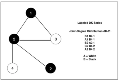
Figure 1.4 Labeled Sample Graph . . . 5
Figure 5.1 The Borromean-S (Labeled DK Series) Representation of a Sample Graph . . . 26
ABSTRACT
Real graph datasets are important for many science domains, from understanding epidemics to modeling traffic congestion. To facilitate access to realistic graph datasets, researchers proposed various graph gener-ators typically aimed at representing particular graph properties. While many such graph genergener-ators exist, there are few techniques for generating graphs where the nodes have binary attributes. Moreover, generating such graphs in which the distribution of the node attributes preserves real-world characteristics is still an open challenge.
This thesis introduces Borromean, a graph generating algorithm that creates synthetic graphs with binary node attributes in which the attributes obey an attribute-specific joint degree distribution. We show experi-mentally the accuracy of the generated graphs in terms of graph size, distribution of attributes, and distance from the original joint degree distribution. We also designed a parallel version of Borromean in order to generate larger graphs and show its performance.
Our experiments show that Borromean can generate graphs of hundreds of thousands of nodes in under 30 minutes, and these graphs preserve the distribution of binary node attributes within 40% on average.
CHAPTER 1: INTRODUCTION
Real social graph datasets are fundamental to understanding a variety of phenomena, such as epidemics, adoption of behavior, crowd management and political uprisings [1, 2, 3]. At the same time, many such datasets capturing these phenomena are often recorded now by individual researchers or by organizations. However, due to privacy concerns, many such datasets cannot be publicly shared. Moreover, for experi-mental investigations, there is always a need for more such datasets than are available. This work focuses on techniques for generating large graphs with binary node attributes and a specified joint-degree attribute-specific edge distribution.
1.1 Motivation
Many research problems and applications that involve graph datasets benefit from knowledge of specific node characteristics. Characteristic attributes of individual nodes may designate a state, condition, or affilia-tion that the node exhibits. Coupling these attributes with the tradiaffilia-tional node-edge relaaffilia-tionship informaaffilia-tion provided by graphs allows for the study of information flow and detailed analysis of node interaction.
A wealth of descriptive metadata may be available in the underlying data sets, but it is often useful to dis-till node characteristics into representative binary attributes, e.g. infected/non-infected, liberal/conservative, or student/teacher. Binary node attributes are important for the simulations of information dissemination scenarios, such as adoption of behavior or epidemic diffusion. Such labeling can also be used to predict the spread of other types of contagion [1].
Characterization of real data sets showed different particularities on such attributes. This work is mo-tivated by work done by Blackburn et al. [4, 5] that showed that node attribute values associate with node degree distribution and homophily. Specifically, users labeled as cheaters in the Steam Community online social network of gamers have a high level of homophily with other cheaters. That is, the more cheater
neighbors a player has, the more likely they are to be a cheater. Translated into graph metrics, the node attribute value is correlated with the number of edges connecting it with nodes with the same attribute value. While many graph generators exist, few focus on graphs with node attributes. The Erdos-Renyi [6] model generates unlabeled graphs connected with a given probability. Block Two-Level Erdos Renyi [7, 8] modifies the ER model through partitioning to generate graphs that conform to a given degree distribution and clustering coefficient.
The Barabasi-Albert [9] model generates graphs with power-law characteristics by means of preferential-attachment, such that new edges will be more likely to connect to already well-connected hub nodes. The Kronecker [10] model also generates power-law graphs, but through a recursive matrix product.
To enable attribute-aware applications, it is crucial to encapsulate the needed attribute information along with the node and edge structure in the graph representation. Graph generators have been proposed that incorporate node attributes. Skvoretz et al. [2] propose a model that assigns labels to nodes as a function of a homophily parameter. However, while it preserves in aggregate the concentration of edges connecting nodes with particular combinations of attributes, it does not conform precisely to the joint-degree distribution of the graph. In fact, each of these generators lacks a distribution of binary attributes to nodes that follows a particular joint-degree attribute-specific distribution.
1.2 DK-2 Graphs
An important family of graphs and their generators have been proposed by Mahadevan et al. in [11]. The dK series random graph model is based on graph feature extraction and random graph synthesis. The dK series is a graduated extraction of the degree distribution of connected components of sizeKwithin a graph.
dK(G):Gn→dx,dy;k (1.1)
Equation 1.1 is the formal function for the dK series, whereGis the input graph to be transformed [12]. n is the number of nodes in the graph. d is the degree of the respective connected components, andk is the number of connected components of sizeK={0,1,2,3}having that degree combination. Figure 1.1
illustrates the successive dK representations of a sample graph. In the dK-2 instance, the joint degree distributions of all two-node subgraphs are extracted. The dK-3 instance extracts the degrees of the three node triad distribution, which is helpful in accurately capturing the number of triangles in a graph, an important property for many real social networks referred to as theclustering coefficientin network analysis.
Figure 1.1: The DK Series Representation of a Sample Graph
Graphs generated from the dk series closely match the degree-based properties of their original graphs. As mentioned above and shown in Figure 1.1, each successive level of the series retains more property information about the degree distribution of nodes and their connected neighbors.
The dk-2 level gives a sufficient representation of the degree distributions of its original counterpart, as illustrated in Figure 1.2, though not of the clustering coefficient, shown in Figure 1.3. To accurately represent the clustering coefficient, the dk-3 level would be needed, but it is computationally intractable for large graphs [11].
The primary generator for the dk-2 level is the configuration [13] or pseudo-graph model. The configura-tion model pre-assigns edge end stubs to nodes equal to their degree and connects the edge ends at random. This technique reproduces given degree distributions exactly, but can produce self-loops and multi-edges.
● ● ● ● ● ● ● ●● ●●●●●●●●●●●●●●●●●●●●●●●●●●●●●●●● ●●●●●● ● ●●●●●●●●●●●●● ●● ●●●●●●●●●●●●● ●●●●●●●●●●●●●●●●● ●●●●●●●●●●●●●●●●●●●●● ● ●●●● ● ● ●●●●●● ●●●●● ● ●●●● ● ● ●● ● ●●● ● ● ●●● ● ●● ● ● ● ● ● ● ● ●● ● ● ●● ●●●● ●● ● ● ● ● ● ● ● ● ● ● ● ●●● ● ●●● ● ● ●●● ● ● ●● ● ● ●●● ● ● ● ● ● ● ● ● ● ● ● ●●●●●● ● ● ● ● ● ● ● ● ● ● ● ● ● ● ● ● ●● ● ● ● ●● 16 512 16384 524288 0 100 200 300 Node Degree Frequency (log)
● dK−2 graph original graph
Figure 1.2: Plot of the Degree Distribution of the Sweden Graph and Its Borromean-S Generation. The graph is a subset of the Steam gaming community player friendship graph consisting of Swedish players.
●● ●●●●●●●●● ●●● ●● ● ●●● ● ●● ●● ●●● ● ●●● ●●●● ● ●●●● ●●● ● ● ● ● ●●● ● ●● ●●●●●● ● ● ●● ● ●●●●●●● ● ●●●● ●●● ●● ● ● ●●●●●● ● ● ●●●● ● ● ● ●● ●●● ● ● ●● ● ● ● ●●● ● ●●●●● ●● ● ● ●●●● ●● ● ● ● ● ● ● ● ● ●●● ●● ● ●●●● ● ●●●●● ●● ● ● ● ● ● ● ●● ●● ● ● ● ●● ● ● ● ● ●● ● ● ● ● ● ● ●● ● ● ● ●● ● ● ● ● ● ●● ●● ●● ●●● ●● ● ● ● ● ● ● ●● ● ● ●●● ● ● ●● ●● ●● ● ● ● ●● ● ● ● ● ● ●● ● ● ● ● 2e−04 0.0039 0.0625 0 50 100 150 200 250 Node Degree Cluster
ing Coefficient (log)
● dK−2 graph original graph
Figure 1.3: Plot of the Transitivity of the Sweden Graph and Its Borromean-S Generation. The graph is a subset of the Steam gaming community player friendship graph consisting of Swedish players. Transitivity is the global clustering coefficient.
Mahadevan et al. [11] modify the configuration model to respect dk-2 joint-degree distributions and disallow self-loops and multi-edges.
The graph generation technique used in this work is based on the dk-2 level of the series and modifi-cations to the configuration model. We choose dk-2 for our work because of the prospect of developing a reasonable implementation and because it affords the opportunity to retain and study relationships between nodes.
1.3 Objectives and Contributions
The objectives of this thesis are twofold:
First, we want to generate labeled graphs with binary node attributes that follow a specific attribute-based joint-degree distribution. For example, let us assume we want to generate a graph in which a black node of degree 4 is connected with 2 black nodes of degrees 1 and 2 and 2 white nodes of degrees 1 and 2, as in Figure 1.4. In this case, white and black are the node binary attributes whose distribution we are interested in generating.
Figure 1.4: Labeled Sample Graph
Second, we want to be able to generate large graphs (in the order of hundreds of thousands nodes). The contributions of this thesis are:
1. We propose an algorithm, Borromean, for generating graphs with node attributes by modifying the dK-2 model. We are motivated to use dK-2 because it provides fidelity to the degree-based properties of the original graph. We implemented Borromean in C++ and refer to this sequential implementation as Borromean-S. We provide thorough experimental evaluations on six datasets from real networks. 2. We propose a parallel version of the algorithm to be able to generate larger graphs in reasonable time.
There are two key ideas in the design of the parallel version: the partitioning of the problem and the termination condition. The latter is meant to more accurately reproduce a desired average path length. 3. We propose the parallel algorithm in two versions. For testing the accuracy of the results we de-signed and implemented the parallel algorithm for Python. We refer to this version as Borromean-P-Python. For testing its performance in terms of execution time and scalability, we also designed and implemented the parallel Borromean algorithm for Apache Spark. We refer to this version as Borromean-P-Spark.
4. We also provide experimental evaluations on six datasets from real networks with binary node at-tributes.
The rest of the thesis is organized as follows:
• Chapter 2 provides the context for this work.
• Chapter 3 introduces the real datasets used for experiments. They are introduced early to allow us to describe experimental results related to particular topics addressed in subsequent chapters.
• Chapter 4 describes the dk-2 generation utility suite Orbis.
• Chapter 5 introduces our proposed sequential algorithm, Borromean-S, that is based on dk-2 models and generates node attribute-specific joint-degree distribution obeying graphs.
• In Chapter 6 we introduce and evaluate a parallel version of this algorithm that we name Borromean-P. • Chapter 7 describes and evaluates the parallel implementation in Spark [14] of Borromean-P.
CHAPTER 2: RELATED WORK
Significant effort has been invested into collecting, purchasing, or publishing social data for research. For example, Kwak et al. [15] collected the entire Twitter network as of 2010: 41.7 million user profiles, 1.47 billion social relations, 4.262 trending topics, and 106 million tweets. The Federal Energy Regulatory Commission published a repository of approximately 500,000 email messages of Enron Corporation, which has been frequently analyzed for research [16, 17]. AOL [18], Netflix, and Flickr [19] have all publicly released samples of their user graphs as part of crowd-sourced data-mining experiments.
These periodic releases do not provide sufficient data to model and simulate all possible structural char-acteristics and information flow needed to adequately address the multitude of research problems that require data. Researchers have turned in part to synthetic graph generation to fill the gap and provide more flexibil-ity. We discuss synthetic generation models in Section 2.1, with particular focus on generating dK graphs in Section 2.1.4.
The fact that the real graph data sets released were sampled and anonymized and still proved to be vul-nerable to re-identification from various modes of attack poses a privacy risk to users. We discuss anonymity models and their effects on the dk series in Section 2.3.
Graph data sets in the billions of nodes are so large that they cannot reasonably be processed by sequential methods. Algorithms are needed that allow them to be efficiently analyzed in parallel when distributed across a cluster of worker servers. We discuss parallel generation models in section 2.2.
2.1 Synthetic Graph Generation
Several models have been developed to allow these real world data sets to be synthetically mapped in graph relationships between nodes (i.e., users, emails, tweets, pages, locations, etc.). The synthetic models
attempt to capture various structural properties that can then be speculatively manipulated to service a myriad of hypothetical situations without compromising the original data.
Ultimately, graph generation is a question of intent and tuning of parameters. As previously stated, no synthetic generator can perfectly reproduce an original graph. Each has strengths and weaknesses with regard to individual properties, so a model must be chosen based on research interest.
For a simple example, the Erdos-Renyi [6] model generates graphs where nodes are connected with some probabilityp. Such random construction cannot capture degree distribution or clustering coefficient making it of little use structurally. Yet, many models augment ER with additional conditions, thereby generating graphs relatively closer to the degree distribution and clustering. Other models generate scale-free graphs where edge formation is not random but tends to concentrate from specific nodes. The most relevant of these models are described below.
Barabasi-Albert [9] generates graphs with power-law characteristics through probabilistic preferential-attachment. New edges have a higher probability to connect to nodes with greater degree. It does not respect fixed degree or attribute distributions.
2.1.1 Kronecker Generation
Lescovec et al. [10, 20] propose a means to mathematically model graphs with power-law characteris-tics through the recursive Kronecker product. The Kronecker product is the matrix direct product of two adjacency matrices, in this case, the product of the graph with itself.
In the resulting Kronecker graph, the original graph appears as interconnected sub-graphs up toktimes in the larger matrix. Stochastic Kronecker graphs form the edges of the adjacency matrix with a probability, p, in order to produce more continuous property distributions.
For standard power-law graphs, the Kronecker model captures degree and eigenvalue distribution, as well as densification, the gradual shortening of effective diameter as the graph grows. However, like Barabasi-Albert the Kronecker model does not accurately conform to graphs that do not follow power-law behavior, even for social networks with a fixed maximum degree.
The Kronecker model is related to work with densification in the forest fire model [21]. Forest Fire joins new nodes to the graph using a random breadth first search of existing edges, adding a one node then its neighbors, continuing recursively through the graph.
2.1.2 Block Two-Level Erdos-Renyi
BTER [7, 8] extends the Erdos-Renyi model to capture degree distribution and clustering coefficient through partitioning.d+1 nodes of degreedare grouped into community partitions. The community mem-bers are connected with a probability based on their maximum degree to form triangles approximating the local clustering coefficient. The communities are interconnected at random by edges between the remaining degree stubs in each community.
The BTER model is more flexible than the Kronecker in its ability to produce varying degree distributions departing from the power-law, but it cannot model dissociative graphs or graphs where the local clustering coefficient varies among nodes of the same degree.
2.1.3 ERGMs
Exponential random graph generation models are a family of probability distributions originally pro-posed to model directed graphs [22, 23]. ERGMs can regressively generate both directed and undirected graphs with a range of network properties from given distribution values such as degree or triangle count. While ERGMs can reproduce assortativity values, they cannot accurately reproduce joint degree distribu-tions.
Each network property can correspond to a space of possible graphs. The aim of ERGMs is to be able to generate as much of this space as statistically feasible. However, some portions of any space are not realizable, either because they do not produce stable graphs or because they would be the result of linear dependencies between properties.
2.1.4 Related DK Graph Generators
The dk graph model naturally preserves degree distributions and properties dependent thereupon, but does not preserve clustering related properties. Additionally, pseudo-graph matching generation loses edges that should be in the distribution due to the saturation of nodes with required degrees. The algorithms described in this section attempt to solve for these deficiencies.
2.1.4.1 DK 2.5
Gjoka et al. [24] propose the dk-2.5 model which improves the utility of dk-2 by specifically targeting the average clustering coefficient of the original graph. In the dk-2.5 algorithm, the joint degree distribution and clustering coefficient are estimated through a random walk of a sample of the original graph.
This process over-estimates lower degree nodes that are not easily surveyed by a random walk. The algorithm attempts to correct this using gaussian kernel smoothing; however, smoothing introduces floating-point values for degrees that must be rounded to integers and numbers of edges that cannot be matched given the existing nodes.
The algorithm uses a stochastic process (Markov Chain Monte Carlo sampling) during its swapping phase where it adds or deletes certain combinations of edges in order to minimize the error. The paper claims that this affects 3% of edges. However, MCMC is time consuming and may not converge at the targeted clustering coefficient [25].
2.1.4.2 2K Simple
2k_Simple [25] attempts to modify the Mahadevan et al. dk-2 compatible configuration model [26] in order to generate dk-2 graphs that exactly match the joint-degree distribution of the input graph. The most notable contribution of the work is a proposed solution to the edge starvation problem induced by earlier configuration approach. If a edge saturated vertex is encountered, the NeighborSwap function in moves an edge from the vertex with no open stubs to a vertex of equal potential degree and a free stub. The target node remains the same. Thus, the joint-degree distribution is completely preserved.
2K_Simple_Attributes extends 2K_Simple to add attribute awareness by matching source and target node degree along with their attributes to the joint-degree distribution. 2K_Simple_Attributes is the closest proposed alogrithm to Borromean in the literature. 2K_Simple_Clustering attempts to improve fidelity to the clustering coefficient by assigning nodes to a coordinate grid and connecting them by order of distance. The implementation used in 2K_Simple differs from Borromean-S, though both build from the config-uration model. 2K_Simple uses a custom graph class and NeighborSwap. The performance for 2K_Sim-ple_Attributes cannot be directly compared, as the source code for 2K_Sim2K_Sim-ple_Attributes and 2K_Simple_-Clustering has not been published.
2.2 Parallel Graph Processing Frameworks
2.2.1 Giraph
Apache Giraph is a graph analysis platform based on the vertex-centric bulk synchronous processing model similar to Pregel [27]. Facebook published a VLDB paper [28] describing the contributions they made to Giraph such that it could handle their production workloads of up to a trillion nodes. They also published a comparison [29] of the modified version of Giraph with Apache Spark’s GraphX library. Spark was originally designed to be the successor to Giraph.
Chiefly, the contributions of the paper improved memory overhead by storing worker data as byte arrays rather that Java objects, improved parallelism by instituting multi-threading per worker and a sharded aggre-gation model where random workers are chosen to gather the reduction results of their neighbors for global variables rather than bottleneck at a single central driver. The processing of incoming edge messages was also split so that multiple workers can process the traffic of a single well-connected vertex if needed.
Giraph performs the PageRank calculation 3 times faster than GraphX on a 1.5 billion edge sample of the Twitter graph with 16 workers, one per machine, and 80 GB of RAM. On a UK web graph with 3.7 billion edges, Giraph is 5 times faster. Giraph finds the connected components of the Twitter graph 5 times faster than GraphX. Giraph is also 3 times faster on average when calculating PageRank on a synthetic graph of 2 billion edges and 6 times faster finding connected components.
GraphX can complete PageRank on a 10 billion edge in approximately 18 minutes, and connected com-ponents in 12. Giraph is 4 and 8 times faster, respectively.
GraphX is limited in instances above 10 billion edges by high memory usage. Even with 2 billion edges, GraphX requires at least 20 GB per worker over sixteen machines.
The performance for triangle counts was also compared. Giraph completed the count in 40 minutes with 32 workers on the UK graph, but GraphX could not complete a count for a graph over 2 billion edges.
With 50 workers, page rank calculation using Giraph on a graph of 200 billion edges takes approximately 6 minutes. The page rank calculation exhibits a linear time increase as edges are added with a fixed number of workers. The horizontal scalability curve approaches 2 minutes when 300 workers are added. A page rank calculation over 1 trillion edges and 1.39 billion nodes was achieved in 3 minutes using 200 machines. While the modified Giraph shows better performance with basic graph analysis using the Pregel/BSP algorithms it is designed for, it is still not well-suited for graph transformations such as those we were able to perform in GraphX/Spark and are needed for Borromean. In Borromean, the graph must be deconstructed, manipulated, and remade. Spark is a wider, general purpose platform that allows greater customization and manipulation of data.
2.2.2 Darwini
Darwini [30] is a synthetic graph generator similar to BTER that runs on top of Giraph. Darwini marks each node with its target degree and target clustering coefficient before partitioning into communities. The algorithm groups vertices that participate in the same number of triangles into community partitions. Com-munities are connected, not at completely at random as in BTER, but according to the target distributions. The triangles are completed by adding edges according to the Erdos-Renyi model with a probability de-rived from the the clustering. After this stage, the vertices in each community are still under-connected. The degree distribution is completed by connecting random vertices between partitions. Communities can be formed with vertices having a heterogeneous number of triangles participated in. This may result in an incorrect clustering coefficient. The paper claims this is preferable to incomplete partitions. Thus, the
gen-erated degree and clustering coefficients are closer to the original than BTER, but the gengen-erated effective diameter cannot be controlled [31].
The algorithm uses these communities as a basis for parallelism. It processes each community in a parallel, distributed manner using the vertex-centric bulk synchronous parallel approach in GraphInc, giving linear scalability. Very large graphs are split into super-communities that span the highest density of nodes in a region. Processing proceeds within super-communities, then between, recursively. The algorithm is particularly memory intensive in instances where entire super-communities must be loaded, even though the graph as a whole need not be loaded. The algorithm can accommodate graph data sets with trillions of edges. The entire Facebook graph was processed in 7 hours on an industrial cluster.
2.3 Graph Generators for Graph Anonymity
As more property information, and therefore utility for research, is retained in synthetic models, the space of random graphs that can be generated while fitting the model is increasingly restrained. The generated graph will closely resemble the original input graph if all the structural information required to faithfully represent every property is retained.
However, researchers working with social graphs need to exercise particular sensitivity when publishing their data sets as they may contain a wealth of user identifiable information in both their nodes and struc-ture [32]. To this end, many graph generation models at least partially predicate their motivation on the need to privatize data, but anonymization methods such ask-anonymization [33], partitioning [34], differ-ential privacy [35], which we discuss in the next section, and dk-2 anonymized graph generation [11, 12] all retain some degree of vulnerability to deanonymization attacks [32, 36], particularly those aided by machine-learning [19].
K-anonymization [33] algorithms attempt to increase the size and homogeneity of candidate sets through various permutations such as addition, deletion or randomization of edges. A natural complication to re-identification are regions of the graph that are structurally isomorphic. When analyzing isomorphic regions, the attacker’s finest level of discernment is a candidate set that contains all isomorphic nodes. The attacker’s counter potential lies in his or her ability to refine the candidate set.K-anonymization ensures each member
node within a possible candidate set is homogeneous in terms of degree such that a node would be isometric tok−1 neighbors. Therefore, although not targeted to social network data publishing,k-anonymity protec-tion ensures that the informaprotec-tion for each person contained in a released data cannot be distinguished from at leastk−1 other individuals in the data [37].
Partition or class based anonymization algorithms [34] partition the graph according to similarity of structural features. Interaction between these partitions is limited and any inter-connection edges are consol-idated. The partitions in this way form candidate sets difficult for attackers to distinguish. Partitioning also provides anonymity by clustering nodes and edges into groups that are then represented in the anonymized graph as super-nodes [38].
While preserving user privacy, the published graph must also maintain as much utility as possible for structural analysis and research. Yet, the process of anonymization often distorts structural properties of rel-evance to researchers along with node identity. For example, existingk-anonymous graph models degrade the utility of degree-based metrics and in addition have prohibitive run times for large data sets. Even statis-tical generation models like differential privacy can obscure the utility of graph properties that are especially resistant to edge manipulation with the injection of copious noise. Thus, there is no comprehensive solution that provides unassailable privacy and utility while allowing unfettered distribution.
In many cases, data sets are released in anidentity-scrapedform, where personally identifying informa-tion associated with each user is either removed altogether or substituted with a random ID [39]. Yet sharing real social graphs, even with node-identifiable information removed, has been proven over and over again to be dangerous for the privacy of the individuals represented by the nodes of such graphs because naive anonymization does not in itself alter or obscure the structure of the graph. .
For example, in 2006 AOL released an anonymized data set of twenty million search keywords for over 650,000 users [40]. Despite the fact that the data released was identity-scraped, users’ privacy was compromised. To make the point, the New York Times identified an individual from this data set by cross referencing users with phone book listings [18].
In other cases, Narayanan et al. [19, 36, 41] demonstrated the feasibility of a large-scale machine-learn-ing based de-anonymization attack under the assumption that the attacker has background knowledge of a
different network whose membership partially overlaps with the target network. Machine-learning attacks bolster the attacker’s knowledge by training with this existing data. This training generates a vast array of background information which can be compared to potential target nodes. If the attacker has even partial knowledge of the adjacent edges to the target node, then it may well be possible to re-identify the target and its neighbors. The external information risk is high because basic identifying data is often public. Narayanan et al. showed that a third of the common users of Flickr and Twitter can be recognized in the completely anonymous Twitter graph with only 12% error rate.
Also, structural anonymization compromises the utility of the original graph. Aggarwal et al. [42] demonstrated that utility degrades very quickly while privacy is achieved very slowly in real, social net-works with approaches that randomly rewire the graph, due to hidden structural signatures in large, sparse networks.
2.3.1 Differential Privacy and DK-2 Graphs
Differential privacy is an anonymization method that injects statistical noise into a data set such that any one user will be indistinguishable from any other. Differential privacy algorithms [43, 35, 44] perturb the entries of a data set, e.g. the rows of a table or the edges of the graph, with probabilistic random noise such that the data of any given entry matches any other within a certain small limit,ε.
The perturbation attempts to address the problem of preserving the attributes and properties of a data set as a whole, in the original formulation a statistical database, while maintaining the anonymity of individual users. This technique is adapted in later literature [12, 45] to anonymize graphs as well. In each graph, structural properties have specific sensitivities to perturbation. The lower the sensitivity, the greater the noise required for anonymization of that property for the graph.
It is useful to understand how dk-2 graphs are affected by the differential privacy model. Sala et al. [12] apply the anonymization techniques of the model to dk-2 graphs. The dk-2 series is used as a non-interactive structural property query on graph data sets. The query extraction is executed, then the anonymization occurs once for the entire set as opposed to the interactive model where selected parts of the data are dynamically
anonymized as they are requested. Multiple dK models can be generated from the same data set without losing privacy.
The goal of the differential privacy condition is to produce an anonymized graph that is probabilistically close to the original graph within a factorε. Since the dK series extraction is the query in this instance, the probability of the output graph having the same structures as the original input graph should be within
ε. ε is inversely proportional to data fidelity; as ε grows, the similarity between the two graphs decreases.
Assume the neighbors ofGare similar graphs each differing by an edge. The sensitivity of the dK-2 series is the maximum number of changes in the set among neighbors. The sensitivity of dK-2,SdK−2, is bounded
by the maximum degree,dmax, specifically 4dmax+1.
In order to ensure anonymity with this method, the probability distributions of statistical property queries on both the original database and its counterpart must be statistically close. To meet the indistinguishability condition, the absolute value of the natural log of the ratio of the two distributions must be less than or equal to a small constant. In practice, the noise needed by differentially private anonymization is much too large to ensure accurate utility. Also, differentially private graphs are still vulnerable to machine-learning attacks.
2.3.2 Pygmalion: Differentially Private DK-2 Graph Anonymization
Sala et al.[12] propose Pygmalion, a differentially private graph model emphasizing edge privacy that statistically extracts the structure of the original graph as a degree correlation set using the dK-2 series model [11], then partitions this set using a degree-based clustering algorithm in order to minimize the noise needed to reach the differentially private condition.
The algorithm reduces the degree variance in each cluster. It is claimed that this reduction lessens the noise needed by an order of magnitude. The calculated noise is then injected into the set. Isotonic regression is used to evenly distribute the noise, mitigating the effective error, it is claimed, by 50%. Further, it is claimed that the generated graph is a close match to the standard metrics and experimental utility of the original graph.
Sala et al. use the Laplace mechanism to generate random noise. Unfortunately, the noise grows poly-nomially with node degree, so before noise is injected the dK-2 series set needs to be sorted and clustered. The expected noise error is far too large to produce graphs with any accuracy.
CHAPTER 3: DATASETS
We chose six publicly available datasets from four different contexts and generated networks with binary node attributes. The datasets include selections from the Facebook 100 university network collection labeled by faculty/student status [46], a political blogging network labeled by liberal/conservative affiliation [47], and a portion of the Amazon product network labeled by book/music product type [48]. The following details these data sets.
• polblogs[47] is an interaction network between political blogs during the lead up to the 2004 US presidential election. This dataset includes ground-truth labels identifying each blog as either conser-vative or liberal.
• fb-dartmouth, fb-michigan, andfb-caltech[46] are Facebook social networks extant at three US universities in 2005. A number of node attributes such as dorm, gender, graduation year, and academic major are available. We chose the occupation node attribute occupation, represented by the values “student” and “faculty”.
• amazon-products [48] is a bi-modal projection of categories in an Amazon product co-purchase network. Nodes are labeled as “book” or “music”, edges signify that the two items were purchased together.
• steam sweden [49] is a subset of the Steam online gaming service player friendship graph. The subset corresponds to the Swedish population of players.
Table 3.1: Datasets Used in this Study. Column Trans presents the clustering coefficient of the graph, and column Avg Path presents the average path length. Column Trans is the transitivity, or global clustering coefficient.
Data Set #Nodes # Edges Trans Avg Path Polblogs 1224 16718 0.22 2.49 FB-Caltech 769 16656 0.29 1.33 FB-Dartmouth 7694 304076 0.15 2.76 FB-Michigan 30147 1176516 0.13 3.05 Amazon Products 303551 835326 0.21 17.42 Steam Sweden 749878 2008476 0.13 6.10
Table 3.2: Labeled Attribute Percentages of the Datasets. Column A-A presents the percentage of edges that connect nodes of type A, B-B presents the percentage of edges that connect nodes of type B, and A-B the percentage of edges that connect nodes of different types.
Dataset Label A % Label B % A-A % B-B % A-B %
Polblogs 48 52 44 48 8 FB-Caltech 72 28 69 8 23 FB-Dartmouth 62 37 58 18 24 FB-Michigan 78 22 72 9 19 Amazon Products 81 18 83 2 16 Steam Sweden 97 2 84 0.9 14
CHAPTER 4: ORBIS DK-2 TOPOLOGY GENERATOR
The Orbis graph topology suite [11, 50] is a collection of utilities designed to generate and manipulate the dK series and its respective random, synthetic graphs. Orbis is written in C++ and requires the Boost graph library [51]. Graphs are represented by Boost AdjacencyList graph data structures, and the degree distributions are represented by nested map data structures from the C++ standard template library.
Orbis uses dK degree distributions to produce graphs exhibiting properties conforming to dK levels 0, 1, 2, and 3. Orbis can only directly generate dK-0, dK-1, dK-2 graphs. It uses edge rewiring algorithms to approximate dk-3.
In the dk-2 instance, the distribution list is of the form[du,dv,t], whereduis the degree of the first vertex in the pair,dvis the degree of the second vertex in the pair, andtis the total number of edge occurrences of pairs with those degrees in the graph. There is only one line per unique degree pair.
The dkDist utility extracts the dk degree distribution from the original graph. The algorithm for dkDist is shown as Listing 4.1.
Orbis’ primary means of dK-2 generation is a pseudo-graph matching, or configuration, algorithm im-plemented in dkTopoGen2k. The algorithm for dkTopoGen2k is shown as Listing 4.2.
dkTopoGen2k labels each node with edge ends in accordance with its degree. The ends match each edge in the edge set. The edge ends are randomly connected with the connect stubs procedure listed as Algorithm 4.3.
The edge stubs are connected with restrictions following the degree distribution of the original graph or the joint degree distribution in the dK-2 instance. For example, if the tuple in the JDD is(d,d0) =m, then an edge end corresponding to a node of degreedmust be connected to a target end on a node of degreed0. The
process will be repeated formedges and in turn for all tuples in the JDD. Edge ends will not be connected if it would result in a self-loop to the same node or a multi-edge with an extant edge between two nodes.
4.1 dK Rewiring
dK preserving rewiring is a random graph generation technique that moves edges between random pairs of nodes so long as such a move would preserve the properties of the given dK distribution. No edges are added or removed. For example, dK-2 rewiring must preserve the joint degree distribution and dK-3 rewiring must preserve wedge and triad distributions. Section 4.1.4 of [11] discusses the general approaches.
Movement of edges in this manner continues until the graph converges on a stable state where further rewirings do not alter dK distribution properties. The basic preserving algorithm requires the original graph and cannot create a random graph from a dK tuple list alone. It has a runtime ofO(m).
dK targeted rewiring moves from a dK graph to a higher, more descriptive level based on a target (tuple list) distribution. For example, a dK-2 graph can be rewired to a dK-3 graph based on a dK-3 tuple list. The algorithm is essentially a version of the Metropolis-Hastings algorithm, using Metropolis dynamics as an acceptance function.
Some graphs representing higher order dK levels are nonergodic, i.e. they do not converge to a desired stable state. This is chiefly exhibited in graphs having dK-4 or higher.
4.2 Limitations of the Orbis DK-2 Pseudo-Graph Generation Model
In combination with randomization, the degree matching, self-loop, and multi-edge restrictions of the pseudo-graph generation model can cause an edge starvation condition. The condition occurs because all eligible target edge ends have already been occupied before all edges in the JDD are formed. For example, the dk-2 graphs of each of the network samples of the Sweden subgraph differ in edge set cardinality from their original counterparts by approximately 1.1% fewer edges.
The pseudo-graph matching method becomes computationally impractical for dk-3 and above [12]. There is currently no graph generator algorithm forK greater than or equal to 3, as each level of fidelity
demands higher computation and storage requirements. This difficulty is concerning because social net-work research requires the preservation of community structures and metrics including the relationship of nodes with specific attributes to their neighbors. The dk-2 distribution shows this in part, but to study how cheating behavior propagates through the graph, it is also useful to measure the global clustering coeffi-cient, or transitivity, as shown in Equation 4.1. The dk-2 random graph generation model preserves degree-based properties but obscures clustering-degree-based properties. For example, we have empirically confirmed that the dK-2 distribution does not accurately preserve clustering coefficients. Table 4.1 shows the structural properties including the transitivity of graphs generated by the original Orbis unlabeled dk-2 pseudo-graph matching algorithm.
C= (number o f triangles)∗3/(number o f 2 paths) (4.1)
Algorithm 4.1DK-2 Distribution Generation (dkDist)
1: Input Graph G
2: Output Joint Degree Distribution
3: procedureREADINPUTGRAPH(Edge List)
4: foredge∈E do
5: set node degree in Boost graph structure
6: end for
7: end procedure
8: procedureGET2K DISTRIBUTION
9: foredge∈Boost graphGdo
10: retrieve Boost degree count for each node
11: increment JDD map (NKKMap) count based on degree combination
12: end for
Algorithm 4.2DK-2 Graph Generation (dkTopoGen2k)
1: procedureREAD2K DISTRIBUTION
2: fortuple∈dK-2 distributiondo 3: recreate NKKMap
4: end for
5: end procedure
6: procedureDKTOPOGEN2K 7: forlevel in NKKMapdo
8: approximate node count per degree (degree distribution NKMap)
9: round(edges / degree + 0.5)
10: end for
11: fordegree of each node in NKMapdo 12: create edge end stub structure
13: create list of stubs ordered by node degree
14: end for
15: shuffle stub list
16: initialize vector matrix of available stubs (all available)
17: create working copy from NKKMap
18: create randomly shuffled list of all stubs
19: end procedure
Table 4.1: Properties of Orbis-Generated DK-2 Unlabeled Graphs. The APL column is the effective diame-ter of the graph.
Data Set (GCC) Nodes Edges Transitivity APL Polblogs 1219 16667 0.17 2.93 FB-Caltech 760 16615 0.16 2.76 FB-Dartmouth 7679 304033 0.03 2.90 FB-Michigan 30027 1174804 0.01 3.33 Amazon Products 291274 803831 0.0001 7.27 Steam Sweden 739817 1992747 0.0001 5.87
Algorithm 4.3DK-2 Graph Generation (dkTopoGen2k Connect Stubs)
1: procedureCONNECTSTUBS
2: while6randomStubIds.empty()do
3: stubId = randomStubIds.front()
4: randomStubIds.pop_front()
5: ifavailable[stubId]then
6: get2kRandomDegree(stub.edge_type, stub.degree, workingMap)
7: total edges from workingMap[source degree]
8: target edge = rand() mod total edges
9: increment through workingMap[source degree] until target edge
10: targetDegree = second degree of target edge tuple
11: targetList = DegreeStubListMap[targetDegree]
12: forstub∈targetListdo
13: ifedge type match && available[stub] && edge not connectedthen 14: add_edge to Boost graph
15: set stubs as not available
16: decrement edge in workingMap
17: end if
18: end for
19: end if
20: end while
CHAPTER 5: BORROMEAN-SEQUENTIAL LABELED GRAPH GENERATION ALGORITHM
We have developed an algorithm for the generation of labeled graphs, Borromean-Sequential, that pre-serves the node attribute typed edge relationships from an original labeled graph within its randomly synthe-sized counterpart. Borromean-S generates labeled dk-2 graphs by modifying the algorithms used by Orbis. We selected the dK-2 distribution [26] because it provides a reasonable compromise between computational cost and fidelity with regard to graph metrics. The relevant procedures of the labeled algorithm are listed as Algorithms 5.1, 5.2, 5.3, and 5.4.
The first phase is found in the Borromean-S version of thedkDistutility, whose unlabeled Orbis imple-mentation is discussed in Chapter 4. The Algorithm 5.1 reads the original graph, notes the node attribute for each node, and counts the degree for each node. It then creates a nested map data structure,
Labeled_-NKKMap, containing the unique edge types as keys. Edge type is a string signifying the combination of node
attributes possessed by the edge ends. Specifically, it could be A-A, B-B, or A-B if the binary attributes for the graph were A and B. The algorithm uses an additional mirrored B-A edge type to distinguish the node attribute of the first node in the pairing found in the graph. The nested map is indexed as a multi-dimensional array with indexesiandj. Indexiis the degree of the first node in the pairing; indexjis the degree of the second. The corresponding value to each set of indexes is the total number of edges present for each com-bination. The complete map represents the labeled dk-2 joint-degree distribution. Finally, the distribution is written to a file. Figure 5.1 presents an overview of the Borromean-S labeled dk series distributions.
The second phase takes the distribution map file as input to the Borromean-S version of thedkTopoGen2k utility. The Algorithm 5.2 reads the labeled dk-2 distribution file to recreate theLabeled_NKKMap data structure. As in Chapter 4, Algorithm 5.3 then approximates the node count per degree by summing the total number of edges in the distribution and dividing by each degree. The algorithm creates the nodes of this count and assigns each node a number of edge ends, or stubs, equal to its degree. Algorithm 5.4 matches
Figure 5.1: The Borromean-S (Labeled DK Series) Representation of a Sample Graph
edge ends at random according to the distribution map. Edge ends must match both the node attributes and the degrees of the distribution pairing. Specifically, if the distribution pairing line isA 3 B 5 10, then the first node must be of attribute type A with degree 3, and the second node must be of attribute type B with degree 5. The algorithm connects matching ends with edges. Edge end matching continues until all eligible ends have been connected.
The resulting ratios of edges connected between node attribute types are statistically similar to the orig-inal graph. As shown in Table 5.2, respecting labeled attributes adds additional restrictions and further exacerbates edge starvation problem seen in Chapter 4 in some cases where the program is prevented from creating multi-edges between nodes. Type and degree appropriate target edge ends are randomly selected; it may be that the only remaining type appropriate edge end is on a node to which the source node is already connected.
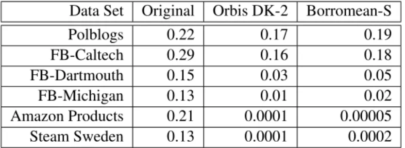
Theoretically, the additional restrictions on graph structure with regard to the labeling should improve the clustering coefficient. In general, our experiments show this to be true. Table 5.1 shows the clustering coefficient (transitivity) comparison for the original graph, the Orbis dk-2 generation, and the Borromean-S labeled generation. Borromean-S improves upon the transitivity versus Orbis in all data sets except for the Amazon products graph. The product co-purchase relationships do not represent a social network as the
other graphs do. The graph has relatively fewer edges for its node size, and the average path length is much greater.
Table 5.1: Borromean-S Transitivity Comparison. Clustering Coefficient (Transitivity) Comparison Be-tween the original graph, the Orbis dk-2 generation, and the Borromean-S generation.
Data Set Original Orbis DK-2 Borromean-S
Polblogs 0.22 0.17 0.19 FB-Caltech 0.29 0.16 0.18 FB-Dartmouth 0.15 0.03 0.05 FB-Michigan 0.13 0.01 0.02 Amazon Products 0.21 0.0001 0.00005 Steam Sweden 0.13 0.0001 0.0002
Our algorithm further restricts edge formation to nodes of specific labels or types based on attributes. In the Steam player friendship graph, VAC banned users are labeled cheaters (C) and non-VAC banned users are labeled non-cheaters (NC). The Steam graph as a whole as approximately 7% cheaters [49]. Thus, the graph has three types of edges: cheater to cheater (C-C), cheater to non-cheater (C-NC), and non-cheater to non-cheater (NC-NC). The algorithm uses four edge designations, adding the NC-C mirror of C-NC so as to distinguish mixed edge types and correctly identify the needed node attribute type of the target node.
Algorithm 5.1Borromean-S Labeled Distribution Generation (dkDist)
1: Input Graph G
2: Output Joint Degree Distribution
3: procedureREADINPUTGRAPH(Edge List)
4: foredge∈Edo
5: set node label and degree attributes in Boost graph structure
6: end for
7: end procedure
8: procedureGET2K DISTRIBUTION
9: foredge∈Boost graph Gdo
10: retrieve Boost degree count for each node
11: increment JDD map (labeled NKKMap) count based on degree combination and edge type
12: end for
Algorithm 5.2Borromean-S DK-2 Labeled (Read 2K Distribution)
1: procedureREAD2K DISTRIBUTION
2: fortuple∈labeled dK−2do
3: recreate labeled NKKMap
4: end for
5: end procedure
Algorithm 5.3Borromean-S DK-2 Labeled Graph Generation (dkTopoGen2k)
1: procedureDKTOPOGEN2K
2: forlevel∈labeled NKKMapdo
3: approximate node count per degree (degree distribution labeled NKMap)
4: round(edges/degree+0.5)
5: end for
6: fordegree of each node in labeled NKMapdo 7: create and label edge end stub structure
8: create list of stubs ordered by node label and degree
9: end for
10: shuffle stub list
11: initialize vector matrix of available stubs (all available)
12: create working copy from labeled NKKMap
13: create randomly shuffled list of all stubs
Algorithm 5.4Borromean-S DK-2 Labeled Graph Generation (Connect Stubs)
1: procedureCONNECTSTUBS
2: while6randomStubIds.empty()do
3: stubId = randomStubIds.front()
4: randomStubIds.pop_front()
5: ifavailable[stubId]then
6: get2kRandomDegree(stub.edge_type, stub.degree, workingMap)
7: total edges from workingMap[type][source degree]
8: target edge = rand() mod total edges
9: increment through workingMap[type][source degree] until target edge
10: targetDegree = second degree of target edge tuple
11: targetList = labeledDegreeStubListMap[label][targetDegree]
12: forstub∈targetListdo
13: ifedge type match && available[stub] && edge not connectedthen 14: add_edge to Boost graph
15: set stubs as not available
16: decrement edge in workingMap
17: end if
18: end for
19: end if
20: end while
21: end procedure
5.1 Comparison of Original Graphs vs. Borromean-S DK-2 Generations
In Table 5.2, we give the properties for the full Borromean-S labeled dk2 graphs generated from the data sets used. As described in Chapter 4, there is a loss of nodes and edges from the edge starvation of the pseudo-graph matching/configuration construction algorithm and the restriction of the graph to its greatest connected component. Such a restriction is reasonable since most social networks have a giant component that holds 50-90% of their nodes [52].
As expected, the accuracy of the clustering coefficient suffers greatly and the average path length is affected. The percentage of the second labeled attribute also drops, though the Facebook Dartmouth and Amazon product networks hold well.
Since dk-2 generation through psuedo-graph matching, and subsequently Borromean-S, damages the clustering coefficient, in the following iterations of the Borromean algorithm we specifically avoid breaking triangles.
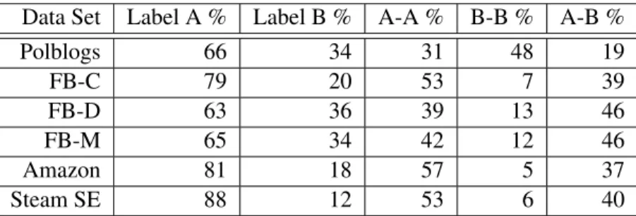
Table 5.3 presents the labeled attribute node and edge type percentages for the Borromean-S dk-2 gen-erated graphs. With the exception of the FB-Dartmouth and Amazon dk-2 graphs, there is a general loss of label A nodes and a gain in label B nodes. There is also a general loss of the label A-A edge type and a gain of the mixed label A-B edge type.
Table 5.2: Properties of Borromean-S Generated Labeled Graphs Data Set (GCC) Nodes Edges Transitivity APL
Polblogs 617 7839 0.19 2.77 FB-C 517 11508 0.18 2.48 FB-D 4076 176635 0.05 2.79 FB-M 20902 847570 0.02 2.97 Amazon 239515 673449 0.00005 6.92 Steam SE 643966 1681319 0.000185 5.97 (ED)
Table 5.3: Borromean-S Attribute Percentages
Data Set Label A % Label B % A-A % B-B % A-B %
Polblogs 66 34 31 48 19 FB-C 79 20 53 7 39 FB-D 63 36 39 13 46 FB-M 65 34 42 12 46 Amazon 81 18 57 5 37 Steam SE 88 12 53 6 40
CHAPTER 6: BORROMEAN-PARALLEL LABELED GRAPH GENERATION ALGORITHM
Borromean-S takes many hours to generate labeled dk-2 analogs for large graphs. Specifically, it takes more than 19 hours to generate a labeled dk-2 analog for the 750,000 node and 2 million edge Steam Sweden graph on a server with 32 GB of RAM. Since the generation and analysis of large graphs is a computationally intensive endeavor, we propose a parallel design and implementation for our labeled dk-2 synthetic random graph generation algorithm, Borromean-P. We chose Python for the initial implementation of Borromean-P because it is a highly extensible language with support for a large number of API modules providing graph transformation and analysis. Python is not a parallel language; however, we implement our algorithm in Python first to serve as a basis for further experiments in intrinsically parallel languages.
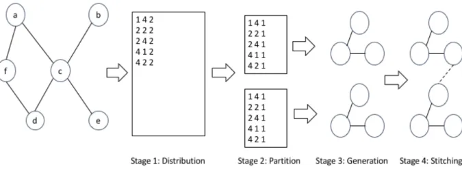
The four stages of the algorithmic design are illustrated in Figure 6.1 and described in detail below. The algorithm first extracts the dk-2 joint-degree distribution of an input graph using Borromean-S. The distribution is then subdivided into a given number of partitions. A dk-2 graph is generated from each partition using Borromean-S. Next the partition subgraphs are merged or stitched together by swapping edges between partitions. Edges with matching attribute types and degrees are identified in both subgraphs. The edges are swapped such that their terminal nodes are in different subgraphs. Specifically, an edge with an originating node of attribute A and degree 5 and a terminating node of attribute B and degree 7 in subgraph X is swapped with an edge of the same originating and terminating properties in subgraph Y. The originating node in subgraph X is connected to the terminating node in subgraph Y. Similarly, the originating node in subgraph Y is connected to the terminating node in subgraph X. The original connections are removed. In order to mitigate any further loss to the clustering of the graph, candidate edges for swapping must not be a part of existing triads. Swapping terminates when a given average path length is reached.
Figure 6.1: System Design Overview
In the first stage, the original graph is processed through the Borromean-S version of thedkDistutility to extract its signature as a listing of the joint degree distribution as detailed in Chapter 5. The procedure is illustrated in Stage 1 of Figure 6.1.
6.1 Stage 2: Partitioning the DK-2 Distribution
In the second stage of Borromean-P, we partition the dk-2 joint degree distribution before the any graphs are generated. It is useful to partition the graph generation into separate tasks to improve the tractability of our generation algorithm. The partitions provide a basis for parallel implementation allowing for faster processing on smaller portions of data and requiring less communication across workers. In addition, par-titioning provides access to a larger merged vertex set than does the un-partitioned GCC dk-2 generation. The dk-2 distribution is partitioned intoNsub-partitions of similar sizes.
We used 5,000 and 50,000 node samples of the Steam Sweden graph to test various methods of partition-ing the distribution. The graphs are sampled via breadth first search from randomly chosen cheater nodes
until the node size is reached and the percentage of cheater nodes reaches that of the original Steam Sweden graph.
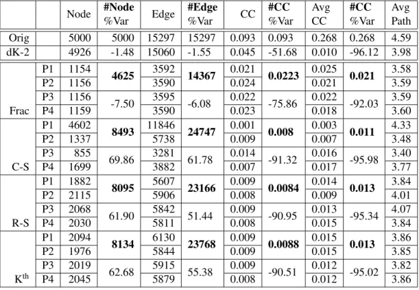
Tables 6.2, 6.4, 6.6, 6.8, 6.10, and 6.12 present our results in evaluating partitioning schemes. The tables also serve as a numerical comparison between the structural properties of the dk-2 graphs of the 5,000 and 50,000 node variations of the Sweden data set and their original analog. The relative differences between network properties are also quantified. We present results for four and ten partitions, respectively. The four schemes evaluated are cross-sectional, random shuffle, kth partition, and fractional. Our goal is to find a partitioning method that optimizes the balance of structural properties across partitions
Simple cross-sectional partitioning divides the dk-2 distribution across a given number of partitions. Random shuffle partitioning randomly sorts the listing, then divides the distribution as in cross-sectional. A Kth partitioning division moves distribution lines into partitions in a round robin fashion. The fractional method divides the total edges of each pair by the number of partitions N and distributes the integer ceiling of this edge quotient to each partition such that the distribution lines become[du,dv,dt/Ne].
In cross-sectional partitioning, the distribution is sorted in ascending order with larger total edge counts at the bottom of the listing resulting in the later partitions having a greatly imbalanced share of edges. Table 6.2 presents the nodes, edges, transitivity, average clustering coefficient, and average path length for the 4-way partitioning of the Sweden 5K Borromean-S labeled dk-2 graph. Cross-sectional partitioning results in one partition with 4602 nodes, one with 855, and an overall 69.86% increase from the original graph in nodes summed across partitions. The number of edges increases 61.78% overall. The transitivity drops 91.32%. Table 6.3 presents the triad properties for the Sweden 5K graph. The closed triads drop 93.23% from the original.
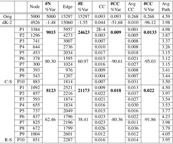
Table 6.6 presents the properties for the 10-way cross-sectional and random shuffle partitioning of the Sweden 5K graph. The nodes and edges are unevenly distributed as in the 4-way partitioning. One partition has 5957 edges while another has 976. The number of nodes increases 80.30%, and the number of edges increases 60.97%. The transitivity drops 90.61%, and the number of closed triads drops 90.75% as presented in Table 6.7.
Table 6.8 presents the properties for the 4-way partitioning of the Sweden 50K graph. The cross-sectional nodes and edges remain unevenly distributed with 48,488 nodes and 223,115 edges in partition subgraph 1. The number of nodes increases 46.65%, less than the 5K graph, but still significant. The number of edges increases 47.85%, and the transitivity decreases 89.35%, slightly less than the 5K. The closed triads decrease 88.15% as presented in Table 6.9. Table 6.10 presents the properties of the 10-way cross-sectional and random shuffle partitioning of the Sweden 50K graph. The cross-sectional nodes increase 73.20%, and the edges increase 68.60%. Partition subgraph 1 has 43,304 nodes and 151,489 edges. The transitivity decreases 89.70%, and the closed triads decrease 89.73% as presented in Table 6.11.
Random shuffle partitioning exhibits large total edge counts that may still imbalance the partitions con-sidering that distribution lines are placed in partitions with their whole count. The distribution of nodes in the random shuffle 4-way partitioning of the Sweden 5K graph is more even than the cross-sectional with the largest partition having 2115 nodes and the smallest having 1882. However, the total node count increases 61.90% from the original graph. The number of edges increases 51.44% overall. The transitivity drops 91.32%, and closed triads drop 90.14%.
In the random shuffle 10-way partitioning of the Sweden 5K graph, the largest partition has 1092 nodes and the smallest has 593. The number of nodes increases 62.46%, and the number of edges increases 38.41%. The transitivity drops 80.36%, and the number of closed triads drops 86.00%.
In the random shuffle 4-way partitioning of the Sweden 50K graph, the largest partition has 22,612 nodes, and the smallest has 19,980. The number of nodes increases 70.45%; the number of edges increases 66.42%. The transitivity decreases 93.43%, and the closed triads decrease 90.02%. In the random shuffle 10-way partitioning of the Sweden 50K graph, the nodes increase 83.87%, and the edges increase 74.18%. The largest partition has 10,291 nodes, and the smallest has 7,732. The transitivity decreases 87.60%, and the closed triads decrease 82.59% as presented in Table 6.11.
Kth partitioning suffers imbalances due to high total edge counts. The distribution of nodes in the Kth 4-way partitioning of the Sweden 5K graph is similar to the random shuffle with the largest partition having 2094 nodes and 6130 edges. The smallest partition has 1976 nodes and 5844 edges. The total node count
increases 62.68% from the original graph. The number of edges increases 55.38% overall. The transitivity drops 90.51%, and closed triads drop 89.18%.
Table 6.4 presents the properties for the Kthand fractional 10-way partitioning of the Sweden 5K graph. In the Kth10-way partitioning of the Sweden 5K graph, the largest partition has 926 nodes and the smallest has 618. The number of nodes increases 54.20%, and the number of edges increases 32.71%. The transitivity drops 82.21%, and the number of closed triads drops 87.95% as presented in Table 6.5.
In the Kth 4-way partitioning of the Sweden 50K graph, the largest partition has 22058 nodes, and the smallest has 21142. The number of nodes increases 73.05%; the number of edges increases 68.46%. The transitivity decreases 93.56%, and the closed triads decrease 90.03%. Table 6.12 presents the properties for the Kth and fractional 10-way partitioning of the Sweden 50K graph. In the Kth and fractional 10-way partitioning of the Sweden 50K graph, the nodes increase 83.11%, and the edges increase 73.61%. The largest partition has 9833 nodes, and the smallest has 8571. The transitivity decreases 88.11%, and the closed triads decrease 83.41% as presented in Table 6.13.
Fractional cross-sectioning yields the best balance for all properties across partitions and the best fidelity to the clustering coefficient of the original graph as a whole of the partitioning methods analyzed. The distribution of nodes in the fractional 4-way partitioning of the Sweden 5K graph is even with one partition having 1154 nodes, two having 1156, and one having 1159. The total node count decreases 7.50% from the original graph where the node count increases in the other methods. The distribution of edges is also even with two partitions having 3590, one having 3592, and one having 3595. The number of edges decreases 6.08% overall. The transitivity does drop 75.86%, but this is the lowest decrease of all the methods. The closed triads drop 85.67%.
In the fractional 10-way partitioning of the Sweden 5K graph, the partitions range in node set size from 530 to 537. The partition edge set sizes range from 1658 to 1678. The number of nodes increases 6.72%, and the number of edges increases 8.86%. The transitivity drops 42.25%, and the number of closed triads drops 66.61%.
In the fractional 4-way partitioning of the Sweden 50K graph, two partitions have 12474 nodes, one has 12494, and one has 12496. The partition edge sizes range from 66034 to 66110. The number of nodes
decreases 0.12%; the number of edges increases 3.34%. The transitivity decreases 83.05%, and the closed triads decrease 83.02%. In the fractional 10-way partitioning of the Sweden 50K graph, the nodes increase 6.97%, and the edges increase 20.41%. The partition node set sizes range from 5251 to 5358. The edge set sizes range from 30759 to 30816. The transitivity decreases 42.91%, and the closed triads decrease 27.07%. We choose the fractional method to partition the Borromean-S dk-2 distribution before any graphs are generated because it yields balanced partitions having relatively equal counts for both nodes and edges. In addition, it is the closest method to the original graph clustering coefficient overall.
In the third stage, dk-2 graphs are generated from the partitions using Borromean-S.
6.2 Stage 4: Stitching the Subgraphs
The final stage of the algorithm reconstitutes the full graph from the partitions. We take this opportunity to try to not to damage the transitivity and average path length of the resulting dk-2 graph further. The par-tition graphs are merged, or stitched, by swapping eligible edges across parpar-titions. Each parpar-tition maintains a list of its eligible edges. Eligible edges must:
• Maintain the dK-2 distribution
• Not disconnect connected components • Not be a part of an existing triad
Edges are swapped across partitions so long as the candidate for swapping is not in an existing triad and not a bridge between connected components. The objective is to preserve as much of the clustering and community structure as possible. Triads are identified by searching for common neighbors between two adjacent nodes. Bridge edges are detected by breath first search in a variant of Trajan’s bridge finding algorithm [53]. Table 6.1 presents the bridge, non-triad, and candidate edge counts for the 4-partition merge of the labeled Sweden 5K graph specifically.