Electrical and Computer Engineering Conference
Papers, Posters and Presentations
Electrical and Computer Engineering
11-2014
A Fast Proximal Gradient Algorithm for
Reconstructing Nonnegative Signals with Sparse
Transform Coefficients
Renliang Gu
Iowa State University, [email protected]
Aleksandar Dogandžić
Iowa State University, [email protected]
Follow this and additional works at:
http://lib.dr.iastate.edu/ece_conf
Part of the
Signal Processing Commons
This Conference Proceeding is brought to you for free and open access by the Electrical and Computer Engineering at Digital Repository @ Iowa State University. It has been accepted for inclusion in Electrical and Computer Engineering Conference Papers, Posters and Presentations by an authorized administrator of Digital Repository @ Iowa State University. For more information, please [email protected].
Recommended Citation
Gu, Renliang and Dogandžić, Aleksandar, "A Fast Proximal Gradient Algorithm for Reconstructing Nonnegative Signals with Sparse Transform Coefficients" (2014).Electrical and Computer Engineering Conference Papers, Posters and Presentations.Paper 4.
A Fast Proximal Gradient Algorithm for
Reconstructing Nonnegative Signals with Sparse
Transform Coefficients
Renliang Gu and Aleksandar Dogandˇzi´c
ECpE Department, Iowa State University, 3119 Coover Hall, Ames, IA 50011 email: frenliang,[email protected]
Abstract—We develop a fast proximal gradient scheme for reconstructing nonnegative signals that are sparse in a transform domain from underdetermined measurements. This signal model is motivated by tomographic applications where the signal of interest is known to be nonnegative because it represents a tissue or material density. We adopt the unconstrained regularization framework where the objective function to be minimized is a sum of a convex data fidelity (negative log-likelihood (NLL)) term and a regularization term that imposes signal nonnegativity and sparsity via an`1-norm constraint on the signal’s transform
coefficients. This objective function is minimized via Nesterov’s proximal-gradient method with function restart, where the prox-imal mapping is computed via alternating direction method of multipliers (ADMM). To accelerate the convergence, we develop an adaptive continuation scheme and a step-size selection scheme that accounts for varying local Lipschitz constant of the NLL. In the numerical examples, we consider Gaussian linear and Poisson generalized linear measurement models. We compare the proposed penalized NLL minimization approach and exist-ing signal reconstruction methods via compressed sensexist-ing and tomographic reconstruction experiments and demonstrate that, by exploiting both the nonnegativity of the underlying signal and sparsity of its wavelet coefficients, we can achieve significantly better reconstruction performance than the existing methods.
I . IN T R O D U C T I O N
Sparse signal reconstruction and compressed sensing [1] exploit the fact that most natural signals are well described by only a few significant coefficients in some [e.g., discrete wavelet transform (DWT)] domain, where the number of significant coefficients is much smaller than the signal size. Therefore, for anp1vectorxrepresenting the signal and an appropriate pp0 sparsifying transform matrix‰, we have
x D ‰s, where s is an p0 1 signal transform-coefficient
vector with most elements having negligible magnitudes. The idea behind compressed sensing is to sense the significant components of s using a small number of measurements (N < p): y D .x/ D .‰s/, where ./ W Rp 7! RN
represents the noiseless measurement vector model. For linear models, .x/D ˆx, where ˆ 2RNp is a known sensing matrix.
In [2], the signal transform coefficientsswere assumed to be
bothnonnegative and sparse in the same domain. In this paper, we consider nonnegative signalsxD‰swith sparse transform coefficientss, which is of significant practical interest and has immediate applications in tomography where the underlying This work was supported by the NSF under Grant CCF-1421480 and NSF I-U CRC Program, CNDE, Iowa State University.
image x represents a nonnegative quantity. Therefore, the nonnegative sparse signal model with the general sparsifying transform‰ ispractically more useful and challenging than that in [2]: It allows the signal of interest to be nonnegativeas well assparse in the appropriate transform domain. Harmanyet al. have recently considered such a nonnegative sparse signal model and developed in [3] and [4] a convex-relaxation sparse Poisson-intensity reconstruction algorithm (SPIRAL) and a linearly constrained gradient projection method for Poisson and Gaussian linear measurements, respectively; both schemes are part of the SPIRAL toolbox [5] and we label them SPIRAL in this paper. In [6], Qiu and Dogandˇzi´c developed an expectation-conditional maximization either (ECME) method for the linear measurement model with Gaussian noise, by adopting the difference-map iterations to find the minimum-distance pro-jections onto the intersection between the nonnegative and sparse signal constraint sets.
In this paper, we adopt the unconstrained regularization framework and minimize
f .x/DL.x/Cur.x/ (1a) with respect to the signal x, where L.x/ is a convex data fidelity term[negative log-likelihood (NLL)],u > 0is a scalar tuning constant, and
r.x/D k‰Txk1CIŒ0;C1/.x/ (1b)
is aregularization termthat imposes signal nonnegativity and sparsity.
We introduce the notation:kkp, “T”,0,1,I, denote the`p
norm, transpose, vectors of zeros and ones, and identity matrix, respectively. For a vectoraDŒa1; : : : ; aNT 2RN, define the
nonnegativity indicator function and projector
IŒ0;C1/.a/, ( 0; a0 C1; otherwise; .a/C i Dmax.ai; 0/
where “” is the elementwise version of “”; the el-ementwise logarithm lnı.a/ i D lnai and exponential expı.a/ i De
ai, and soft thresholding operator T.a/
iD
sign.ai/max jaij ; 0 .
I I . RE C O N S T R U C T I O N AL G O R I T H M
To minimize the objective function (1a), we employ the
Nesterov’s proximal-gradient (NPG) method [7, 8], whose ith
This is a manuscript of a proceeding in
Forty-Eighth Asilomar Conference on Signals, Systems and
Computers
(2014): 1-6. Posted with permission.
Iteration is .iC1/D 1 2 1C q 1C4 .i /2 (2a) x x.iC1/Dx.i /C .i / 1 .iC1/ x .i / x.i 1/ (2b) x.iC1/Dproxˇ.i /ur x x.iC1/ ˇ.i /rL xx.iC1/ (2c) whereˇ.i /> 0is the step size,rL.x/is the gradient of the
NLLL.x/with respect to the signalx, (2b) is the Nesterov’s acceleration step using the momentum, and (2c) is the proximal-gradient step. Here,
proxr.a/Darg min x
1
2kx ak 2
2Cr.x/ (3)
is the proximal operator for scaled (by > 0) regularization term (1b); the computation of (3) is discussed in Section II-A. We initialize (2) with x. 1/, choose .0/D 0 andx.0/ D
0 [9], and select the step size ˇ.i / to satisfy the following majorization condition: L.x.iC1//L.xx.iC1//C.x.iC1/ xx.iC1//TrL xx.iC1/ C 1 2ˇ.i /kx .iC1/ x x.iC1/k22: (4)
If L.x/is an L-smooth convex function, then
ˇ.i / 1
L (5)
guarantees that (4) holds, whereLis the Lipschitz constant of
L.x/. The proximal-gradient (PG) iterationwithoutNesterov’s acceleration [consisting of iterating only the PG step (2c)] is guaranteed to decrease monotonically the objective function (1a) when the majorization condition [(4) withxx.iC1/ replaced by x.i /] or (5) hold. The monotonic convergence conditions for the PG iteration do not carry over to the accelerated NPG iteration (2). To improve convergence of the NPG iteration, we restore its monotonicity by applying the “function restart” [10].
A. Proximal Mapping via (Linearized) ADMM
We now present a linearized alternating direction method of multipliers (ADMM) scheme [11, Sec. 4.4.2] for computing the proximal operator in (3):
z.jC1/D‰T ‰ T.˛.j / .j // (6a) ˛.jC1/D 1 1C aC z.jC1/C.j / C (6b) .jC1/D.j /Cz.jC1/ ˛.jC1/ (6c) where is a positive step size parameter, usually set to 1 [12, Sec. 11]. We obtain (6) by decomposing the proximal objective function (3) into the sum of 12k˛ ak22CIŒ0;C1/.˛/
and k‰T˛k1, and initialize it by ˛.0/ D .a/C and .0/ D
a .a/C. The iteration (6) is the exact ADMM algorithm when the dictionary matrix ‰ has orthonormal rows, i.e.,
‰‰T DI: (7)
B. Convergence Criteria
Define the convergence criterion of the outer iteration in (2) as the relative signal change between consecutive steps:
ı.i /, kx .i / x.i 1/ k2 kx.i /k 2 < (8a)
whereis the convergence threshold.
10−8 10−6 10−4 10−2 100 0 0.1 0.2 0.3 0.4 0.5 0.6 0.7 f ( x ) − f ⋆ CPU time/s FISTA (1/L) FISTA (BB) NPGS (adaptive)
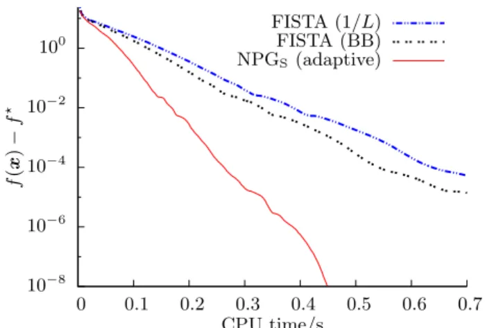
Figure 1: Centered objective function versus the CPU time for BPDN schemes with different step sizes and constant regularization parameteru.
1) Inner-iteration convergence criterion: Denote byi and
j are the outer and inner iteration indices corresponding to the NPG and ADMM iterations, respectively, and by˛.i;j /and z.i;j /the iterates of˛andzin thejth (inner) ADMM iteration step within the ith step of the (outer) NPG iteration (2). We set the following criterion for the inner ADMM iteration:
max ( kz.i;j / z.i;j 1/k2 kz.i;j /k 2 ;k˛ .i;j / ˛.i;j 1/k 2 k˛.i;j /k 2 ) < ıı.i 1/ (8b) where the convergence tuning constantı 2.0; 1/is chosen to trade the accuracy and speed of the inner iteration and provide sufficiently accurate PG steps (2c). Here,ı defines the level
of relative improvement in accuracy that inner ADMM loop needs to achieve compared with the outer loop’s convergence metricı.i 1/.
C. Adaptive Step Size Selection
Although the NLL functionL.x/may beL-smooth, the max-imal eigenvalue of its Hessian matrix may vary significantly with x [13]. Here, we propose a simple adaptive strategy to seek the largest step sizeˇ.i / that satisfies (4): in Iterationi,
if there has been no step size reductions fornconsecutive iterations, i.e.,ˇ.i 1/ D ˇ.i 2/ D D ˇ.i n 1/, start with a larger step size ˇ.i / D ˇ.iˇ1/, where ˇ 2 .0; 1/
is astep-size adaptation parameter; otherwise start with
ˇ.i /Dˇ.i 1/;
applybacktrackingwith multiplicative scaling constantˇ. This strategy keeps ˇ.i / as large as possible, subject to (4), especially when signal iterates reach a region where the local Lipschitz constant (within this region) ofL.x/is small.
Fig. 1 illustrates the advantage of adaptive step size com-pared with the constant inverse Lipschitz [see (5)] and Barzilai-Borwein (BB) (with backtracking) step sizes, see Section III-A for more details. Here, we impose signal sparsity only and consider basis pursuit denoising (BPDN). We employ an orthogonal sparsifying transform (DWT) matrix‰; hence, the two reconstruction methods NPGS(introduced in Section II-E)
and fast iterative shrinkage-thresholding algorithm (FISTA) in Fig. 1 are equivalent, except for the step size selection.
D. Adaptive Continuation
Continuation has been used in, e.g., [14, 15], to accelerate the convergence by decreasing the regularization parameter
u in (1a) from an initial value umax to the desired ufinal. The standard algorithm is called for eachuand the returned signal estimate is used to initialize the next round with a smaller u. This strategy stabilizes and effectively accelerates the convergence, especially for small regularization parameters, where the standard algorithms usually converges slowly.
Unlike existing continuation approaches [14, 15], we de-crease the convergence threshold at each uand denote the initial and final value ofbymax andfinal, withmaxfinal.
Define
U.x/,‰TrL.x/
1 (9a)
and note that U.0/is an upper bound on u; indeed, foruD
U.0/, minimizing (1a) yields the trivial optimum at x D 0. We select
umaxDminf ufinal; uU.0/g (9b) where1andu2.0; 1/are tuning constants that specify the range of values that the regularization parameter u can take in our continuation approach: is the largest possible ratio ofumax andufinal that we allow andu keepsumax from being too close to theU.0/. Reasonableumax is guaranteed by (9b) even for scenarios withU.0/D C1, e.g., Poisson model with identity link function [3]. In addition, the continuation is automatically disabled when ufinaluU.0/, becauseumax
ufinal.
We repeat the following steps untiluufinal:
keep running NPG (2) until convergence, with a decreas-ingconvergence threshold defined by
lnDlnfinalC
lnmax lnfinal lnumax lnufinal
.lnu lnufinal/ (10a) which maps Œlnmax;lnfinal linearly toŒlnumax;lnufinal.
when the intermediate threshold (10a) is met at Iterationi, set
u maxnmin˚uu; uU.x.i // ; ufinal o
(10b) where u 2 .0; 1/ guarantees the minimum rate of decrease ofu, thus ensuring thatudecreases sufficiently quickly.
Note that it is easy to prove thatu < U.x.i //is a sufficient condition for x.i / to not be optimal for the problem (1a) with
r.x/D k‰Txk1, which is why we ensure that this condition
holds when switching to the new uin (10b).
Here, our adaptive intermediate thresholds decrease to-gether with the regularization parameter u, thus reducing the possibility of premature convergence, which happens for constant large intermediate convergence thresholds (used, e.g., in [14]).
Our adaptation of u is general and allows optimization of (1a) for a wide range of differentiable NLLs L.x/. It is inspired by and generalized the continuation scheme in [14] for the Gaussian linear model. However, [14] does not
adapt the intermediate convergence thresholdand that, conse-quently, the sparse reconstruction by separable approximation (SpaRSA) method in [14] exhibits premature convergence in our numerical examples in Section III.
The minimum decrease rate constantuhelps in cases where
uU.x.i //does not go below ufinal, which can happen when the elements of rL.x.i // that correspond to zero elements in the estimate of x have large positive values, due to the nonnegativity constraints in (1b).
In summary, we introduce four tuning constants for our adaptive continuation, where andu control the initial value ofu,uandufurther control the descent ofu, and the initial intermediate thresholdmax decides the shift down ofufrom
umax. The performance of our methods is not sensitive to the selection of these parameters; we set their default values as
D104; uD10 2; uD0:5; maxD10 3 (11) that work generally well for most cases.
In the remainder of this paper (outside Section II-D), we simplify the terminology and refer toufinalandfinalasuand.
E. NPG for Signal Sparsity Only
We can apply our NPG method withr.x/D k‰Txk1 to
solve the`1-norm regularization problem: min
x L.x/Cuk‰
Tx
k1: (12)
Here, the proximal mapping has closed form, proxr.a/ D
‰T.‰Ta/, eliminating the need for the inner iteration. We label this algorithm as NPGS, where “S” emphasizes that this approach imposes signal sparsityonly. Similarly, we refer to the SpaRSA method in [14] for solving (12) as SpaRSAS.
I I I . NU M E R I C A L EX A M P L E
We now evaluate our proposed algorithm via numerical simulations. Relative square error (RSE) is adopted as the main metric to assess the performance of the compared algorithms:
RSED kyx xtruek
2 2
kxtruek22
(13) where xtrue and xy are the true and reconstructed signal, respectively.
All iterative methods use the convergence criterion (8a) with
D10 6 (14)
unless specified otherwise.
A. Linear Model and AWGN
Consider the linear measurement model with additive white Gaussian noise (AWGN), which leads to the NLL
L.x/D 1
2kˆx yk 2
2 (15)
where the elements of the sensing matrix ˆare independent, identically distributed (i.i.d.), drawn from the standard normal distribution. We have designed a “skyline” signal of length
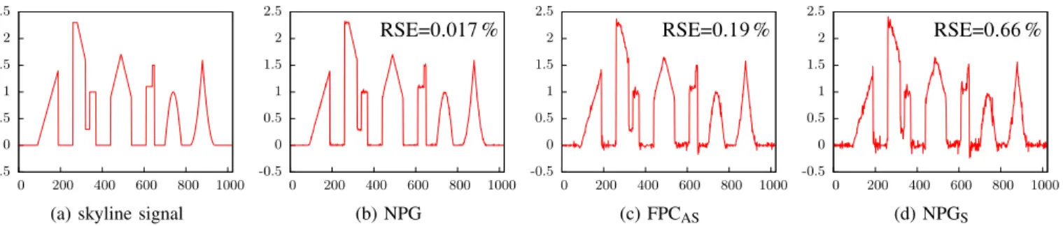
p D 1024 by overlapping magnified and shifted triangle, rectangle, sinusoid, and parabola functions, see Fig. 2a. The DWT matrix‰ is constructed using the Daubechies-4 wavelet with 3 decomposition levels, whose approximation by the 5% largest-magnitude wavelet coefficients achieves RSED98%. We consider the noiseless scenario with SNRD C1 and compare the following methods, grouped in two categories.
-0.5 0 0.5 1 1.5 2 2.5 0 200 400 600 800 1000
(a) skyline signal
-0.5 0 0.5 1 1.5 2 2.5 0 200 400 600 800 1000 RSE=0:017% (b) NPG -0.5 0 0.5 1 1.5 2 2.5 0 200 400 600 800 1000 RSE=0:19% (c) FPCAS -0.5 0 0.5 1 1.5 2 2.5 0 200 400 600 800 1000 RSE=0:66% (d) NPGS Figure 2: (a) The nonnegative ‘skyline’ signal and (b)–(c) its reconstructions forN=pD0:34.
(i) Nonnegative signal, sparse in DWT domain:
our NPG with convergence parameter ı D 10 3 and
adaptive continuation and step size parameters
nD4; ˇ D0:5 (16)
with Matlab implementation available at https://github. com/isucsp/npg,
SPIRAL for Gaussian linear model [4, 5], and
SpaRSA [14] with continuation and our implementation of the proximal mapping in Section II-A
all of which (aim to) solve the generalized analysis BPDN problem for nonnegative signals: minimize (1a) with NLL in (15) and regularization term in (1b).
(ii) Sparse signal in DWT domain:
Analysis:
– our NPGS algorithm with adaptive continuation and adaptive step size parametersnandˇ in (16),
– original SpaRSAS from [14]
which solve the standard analysis BPDN problem: mini-mize (12) with NLL in (15).
Synthesis:
– FISTA with function restart and BB step size,
– Glmnet [16, 17] with tuning constants selected so that it solves (17).
which solve the standard synthesis BPDN problem: min s 1 2ky ˆ‰sk 2 2Cuksk1 (17)
and obtain the signal estimate as xy D ‰s.C1/, where s.C1/ is the vector of the transform signal coefficients obtained upon convergence;
– fixed-point continuation active set (FPCAS) method [15] based on the synthesis BPDN problem (17). Since we employ the orthogonal DWT sparsifying dictionary matrix withp0Dp, (7) holds and, furthermore,
‰‰T D‰T‰DI (18)
which implies that the analysis and synthesis BPDN formu-lations are equivalent; hence, NPGS, SpaRSAS, FISTA, and Glmnet aim at solving the same optimization problem; FPCAS is closely related and can be thought of as providingdebiased
BPDN solutions. All methods have been initialized by the approximate minimum-norm estimate:
x.0/DˆT
E.ˆˆT/ 1yDˆTy: (19)
The regularization parameter uhas the following form:
uD10aU.0/
where ais an integer selected from the intervalΠ7; 1. The other tuning options for SPIRAL and FPCAS are kept to their default values.
Fig. 1 shows the centered objective function f .x/ f?
(f?Dmin
xf .x/) as a function of the CPU time for a random realization of the sensing matrix with N=p D 0:24 samples andaD 3. The methods shown do not employ continuation because we wish to isolate the effect of the step size. Note that this advantage of our adaptive step size is persistent among different random realizations of the sensing matrix.
Figs. 2b–2d present the NPG, FPCAS, and NPGS reconstruc-tions, respectively, for a random realization of the sensing matrix withN=pD0:34. Here, imposing signal nonnegativity improves greatly the overall reconstruction anddoes notsimply rectify the signal values close to zero. The RSE metrics of methods that impose signal sparsity only have been computed without truncation of the final signal estimate (to make it nonnegative). RSE improvement brought by such truncation is minor: Indeed, truncating the FPCASand NPGSreconstructions will reduce their RSEs from0:19% to0:16% and from0:63% to0:55%, respectively, in Fig. 2c. Since NPGS, FISTA, and Glmnet achieve almost identical RSE performances, we show only that of NPGS in Figs. 2 and 3.
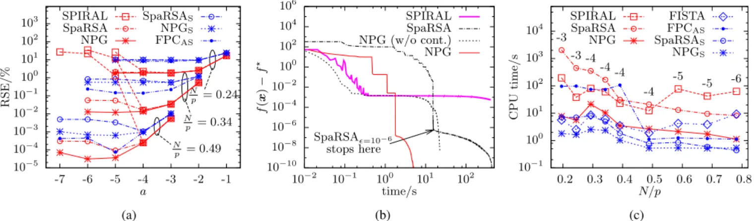
In Fig. 3a, we show the average RSEs (over 20 random realizations of the sensing matrix) as functions of the regular-ization parametera for normalized numbers of measurements
N=p 2 f0:24; 0:34; 0:49g. The methods from group (i) that impose both signal sparsity and nonnegativity are marked in red whereas the traditional methods from group (ii) that impose signal sparsityonly are marked in blue. For eachN=p, groups (i) and (ii) are well separated, with NPG achieving as much as 10 times smaller RSEs than FPCAS, the best among group (ii), thus showing the benefit of incorporating the prior information brought by the nonnegativity signal constraint. SPIRAL starts to fail asadecreases below 4: in this case, itdoes notreach the optimum of the objective function in (1a) and also yields reconstructions with much larger RSEs than NPG, see Fig. 3a. FPCAS performs the best within group (ii) because it inte-grates thedebiasing[18] into each iteration step via active set selection [15]. Indeed, the signal estimate provided by FPCAS also does not minimize (12) because of the debiasing. Note that our NPG and NPGS methods do not perform debiasing, though it is possible to implement it along the lines of [18].
10−5 10−4 10−3 10−2 10−1 100 101 102 103 -7 -6 -5 -4 -3 -2 -1 RSE/% a N p = 0.24 N p = 0.34 N p = 0.49 SPIRAL SpaRSA NPG SpaRSAS NPGS FPCAS (a) 10−10 10−8 10−6 10−4 10−2 100 102 104 106 10−2 10−1 100 101 102 f ( x ) − f ⋆ time/s SpaRSAϵ=10−6 stops here SPIRAL SpaRSA NPG (w/o cont.) NPG (b) 10−1 100 101 102 103 104 0.2 0.3 0.4 0.5 0.6 0.7 0.8 CPU time/s N/p SPIRAL SpaRSA NPG FISTA FPCAS SpaRSAS NPGS -3 -3 -4 -4 -4 -4 -5 -5 -6 (c)
Figure 3: (a) Average RSEs of different methods versus the regularization parameter a, (b) centered objective function versus the CPU time for different methods for one realization of the sensing matrix with N=pD0:49, and (c) average CPU times versus the normalized number of measurementsN=p with constanta2Π3; 6(labeled above) for eachN=p.
For N=p D 0:49, both SpaRSA and SpaRSAS converge prematurely, before reaching the optimum achieved by NPG and NPGS, respectively, for which a 5. We observe premature convergence of SpaRSA for N=p D 0:34 as well. Fig. 3b shows the centered objective function versus the CPU time for a random realization of the sensing matrix with
N=pD0:49andaD 6. Here, SpaRSA and SPIRAL are run beyond their convergence points mandated by (14), showing that SpaRSAdoesand SPIRALdoes notbenefit from running additional iterations. The premature convergence of SpaRSA is caused by its constant intermediate thresholds in continuation and the slow convergence rate afterwards is due to its first-order gradient descent algorithm. Note that the “knee” in the SpaRSA performance curve occurs at the place where its continuation is completed, i.e., the regularization parameterureachesufinal, see Section II-D. This phenomenon is observed in all 20 trials. To illustrate the benefits of continuation to the convergence of the NPG scheme, we show in Fig. 3b the NPG iterations with and without continuation.
As before, nonnegativity truncation of the signal estimates from group (ii) brings limited (up to 20%) improvement to the RSEs of these methods and does not change the general conclusions regarding their reconstruction performance.
Fig. 3c compares the CPU times of different methods as functions ofN=p. To be fair to SPIRAL, we use the smallest
a before SPIRAL starts to fail and list the values of a for eachN=p in the top part of Fig. 3c (shown as black-colored numbers). Our NPG method is at least 3 times faster than the methods from group (ii) that solve the same nonnegative and sparse signal reconstruction problem. Similarly, our NPGS performs the best overall within group (ii), but with limited advantage compared with the other methods. Hence, NPGS is competitive (in terms of computational speed) with the state-of-the-art approaches such as SpaRSASand FISTA. Its advantage compared with the closely related FISTA can be attributed to adaptive step size and continuation that NPGS employs. Note that FPCAShits occasionally the maximum-number-of-iteration limit (104), which explains its oscillatory behavior.
B. Application in X-ray CT Image Reconstruction
We now construct a simulated X-ray computed tomography (CT) example based on an10241024image, i.e., a collection of glass beads with different densities. The 2-D DWT matrix
‰ is constructed by the Daubechies-2 wavelet with level 4. The measurement matrixˆand its transposeˆT are the
fan-beam projection matrix and its adjoint operator, implemented on the GPU platform with circular mask [19]. The distance from X-ray source to the rotation center of the platform is
16 600times the image pixel size. Assuming the projections are equally spaced, we vary the number of projections from 60 to 360, which is equivalent to N=p 2 Œ3:7; 22:5. Each projection is collected by a detector array with 1024 elements.
We use theexponential attenuationmeasurement model [20, Sec. 4.1]:
E.y/D.x/DI0expı. ˆx/ (20)
where I0 is the unknown incident energy before
attenua-tion. (Models with unknown I0 have been used for disease
mapping in statistical epidemiology [21, Sec. 8.3.1].) Under the assumption of Poisson measurement y, we obtain the following concentrated NLL by replacingI0 in the NLL with
its maximum likelihood estimation as a function of x:
Lc.x/D1Tyln1Texpı. ˆx/CyTˆx: (21)
We compare the conventional filtered backprojection (FBP) [20] method and our NPG and NPGS methods that represent groups (i) and (ii). Note that FBP does not impose signal sparsity or nonnegativity.
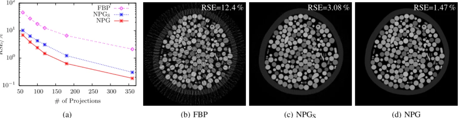
Fig. 4a shows the RSEs for different number of projections. The differences between FBP, NPGS and NPG suggests the benefit that sparsity and nonnegativity regularization could bring, respectively.
Finally, Fig. 4 shows the reconstructions and corresponding RSEs by the three algorithms from 120 projections. Here we show all the images in the same gray-scale range, starting from zero; hence, we effectively perform nonnegativity truncation in the FBP and NPGS reconstructions. It is clear that NPG reconstruction is visually the best, with smoother and better bead reconstructions. The RSEs listed in Fig. 4 are based
10−1 100 101 102 50 100 150 200 250 300 350 RSE/% # of Projections FBP NPGS NPG (a) RSE=12:4% (b) FBP RSE=3:08% (c) NPGS RSE=1:47% (d) NPG
Figure 4: (a) RSEs versus the number of projections and (a) FBP, (b) NPGSand (c) NPG reconstructions from 120 projections.
on the reconstructions without truncation. The corresponding truncated RSE are lowered to9:46% and2:83% for FBP and NPGS, respectively.
I V. CO N C L U S I O N
To solve our nonnegative sparse signal reconstruction prob-lem, we employed a proximal-gradient scheme with Nesterov’s acceleration and restart and proposed adaptive step size se-lection and continuation. We computed proximal mapping via linearized ADMM. Our NPG approach is computationally efficient compared with the state-of-the-art.
RE F E R E N C E S
[1] D. Donoho, “Compressed sensing”, IEEE Trans. Inf. Theory, vol. 52, no. 4, pp. 1289–1306, Apr. 2006. [2] D. L. Donoho and J. Tanner, “Sparse nonnegative
so-lution of underdetermined linear equations by linear programming”, Proc. Nat. Acad. Sci., vol. 102, no. 27, pp. 9446–9451, 2005.
[3] Z. T. Harmany, R. F. Marcia, and R. M. Willett, “This is SPIRAL-TAP: Sparse Poisson intensity reconstruction algorithms—theory and practice”, IEEE Trans. Image Process., vol. 21, no. 3, pp. 1084–1096, Mar. 2012. [4] Z. Harmany, D. Thompson, R. Willett, and R. F. Marcia,
“Gradient projection for linearly constrained convex optimization in sparse signal recovery”, in IEEE Int. Conf. Image Process., 2010, pp. 3361–3364.
[5] The sparse Poisson intensity reconstruction algorithms (SPIRAL) toolbox, accessed 27-November-2013. [On-line]. Available: http://drz.ac/code/spiraltap/SPIRALTAP. zip.
[6] K. Qiu and A. Dogandˇzi´c, “Nonnegative signal recon-struction from compressive samples via a difference map ECME algorithm”, inProc. IEEE Workshop Stat. Signal Process., Nice, France, Jun. 2011, pp. 561–564. [7] Y. Nesterov, “A method of solving a convex
program-ming problem with convergence rateO.1=k2/”, inSov. Math. Dokl., vol. 27, 1983, pp. 372–376.
[8] Y. Nesterov, “Gradient methods for minimizing com-posite functions”, Math. Program., vol. 140, no. 1, pp. 125–161, 2013.
[9] A. Beck and M. Teboulle, “A fast iterative shrinkage-thresholding algorithm for linear inverse problems”,
SIAM J. Imag. Sci., vol. 2, no. 1, pp. 183–202, 2009.
[10] B. O‘Donoghue and E. Cand`es, “Adaptive restart for accelerated gradient schemes”,Found. Comput. Math., pp. 1–18, Jul. 2013.
[11] N. Parikh and S. Boyd, “Proximal algorithms”,Found. Trends Optim., vol. 1, no. 3, pp. 123–231, 2013. [12] S. Boyd, N. Parikh, E. Chu, B. Peleato, and J. Eckstein,
“Distributed optimization and statistical learning via the alternating direction method of multipliers”,Found. Trends Machine Learning, vol. 3, no. 1, pp. 1–122, 2011. [13] Q. Tran-Dinh, A. Kyrillidis, and V. Cevher, “Composite
self-concordant minimization”, J. Mach. Learn. Res., 2014, in press.
[14] S. J. Wright, R. D. Nowak, and M. A. T. Figueiredo, “Sparse reconstruction by separable approximation”,
IEEE Trans. Signal Process., vol. 57, no. 7, pp. 2479– 2493, 2009.
[15] Z. Wen, W. Yin, D. Goldfarb, and Y. Zhang, “A fast algorithm for sparse reconstruction based on shrinkage, subspace optimization, and continuation”,SIAM J. Sci. Comput., vol. 32, no. 4, pp. 1832–1857, 2010.
[16] J. Friedman, T. Hastie, H. H¨ofling, and R. Tibshirani, “Pathwise coordinate optimization”,Ann. Appl. Stat., vol. 1, no. 2, pp. 302–332, 2007.
[17] J. Qian, T. Hastie, J. Friedman, R. Tibshirani, and N. Simon,Glmnet for Matlab, accessed 30-October-2014, 2013. [Online]. Available: http : / / www. stanford . edu /
hastie/glmnet matlab/.
[18] M. A. T. Figueiredo, R. D. Nowak, and S. J. Wright, “Gradient projection for sparse reconstruction: Applica-tion to compressed sensing and other inverse problems”,
IEEE J. Sel. Topics Signal Process., vol. 1, no. 4, pp. 586–597, 2007.
[19] A. Dogandˇzi´c, R. Gu, and K. Qiu, “Mask iterative hard thresholding algorithms for sparse image reconstruction of objects with known contour”, inProc. Asilomar Conf. Signals, Syst. Comput., Pacific Grove, CA, Nov. 2011, pp. 2111–2116.
[20] A. C. Kak and M. Slaney,Principles of Computerized Tomographic Imaging. New York: IEEE Press, 1988. [21] A. B. Lawson,Statistical Methods in Spatial