Coverage Problem
Irving van Heuven van Staereling
1, Bart de Keijzer
2, and
Guido Schäfer
31 Centrum Wiskunde & Informatica (CWI), Networks and Optimization Group, Amsterdam, The Netherlands
heuven@cwi.nl
2 Centrum Wiskunde & Informatica (CWI), Networks and Optimization Group, Amsterdam, The Netherlands
keijzer@cwi.nl
3 Centrum Wiskunde & Informatica (CWI), Networks and Optimization Group, Amsterdam, The Netherlands; and
Vrije Universiteit Amsterdam, Department of Econometrics and Operations Research, Amsterdam, The Netherlands
schaefer@cwi.nl
Abstract
We study the following natural variant of the budgeted maximum coverage problem: We are given a budgetBand a hypergraphG= (V, E), where each vertex has a non-negative cost and a non-negative profit. The goal is to select a set of hyperedgesT ⊆Esuch that the total cost of the vertices covered byTis at mostBand the total profit of all covered vertices is maximized. Besides being a natural generalization of the well-studied maximum coverage problem, our motivation for investigating this problem originates from its application in the context of bid optimization in sponsored search auctions, such as Google AdWords.
It is easily seen that this problem is strictly harder than budgeted max coverage, which means that the problem is (1−1/e)-inapproximable. The difference of our problem to the budgeted maximum coverage problem is that the costs are associated with the covered vertices instead of the selected hyperedges. As it turns out, this difference refutes the applicability of standard greedy approaches which are used to obtain constant factor approximation algorithms for several other variants of the maximum coverage problem. Our main results are as follows:
We obtain a (1−1/√e)/2-approximation algorithm for graphs.
We derive a fully polynomial-time approximation scheme (FPTAS) if the incidence graph of the hypergraph is a forest (i.e., the hypergraph isBerge-acyclic). We also extend this result to incidence graphs with a fixed-size feedback hyperedge node set.
We give a (1−ε)/(2d2)-approximation algorithm for everyε > 0, wheredis the maximum degree of a vertex in the hypergraph.
1998 ACM Subject Classification F.2.2 Nonnumerical Algorithms and Problems
Keywords and phrases maximum coverage problem, approximation algorithms, hypergraphs, submodular optimization, sponsored search
Digital Object Identifier 10.4230/LIPIcs.MFCS.2016.50
1
Introduction
In thebudgeted maximum coverage problem we are given a hypergraphG= (V, E) with a non-negative costc(e)∈R≥0for every hyperedgee∈Eand a non-negative profitp(i)∈R≥0
© Irving van Heuven van Staereling, Bart de Keijzer, and Guido Schäfer; licensed under Creative Commons License CC-BY
for every vertexi∈V, and a non-negative budget B∈R≥0. The goal is to select a set of
hyperedgesT ⊆E whose total cost is at mostB such that the total profit of all vertices covered by the hyperedges inT is maximized.
This is a fundamental combinatorial optimization problem with many applications in resource allocation, job scheduling and facility location (see, e.g., [6] for examples). Feige [4] showed that this problem is not polynomial-time approximable within a factor of (1−1/e) unlessNP⊆DTIME(nO(log logn)), even if all hyperedges have unit cost. Khuller, Moss and Naor [9] derived a (1−1/e)-approximation algorithm for the budgeted maximum coverage problem (which is the best possible). Their algorithms are based on a natural greedy approach in combination with a standard enumeration technique. Similar approaches were used to derive constant factor approximation algorithms for several other variants and generalizations of the maximum coverage problem.
In this paper, we study the following natural variant of the budgeted maximum coverage problem, which we call theground-set-cost budgeted maximum coverage problem (GBMC): We are given a hypergraph G = (V, E) with a non-negative cost c(i) ∈ R≥0 and a
non-negative profitp(i)∈R≥0for every vertexi∈V, and a non-negative budgetB∈R≥0. For a
subsetT ⊆E, definec(T) =P
i∈∪Tc(i) and p(T) =
P
i∈∪Tp(i) as the total cost and profit,
respectively, of all vertices covered by the hyperedges inT.1 Our goal is to select a set of
hyperedgesT ⊆E such that the total costc(T) of all covered vertices is at mostB and the total profitp(T) of all covered vertices is maximized. To the best of our knowledge, this problem has not been studied before.
Note that a crucial difference here is that in our problem costs are incurred per covered vertex, while in the budgeted maximum coverage problem costs are incurred per selected hyperedge. Albeit seemingly minor, this change makes the problem much harder to tackle algorithmically. More specifically, most greedy approaches (which give rise to constant factor approximation guarantees for several variants of the maximum coverage problem) turn out to be inapplicable in our setting because of the following reason: The basic idea underlying these greedy approaches is to select in each iteration a hyperedge that is mostcost-efficient, i.e., maximizes the ratio of the profit of newly covered vertices over the cost of selecting the hyperedge. A property that is crucially exploited in the analysis of these algorithms is that the cost for selecting a hyperedge is constant, i.e., its cost-efficiency can only decrease throughout the course of the algorithm (as more of its vertices get covered). However, this monotonicity property is no longer guaranteed in our setting because the cost for picking a hyperedge depends on the set of already covered vertices. In fact, it is not hard to see that the cost-efficiency of a hyperedge can change arbitrarily from one iteration to the next.
Our motivation for investigating the vertex-cost budgeted maximum coverage problem is two-fold: (i) It is a generalization of the well-studied maximum coverage problem and a natural variant of the budgeted maximum coverage problem. (ii) It is a fundamental combinatorial optimization problem having several applications in practice. Of particular importance is its relation to the problem of computing optimal bids in sponsored search auctions such as Google AdWords (details will be given in the full version of the paper).
Our contributions
The contributions presented in this paper are as follows:
1. We obtain a (1−1/√e)/2-approximation algorithm for graphs (Sections 2 and 3).
1 Throughout this paper, for a collection of setsF we write∪F to refer to the set∪ S∈FS.
The main idea here is to reduce this problem to the budgeted maximum coverage problem with an exponential number of hyperedges. However, we do not need to generate the exponentially large instance explicitly; but instead we make use of a concise representation of the instance and show that such instances can be approximated in polynomial time, given that we have access to an oracle that can select in polynomial time a hyperedge with approximately highest profit per unit of cost. As a last step in our reduction, we prove that such an oracle exists.
2. We derive in Section 5 a pseudo-polynomial time algorithm for the case when the incidence graph of the hypergraph is a forest (i.e., the hypergraph isBerge-acyclic). Further, we adapt this algorithm into a fully polynomial-time approximation scheme (FPTAS). At the core of this algorithm lies a bi-level dynamic program. The case of forests is important in its own right and, additionally, this algorithm constitutes an important building block of our O(1/d2)-approximation algorithm (see Contribution 4).
3. In Section 6, we extend the above algorithm to a pseudo-polynomial time algorithm for incidence graphs with a bounded set of nodes that covers all cycles (i.e., the general case, but parametrized).
More specifically, we show that for any incidence graph with a fixed-sizefeedback hyperedge node set, i.e., a hyperedge node set such that removing it from the incidence graph leaves no cycles, there exists a pseudo-polynomial time algorithm for the GBMC problem. 4. We give a (1−ε)/(2d2)-approximation algorithm for everyε >0 for the general case,
wheredis the maximum degree of a vertex in the hypergraph (Section 4).
In this algorithm, we first decompose the incidence graph of the hypergraph into a collection of at mostdtrees for which we compute an approximate solution by using our FPTAS for forests above. From this we then extract a solution that is feasible for the original instance and guarantees an approximation ratio of at least (1−ε)/(2d2).
Related work
Much literature is available on the maximum coverage problem and its variants (see, e.g., [1, 3, 9] and the references therein). Most related to our problem is the budgeted maximum coverage problem [9]. As outlined above, the greedy approach of [9] cannot take into account that the costs are incurred per vertex instead of per set. Moreover, in [3], a generalized version of the budgeted maximum coverage problem is studied, but this generalization does not include GBMC as a special case.
Note that our GBMC problem on graphs reduces to the knapsack problem if the incidence graph is a matching. This problem is known to be weaklyNP-hard and admits an FPTAS (see, e.g., [8]).
Our GBMC problem is related to thebudgeted bid optimization problem. This problem was first proposed in the paper by Feldman et al. [5]. The authors derive a (1− 1/e)-approximation algorithm if the budget constraint issoft, i.e., has to be met in expectation only. In contrast, in the budgeted bid optimization problem considered here, this budget constraint is hard.
The GBMC problem can be seen as a special case of a more general set of problems where we have to maximize a submodular profit function subject to the constraint that a submodular cost function does not exceed a given budget. This can be seen by considering the set of hyperedges to be the ground set of the submodular functions. However, when we have oracle access to both submodular functions, it has been shown that this more general problem is not approximable within a factor of log(m)/√m, where m is the number of elements in the ground set. This holds even for the special case that the objective function is
the modular function that returns the cardinality of the set. This follows from Theorem 4.2 in [10]; see also [7].
Preliminaries
For an integera∈N, we write [a] and [a]0 to denote the sets {1, . . . , a} and{0,1, . . . , a}
respectively. WhenF is a family of sets, we writeSF to denote the set S
S∈FS.
LetG= (V, E) be a hypergraph. Theincidence graphI(G) ofGis defined as the bipartite graphI(G) = (E∪V, H) withH ={{e, v} |v∈e}. We say thatGisacyclicif its incidence graphI(G) does not contain a cycle. Given a subsetE0⊆E, we useG[E0] to refer to the
subgraph of Ginduced by the hyperedges inE0, i.e., G[E0] = (V0, E0) with V0 =∪E0. A hypergraphT is called asubtree ofGifT is a subgraph ofGthat is acyclic.
Throughout this paper we will use the convention that when discussing a hypergraph,n denotes the number of vertices of the hypergraph andmdenotes the number of hyperedges of the hypergraph. Moreover, in the remainder of this paper, we assume without loss of generality that all costs (on the nodes or edges) are strictly positive.
It is not hard to prove that GBMC cannot be approximated to within a factor of (1−1/e) in polynomial time, unlessNP ⊆DTIME(nO(log logn)) (details will be provided in the full
version of the paper).
Due to space limitations, some figures and technical content is omitted from this paper and will be provided in the full version.
2
Budgeted Maximum Coverage with Oracles
In this section we first consider the classical budgeted maximum coverage problem. The result presented in this section will serve as a building block in the approximation algorithm presented in the next section, for solving GBMC on graphs.
A polynomial-time (1−1/e)-approximation algorithm for the budgeted maximum coverage problem was previously given in [9]. In the same paper, various simpler algorithms with worse approximation factors are presented. In this section, we present a variation of one of these algorithms that achieves a (1−1/e)/2-approximation guarantee, which can run even if the algorithm is not granted direct access to the input instance. We make this precise in the following definition.
IDefinition 1 (cost-efficiency oracle). Let I = (G= (V, E), c, p, B) be an instance of the budgeted maximum coverage problem, i.e., G= (V, E) is a hypergraph, c : E →Q≥0 is
a function that specifies a cost c(e) for each hyperedge e∈ E, p: V → Qis a function that specifies a profitp(i) for each vertexi ∈V, with B ∈ Qthe budget. For α∈[0,1], anα-approximate cost-efficiency oracle forI is a functionfI : 2V →Ethat maps a set of
verticesS⊆V to a hyperedgee∈E such thatc(e)≤B and X i∈e\S p(i) c(e) ≥α· X i∈e0\S p(i) c(e0).
for all e0 ∈ E withc(e0) ≤B. Thus, a cost-efficiency oracle takes as input vertex set S and selects the hyperedge with the approximately highest cost-efficiency (up to a factorα), excluding the profit that would be contributed by vertices inS. Only hyperedges of which the cost does not exceed the budget are considered.
LetI= (G= (V, E), c, p, B) be an instance of the budgeted maximum coverage problem, and letfI be anα-approximate cost-efficiency oracle for this instance for some α∈(0,1].
Consider now the following greedy algorithmAthat takes as input only the cost-efficiency oraclefI.
1. Set S := ∅andX := ∅. Throughout the execution of the algorithm, X represents a feasible solution and S represents the set of vertices covered byX.
2. Let e := fI(S). If S = V (i.e., there is no profitable hyperedge left) or if c(e) +
P
e0∈Xc(e0)> B (i.e., adding the hyperedge to X would exceed the budget), go to Step
3. Otherwise, set X:=X∪ {e}, set S=SX, and repeat this step.
3. Output the solution with the highest total profit among the two solutionsX and{e}.
I Theorem 2. Algorithm A outputs an (1−1/eα)/2-approximate solution to I in time
O(n·t), wheret is the amount of time it takes to evaluatefI.
The approximation factor is obtained by following rather closely the analysis given in [9] for a similar algorithm (that works without oracle access).
3
GBMC on Graphs
In this section, we present a (1−1/√e)/2-approximation algorithm for the GBMC problem when the hypergraph is a graph. We do this by reducing the problem to the budgeted maximum coverage problem. An instance I of GBMC is reduced to an instance r(I) of budgeted maximum coverage on the same set of vertices, such that the optimal solution of r(I) has the same profit as the optimal solution of I. The instance r(I) may have a superpolynomial number of hyperedges. However, instead of generating the budgeted maximum coverage instance explicitly, we construct only a 1/2-approximate cost-efficiency oraclefr(I)forr(I). We then use AlgorithmAonfr(I)in order to obtain a (1−1/
√
e)/2-approximately optimal solution tor(I) in polynomial time. Last, we show how to transform in polynomial time a feasible solution forr(I) into a feasible solution for Iwith equal profit.
We begin by defining our reduction r.
IDefinition 3. LetI= (G= (V, E), c, p, B) be an instance of GBMC whereGis a graph. Define the budgeted maximum coverage instancer(I) asr(I) = (G0= (V, E0), c0, p, B), where
E0 = [
i∈V
Ei0 and Ei0={S∪ {i} | ∀i0∈S:{i0, i} ∈E},
that is,Ei0 consists of the hyperedgesX such thatiis inX and all other vertices in X are connected toi by an edge. In other words,E0 are all hyperedges corresponding to the stars ofG. The cost functionc0 assigns a cost to eachhyperedge: for a hyperedgee∈E0 we set c0(e) =P
i∈ec(i). Note that c is a function that assigns a cost to eachvertex, whilec
0 is
a function that assigns a cost to each hyperedge in E0. Note that the vertex sets, profit functions, and budgets ofI andr(I) are equal.
We first show that every feasible solution X0 forr(I) can be transformed into a feasible solutionX forIin polynomial time such that the profit is preserved. Consider the following functiongI that maps solutions ofr(I) toI:
I Definition 4. Let I = (G= (V, E), c, p, B) be an instance of GBMC and let X0 be a feasible solution forr(I) = (G0 = (V, E0), c0, p, B). The functiongI mapsX0 to the following
solution forI. gI(X0) = n {i0, i} ∈E {i 0, i} ∈[ Xo.
ILemma 5. LetX0 be a feasible solution for r(I). The edge set gI(X0)is computable in
time O(mn|X0|). Moreover, the solutiongI(X0)is feasible (i.e., the total cost of all vertices
covered by gI(X0)does not exceedB). Also, p(X0) =p(gI(X0)).
Proof. For the first claim, observe that for each hyperedge inX0 and edge inE we need to check if that edge is contained in the hyperedge. This can be done inO(n) time.
The second claim follows from the fact that the edge setgI(X0) covers the same vertex
set asX0, and by definition B≥ X e∈X0 c0(e) = X i∈SX0 c(i)· |{e∈X0 :i∈e}| ≥ X i∈SX0 c(i) = X i∈SX0 c(i).
The third claim follows from the fact that the edge setgI(X0) covers the same vertex set
asX0. J
Next we show that the optimal solution forI is at most the profit of the optimal solution forr(I). (Combined with the previous lemma, this entails that the optimal profits ofI and r(I) are equal.)
ILemma 6. Letpoptbe the maximum profit achievable in instanceI. There exists a solution forr(I)with profitpopt.
Proof. LetXbe a profit-maximizing feasible solution forI. Assume without loss of generality that all paths inX are of size at most 2. In other words: no edge inX covers two vertices that are both covered by another edge (such an edge can be removed fromX without decreasing the profit). Under this assumption,X is a set of stars. We construct fromX a feasible solutionX0 forr(I) that has the same profit, as follows. We defineX0 to be the collection of hyperedges that correspond to the maximal stars ofX, i.e., for each maximal star ofX, we add toX0 the hyperedge consisting of the vertices covered by the star.
Since no pair of hyperedges inX0 intersects, by definition ofc0 the total costP
e∈X0c0(e)
equalsP
i∈SXc(i)< B, and thereforeX
0 is a feasible solution forr(I). Moreover,X0 and
X cover the same set of vertices, and therefore profits ofX inI equals the profit ofX0 in
r(I). J
A final ingredient that we need is a 1/2-approximate cost-efficiency oraclef forr(I).
IDefinition 7. We define the function f algorithmically as follows. Let S be the input argument tof. (As a reminder,S represents the set of vertices already covered during the execution of algorithmA.) The high level idea is that we compute for each vertexia set of verticesei in the star centered ati. Our goal for each of these stars is to select for each such
ithe substar with the (approximately) highest possible cost-efficiency, such that the cost of the vertices in the substar does not exceed the budget. We output the set in{ei:i∈V}
that has the highest cost-efficiency.
1. Let V0 be subset of vertices of V that have at least one neighbor not inS. For each i∈V0 (note thatiitself may be inS):
a.Initializeei:={i}, anddi=c(i). Ifi∈S, set ni:= 0, and otherwise setni:=p(i).
b.Order non-increasingly the verticesi0 that are not inS and are attached to iin graph
G, according to ratiop(i0)/c(i0). Denote this ordering byσi.
c.Leti0be the next vertex ofσi(starting with the first vertex). If (ni+p(i0))/(di+c(i0))≥
ni/di, then addi0toei, setni:=ni+p(i0), and setdi:=di+c(i0), and repeat this step in
case the total cost ofeidoes not exceedB. Otherwise, if (ni+p(i0))/(di+c(i0))< ni/di
d.If the total cost ofei lies within the budget, skip this step. Otherwise, leti0 be the
vertex last added in the previous step (i.e., the vertex in eiwith the leastp(i0)/c(i0)).
We consider two substars ofei that are within the budget: The one consisting only
of vertices iandi0, and the one consisting of vertices ei\ {i0}. We setei to be the
substar with the highest cost-efficiency. Formally:
i. Ifi6∈S: if (p(i) +p(i0))/(c(i) +c(i0))≥(ni−p(i0))/(di−p(i0)) then setei={i, i0},
ni:=p(i) +p(i0), anddi:=c(i) +c(i0). Otherwise setei:=ei\ {i0},ni :=ni−p(i0),
anddi:=di−c(i0).
ii. If i ∈ S: if p(i0)/(c(i) +c(i0)) ≥ (ni−p(i0))/(di −p(i0)) then set ei := {i, i0},
ni:=p(i0), anddi:=c(i) +c(i0) otherwise setei:=ei\ {i0}, ni :=ni−p(i0), and
di:=di−c(i0).
2. Output the set in{ei:|ei| ≥2∧i∈V0} with the highest cost-efficiency (i.e., the ratio
ni/di).
ILemma 8. The functionf is a1/2-approximate cost-efficiency oracle for r(I)and can be computed in timeO(n2).
Proof. It is easy to see that the set output by f is always a hyperedge in E0, as it only outputs sets of hyperedges that correspond to stars of G. Moreover, in the last step, it is easy to verify that the set{ei:|ei| ≥2∧i∈V0} is never empty whenS6=V. This implies
thatf is a valid cost-efficiency oracle. From the description of the algorithm above, it is also straightforward to see thatf runs in timen2: For each vertex, all neighbors are considered,
where processing each neighbor takes a constant amount of time. (Not taking into account the bit-complexity of the arithmetic operations in this analysis, although the runtime would remain polynomial if we would take this aspect into account.)
What still needs to be proved is the approximation factor. Let e1, e2, . . . be the sets
used in Step 2 of the algorithm. It suffices to show that for eachi∈V0 for which it holds that|ei| ≥2, the ratio ni/di is at least (1/2)·Pi∈e0\Sp(i)/c(e0) for alle0 ∈Ei0. In words,
the cost-efficiencyni/di of the setei is at least half the maximum cost-efficiency among all
hyperedges inEi0 (with respect to the input setS). (Note that we need not consider those i∈V0 for which|ei|= 1: It can be easily verified that in this case, the optimal star centered
atiis a single edge {i, i0}. This edge is also inEi00, and it is necessarily true that|e0i| ≥2.)
Let i∈V0 such that|ei| ≥2. Denote by Γ(i) the vertices attached toithat are not inS.
We will compare|ei|to an optimalfractionalsolutionx: In this fractional solution each of the
verticesi0 attached toi(and not inS) is picked with a certain fractionxi0 ∈[0,1], and vertex
i is selected with fraction xi = 1. The cost-efficiency is defined as
p(i)+P i0 ∈Γ(S)xi0p(i 0) P i0 ∈Γ(S)x 0 ic(i0) if i6∈S, and otherwise as P i0 ∈Γ(S)xi0p(i 0) P i0 ∈Γ(S)x 0 ic(i0)
. Then it holds that the cost-efficiency ofefrac
i exceeds
the cost-efficiency of the hyperedgee∗i ∈Ei0 that maximizesP
i∈e∗\Sp(i)/c(e∗), which would
be the optimal integral solution.
We claim that x is obtained by greedily selecting vertices in Γ(i) according to non-increasing cost-efficiency (i.e., according to the orderσias given in Definition 7). A considered
vertex is selected with the highest possible fraction as long as the budget is not exceeded, and as long as adding the vertex increases the cost-efficiency of the solution. Hence, inxall vertices of Γ(i) are selected with either fraction 0 or 1, except at most one vertex, which is selected with a fraction in (0,1).
To see why this is true, suppose for contradiction that xhas a different structure. In that case, if there is a vertexi0 ∈Γ(i) with xi0 >0 such that the cost-efficiency ofi0 is less
than the cost-efficiency ofx, then setting xi0 to 0 will increase the cost-efficiency of the
solution. Therefore, we may assume that the only vertices that are selected with a positive fraction, are vertices that have a cost-efficiency of at least the cost-efficiency ofx. We can then consider the following operation: There must be two verticesi0, i00 ∈Γ(i) for which it holds thatx0i <1, xi00 >0, and the cost-efficiency of i0 exceeds that ofi00. In that case, decreasingxi00 by an amountand increasingxi0 by a maximal amount would increase the
cost-efficiency (for a suitably small choice of), which is a contradiction to xbeing optimal. This shows thatxis obtained by the aforementioned greedy procedure.
Next, we observe that if xhappens to be integral, then the set of integrally selected vertices is preciselyei, which means thateiis the vertex set that maximizes the cost-efficiency.
In this case the claim is proved. We now consider the case thatxis not integral. From now on, leti0 be the vertex that is fractionally selected inxand letS0 be the integral vertices of xexcludingi, i.e., S0={i00:i006=i∧xi00= 1}. It follows from Definition 7 thatei is either
the set{i} ∪S or the set {i, i0}.
We distinguish four (very similar) subcases. We first consider the case thati6∈S andp(i0)≥P
i00∈S0p(i00). Becausexis the optimal
fractional solution, the cost-efficiency ofS0∪i, i0 exceeds the optimal fractional solution and thus also the cost-efficiency of the optimal hyperedgee∗i. Therefore, we conclude that the cost-efficiency ofei is at least
p(i) +p(i0) c(i) +c(i0) ≥ p(i) +p(i0) c(i) +c(i0) +P i00∈S0c(i00) ≥ 1 2 · p(i) +p(i0) +P i00∈S0c(i00) c(i) +c(i0) +P i00∈S0c(i00) ≥ 1 2 · P i00∈e∗ ip(i) P i00∈e∗ i c(i), as needed.
In casei6∈S andp(i0)<P
i00∈S0p(i00) we similarly obtain that the cost-efficiency ofei is
at least p(i) +P i0∈S0p(i00) c(i) +P i00∈S0c(i00) ≥ p(i) + P i00∈S0p(i00) c(i) +c(i0) +P i00∈S0c(i00) ≥ 1 2· p(i) +p(i0) +P i00∈S0c(i00) c(i) +c(i0) +P i00∈S0c(i00) ≥ 1 2 · P i00∈e∗ ip(i) P i00∈e∗ i c(i) .
The remaining two cases are analogous to the above two, where we replacep(i) with 0.
J
We are now ready to present the algorithm for GBMC on graphs, which we refer to as AlgorithmB. The algorithm is defined as follows. Let I= (G= (V, E), c, p, B) be an input instance of GBMC whereGis a graph.
Run algorithmAon the 1/2-approximate cost-efficiency oracle f of Definition 7. This results in a solutionX0 for instancer(I) (wherer(I) is given in Definition 3).
Compute and outputgI(X0) (see Definition 4).
The correctness, polynomial runtime, and approximation factor of (1−1/√e)/2 of algorithm
Bfollow directly from the lemmas and definitions above. Note that the bound on the runtime can most likely be improved by a more careful analysis, but that is beyond the scope and goal of this work.
4
GBMC with bounded degree vertices
In this section we derive an approximation algorithm for GBMC for arbitrary hypergraphs G= (V, E) with approximation ratio ofO(1/d2), wheredrefers to the maximumfrequency
of a node in a decomposition ofGinto trees. We first define formally the notions of trees of hypergraphs, andfrequency.
A tree of a hypergraphGis defined as a partial hypergraph (i.e., a hypergraph that can be obtained by removing from each hyperedge a set of vertices) of which the incidence graph is a tree (i.e., a partial hypergraph that isBerge-acyclic). Adecomposition of a hypergraph
Ginto treesis a collection of trees of Gsuch that (i) the incidence graphs of any two trees in the collection have disjoint edge sets, and (ii) the union of the incidence graphs of these trees equals the incidence graph ofG. For a nodei∈V, define thefrequency di ofi with
respect to the tree collectionT as the number of timesioccurs in a tree of the collection, i.e.,di =|{Tt∈ T |i∈Vt}|. Let themaximum frequency of a tree collectionT be defined as
d= maxi∈V di. Therefore, in the worst case,dis the maximum degree of a node, as we can
always decompose a hypergraph into subtrees that each consist of a single hyperedge ofG. Our algorithm, which we name Algorithm C, proceeds in three steps:
Step 1: Decomposition into trees. LetI= (G= (V, E), p, c, B) be an instance of GBMC. We first decompose Ginto a collection of subtrees ofGas follows: Initializet= 0 and let G0=Gbe the initial hypergraph. Fort≥0 extract a subtreeTt+1= (Vt+1, Et+1) fromGt
and letGt+1=Gt\Tt+1be the hypergraph that remains if we remove all hyperedges inEt+1
(but not the nodes) fromGt. Repeat the above procedure until eventually we obtain a graph
Gz whose set of hyperedges is empty. Let T ={T1, . . . , Tz} be the collection of subtrees
extracted throughout this procedure. Note that by construction, for every two distinct trees Tt, Tt0 ∈ T the set of hyperedgesEtandEt0 are disjoint.
Using the above decomposition, we now define a new instance I0 = (G0, p0, c0, B0) of GBMC. The hypergraph G0 consists of all treesT1, . . . , Tz, where each treeTt= (Vt, Et),
t∈[z], has its own “representative” for each node inVt(with costs and profits being identical
to the original ones). Thus, each nodei∈V has at mostdi representatives inG0 and all
trees inG0 are node-disjoint. Finally, the budget B0 ofI0 is set toB0=dB.
Step 2: Bin-packing the optimal solution of the decomposed instance. We compute a (1−ε)-approximate solutionX0 forI0 which respects the overall budgetB0=dB and also ensures that the total cost of everyTt∈ T is at mostB. The latter condition can easily be
incorporated in our dynamic program for forests (thus also in our FPTAS) in Section 5. The next step is to partition the trees inT ={T1, . . . , Tz}into at most 2dsetsT1, . . . ,T2d
such that the total cost (according toX0) in each set does not exceedB. This is in essence a bin-packing problem (i.e., packing a set of items of varying weights in a set of bins of limited capacity). Because every tree induces cost at mostB and the total cost is at most dB, standard bin-packing arguments show that such a partition exists and can be computed in polynomial time [11].2
Step 3: Obtaining a solution for the original instance. LetT be a set of maximum profit (according toX0) among the setsT1, . . . ,T2d. We obtain the solutionX fromX0 by picking
2 To clarify: We can view each tree as an item of weight equal to the cost induced byX0. The goal then is to pack these items into bins of capacityB.
all hyperedges chosen inT. Note thatX is a feasible solution forI0 but also forI as argued in Step 2. The algorithm outputsX.
ITheorem 9. AlgorithmC is a(1−ε)/(2d2)-approximation algorithm for GBMC that runs
in polynomial time, wheredis the maximum frequency of a node.
Proof. It is clear that the algorithm runs in polynomial time. Moreover, the algorithm outputs a feasible solution because the total cost induced by the nodes covered byX0inT is at mostB (by construction). Therefore, the total cost ofX inI is at mostB.
It remains to analyze the approximation ratio. LetOPTI be the optimal profit of the
original instanceI and letOPTI0 be the optimal profit of the decomposed instance. Note
that any feasible solution forI is also feasible forI0. This follows because the total cost of a solution forI is at mostdtimes larger inI0 andB0=dB. Therefore, the total profitpI0(X0)
ofX0 in I0 is at least (1−ε)OPTI0 ≥(1−ε)OPTI.
Because we choose the maximum setT among the 2dmany sets, the total profit ofX in I0 is at least (1−ε)OPTI/(2d). Also, the total profit ofX inI is at most a factor dless
than the total profit it induces inI0. Therefore, the total profit pI(X) ofX inI satisfies
pI(X)≥(1−ε)OPTI/(2d2), which completes the proof. J
5
GBMC when the incidence graph is a forest
In this section, we derive a bi-level dynamic program for the case when the incidence graph is a forest. We refer to this special case asGBMC-Forest. We also show that our dynamic program can be turned into an FPTAS, for which we introduceP as the maximum profit of a vertex, i.e.,P = maxv∈V p(v).
ITheorem 10. GBMC-Forest can be solved optimally in timeO(mn3P2).
Suppose the given incidence graph is a forest and consists ofztreesT1, . . . , Tz. In order
to facilitate the exposition of our dynamic program we combine these trees simply into a single treeT as follows. Introduce an artificial hyperedgee0, representing the root of the
tree. Furthermore, we introduce for each treeTtwitht∈[z] a dummy vertex node dt with
zero profit and cost, i.e., p(dt) = c(dt) = 0, and connect it to e0. Finally, we connect dt
to its respective treeTtby adding an edge in the incidence graph fromdt to an arbitrary
hyperedge fromTt.
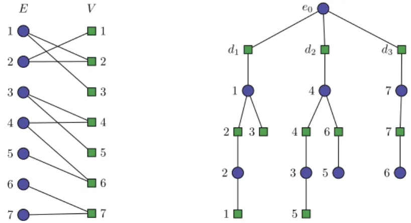
This yields a bipartite graph that is a single tree. Note that the nodes along a path from the root to any other node are alternately hyperedge/vertex nodes. Assume we “unfold” this tree in order to draw the bipartite graph in a layered manner, as illustrated in Figure 1.
Our dynamic program processes the unfolded treeT in a bottom-up manner. It consists of two separate dynamic programs, one for the hyperedges, and one for the vertices. We describe these programs informally in this section (technical details of the dynamic program will be given in the full version).
Consider an arbitrary subtree inT rooted at either a node represented by a hyperedge or vertex. Both dynamic programs rely on the fact that a subset of this subtree can be solved to optimality, which immediately can be used to solve a greater subset to optimality. In case the subtree is rooted at a node represented by a hyperedge, we consider the subtree up until the first schildren in the subtree of the hyperedge. Once the optimal solutions (minimum required cost to obtain a specific profit, if possible) are known for every possible profit (upper bounded bynP), it is possible to find optimal solutions for the subtree until the firsts+ 1 children by linear enumeration. A similar, but slightly adapted method works in case the subtree is rooted by a vertex rather than a hyperedge.
1 2 3 4 5 6 7 1 2 3 4 5 6 7 E V e0 d1 d2 d3 1 4 7 2 3 4 6 7 2 3 5 6 1 5
Figure 1Example of a incidence graph (left) and its “unfolded’ tree (right).
Furthermore, we can employ standard techniques (profit truncation) to turn the above pseudo-polynomial time algorithm into an FPTAS, i.e., an algorithm that takes an error parameter ε > 0 and computes in time polynomial in the input size and 1/ε a (1− ε)-approximation to the optimal solution.
ITheorem 11. There exists an FPTAS for GBMC-Forestthat runs in timeO(mn5/2).
6
GBMC with a bounded size feedback vertex set
We have shown in the previous section that GBMC-Forest can be solved in pseudo-polynomial time and that there is an FPTAS. This implies that the inapproximability of the general problem is caused by the cycles in the incidence graph. In this section, we provide a fixed parameter tractability result that allows us to handle incidence graphs with cycles. The fixed parameter is the minimum numberαof hyperedge nodes that we need to remove in order to make the incidence graph acyclic.
To provide an initial intuition, construct a graph G0= (E, E0) where every hyperedge e∈E is represented by a node, and two nodes are connected if and only if the corresponding hyperedges share at least one element. This defines the edge set E0 in the new graph. Consider the case in whichGcontains solely one cycle. Select a hyperedge node of the cycle and fix whether this hyperedge is chosen or not in a solution (i.e., setx= 0 or 1). We then consider the reduced problem in which hyperedgeeis removed. The incidence graph of the reduced problem is a forest and can thus be solved optimally by using the pseudo-polynomial time algorithm (or approximately by using the FPTAS) of the previous section. Solving this
GBMC-Forestproblem for every possible choice of hyperedge to remove, and taking the best solution, yields a solution to the general GBMC problem for the instance with one cycle. Thus, if the graph contains one cycle, the running time is multiplied by 2. We can extend this idea to more general graphs.
Define αas the minimum number of hyperedges whose removal turn the graph into a forest, i.e.,αis the cardinality of theminimum feedback vertex subsetof the hyperedge nodes of the incidence graph. We refer to the latter as theminimum feedback hyperedge node set. Then the running time of the algorithms mentioned in the previous sections is multiplied by a factor of 2α, because it is necessary to solve the problem on a forest for every combination
on thoseαhyperedges.
The problem of finding a minimum feedback vertex set is NP-hard in general, but it is fixed parameter tractable. Cao et al. [2] give an O(3.83ααn2) time algorithm to solve the
1 2 3 4 5 1 2 3 4 5 E V 1 2 3 4 5
Figure 2Example of a transformation to the feedback vertex set problem.
problem, wherenhere refers to the number of nodes in the graph. We use this to prove the following theorem.
ITheorem 12. GBMC is solvable in O(mn3P22α+ 3.83ααm2)time, where αis the size
of the minimum feedback hyperedge node set.
All that needs to be shown is how to use theO(3.83ααn2) algorithm of [2] in order to find a minimum feedback vertex set restricted to only the hyperedge nodes of the incidence graph. This is straightforward: We reduce the incidence graph ofGto the aforementioned multigraphG0 = (E, E0) with onlyE as its vertex set. The edge set E0 is constructed as follows: there exists an edge between two hyperedges if they share at least one vertex in the original graph. It is now easy to see that there is a one-to-one correspondence between the cycles in the incidence graph ofGand the cycles inG0, and each cycle in the incidence graph ofGcorresponds to a cycle inG0 on the same set of vertices. Therefore, a minimum feedback vertex set ofG0 corresponds to a minimum feedback hyperedge node set ofG, and the algorithm of Cao et al. will find such a set inO(3.83ααn2) time.
The transformation is illustrated in Figure 2. There, hyperedge 3 and 5 are connected by vertex 4 in (the incidence graph representation of)G, thus an edge {3,5} is added in G0. The edge labels are omitted. Note that hyperedge 4 and 5 are connected by two edges, because they are both connected to vertex 4 and vertex 5.
7
Conclusions
In this paper we have presented various approximation algorithms for important special cases of the GBMC problem. Clearly, the most interesting open problem that remains to be solved is whether there exists a constant factor approximation algorithm for the general GBMC problem that runs in polynomial-time. Such a result would form a very interesting contrast with the inapproximability result for the problem of submodular function maximization with a submodular budget constraint under the oracle access model, which we mentioned in the introduction.
An interesting and challenging intermediate goal would be to find a constant factor approximation algorithm for the case that the hyperedges have a fixed sizek. AlgorithmA
References
1 G. Calinescu, C. Chekuri, M. Pál, and J. Vondrák. Maximizing a monotone submodular function subject to a matroid constraint. SIAM Journal on Computing, 40(6):1740–1766, 2011.
2 Y. Cao, J. Chen, and Y. Liu. On feedback vertex set new measure and new structures. In Proceedings of the 12th Scandinavian conference on Algorithm Theory, pages 93–104. Springer-Verlag, 2010.
3 R. Cohen and L. Katzir. The generalized maximum coverage problem. Information Pro-cessing Letters, 108(1):15–22, 2008.
4 U. Feige. A threshold of ln n for approximating set cover. Journal of the ACM, 45(4):634– 652, 1998.
5 J. Feldman, S. Muthukrishnan, M. Pál, and C. Stein. Budget optimization in search-based advertising auctions. In Proceedings of the 8th ACM conference on electronic commerce, pages 40–49, New York, NY, USA, 2007. ACM.
6 D.S. Hochbaum, editor.Approximation Algorithms for NP-hard Problems. PWS Publishing Co., 1997.
7 R.K. Iyer and J.A. Bilmes. Submodular optimization with submodular cover and submod-ular knapsack constraints. In Advances in Neural Information Processing Systems, pages 2436–2444. MIT Press, 2013.
8 H. Kellerer, U. Pferschy, and D. Pisinger. Knapsack Problems. Springer-Verlag, 2004. 9 S. Khuller, A. Moss, and J. Naor. The budgeted maximum coverage problem. Information
Processing Letters, 70(1):39–45, 1999.
10 Z. Svitkina and L. Fleischer. Submodular approximation: Sampling-based algorithms and lower bounds. SIAM Journal of Computing, 40(6):1715–1737, 2011.