Towards Practical Theory: Bayesian Optimization and Optimal Exploration

Computer Science and Artificial Intelligence Laboratory

Technical Report

MIT-CSAIL-TR-2016-006

May 26, 2016

Towards Practical Theory: Bayesian

Optimization and Optimal Exploration

Towards Practical Theory: Bayesian Optimization

and Optimal Exploration

by

Kenji Kawaguchi

Submitted to the Department of Electrical Engineering and Computer

Science

in partial fulfillment of the requirements for the degree of

Master of Science

at the

MASSACHUSETTS INSTITUTE OF TECHNOLOGY

February 2016

c

Massachusetts Institute of Technology 2016. All rights reserved.

Author . . . .

Department of Electrical Engineering and Computer Science

January 15, 2016

Certified by. . . .

Leslie P. Kaelbling

Professor of Computer Science and Engineering

Thesis Supervisor

Certified by. . . .

Tomas Lozano-Perez

Professor of Computer Science and Engineering

Thesis Supervisor

Accepted by . . . .

Professor Leslie A. Kolodziejski

Chair of the Committee on Graduate Students

Towards Practical Theory: Bayesian Optimization and

Optimal Exploration

by

Kenji Kawaguchi

Submitted to the Department of Electrical Engineering and Computer Science on January 15, 2016, in partial fulfillment of the

requirements for the degree of Master of Science

Abstract

This thesis discusses novel principles to improve the theoretical analyses of a class of methods, aiming to provide theoretically driven yet practically useful methods. The thesis focuses on a class of methods, called bound-based search, which includes several planning algorithms (e.g., the A* algorithm and the UCT algorithm), sev-eral optimization methods (e.g., Bayesian optimization and Lipschitz optimization), and some learning algorithms (e.g., PAC-MDP algorithms). For Bayesian optimiza-tion, this work solves an open problem and achieves an exponential convergence rate. For learning algorithms, this thesis proposes a new analysis framework, called PAC-RMDP, and improves the previous theoretical bounds. The PAC-RMDP framework also provides a unifying view of some previous near-Bayes optimal and PAC-MDP algorithms. All proposed algorithms derived on the basis of the new principles pro-duced competitive results in our numerical experiments with standard benchmark tests.

Thesis Supervisor: Leslie P. Kaelbling

Title: Professor of Computer Science and Engineering Thesis Supervisor: Tomas Lozano-Perez

Acknowledgments

I would like to express my sincere gratitude to my advisors Prof. Leslie Kaelbling and Prof. Tomás Lozano-Pérez, for all of their support and keen insights. In addition to the technical input provided by them, my experience of their quick, flexible, and profound thinking and discussions has been valuable, providing a sense of successful research styles that I could learn from.

Further, I would like to thank Dr. Remi Munos for his thoughtful comments and suggestions for my work on Bayesian optimization. Without his previous work on optimistic optimization, this work could not have been completed.

I would also like to thank Prof. Michael Littman for his thoughtful comments on and suggestions for my work on optimal exploration in MDP. His suggestions and encouraging comments motivated me to complete the work.

Next, I would like to acknowledge Funai Overseas Scholarship for their very gen-erous financial support and for providing me with a scientific community active in universities across the world.

Finally, I would thank my wife Molly Kruko for her support and happy moments that we share, which have been a vital source of motivation and relaxation to me while completing this work.

Contents

1 Introduction 13

1.1 Bayesian Optimization . . . 15

1.2 Learning/Exploration in MDPs . . . 16

2 Bayesian Optimization with Exponential Convergence 19 2.1 Gaussian Process Optimization . . . 19

2.2 Infinite-Metric GP Optimization . . . 21

2.2.1 Overview . . . 21

2.2.2 Description of Algorithm . . . 22

2.2.3 Technical Detail of Algorithm . . . 24

2.2.4 Relationship to Previous Algorithms . . . 26

2.3 Analysis . . . 27

2.4 Experiments . . . 32

3 Bounded Optimal Exploration in MDP 35 3.1 Preliminaries . . . 35

3.2 Bounded Optimal Learning . . . 37

3.2.1 Reachability in Model Learning . . . 37

3.2.2 PAC in Reachable MDP . . . 38

3.3 Discrete Domain . . . 40

3.3.1 Algorithm . . . 40

3.3.2 Analysis . . . 41

3.4 Continuous Domain . . . 45

3.4.1 Algorithm . . . 46

3.4.2 Analysis . . . 47

3.4.3 Experimental Examples . . . 48

4 Conclusion 53 A Appendix – Bayesian Optimization 55 A.1 Proofs for Family of Division Procedures . . . 56

A.2 Proofs for a Concrete Division Procedure . . . 61

B Appendix – Exploration in MDP 63 B.1 Proofs of Propositions 1 and 2 . . . 63

B.2 Relationship to Bounded Rationality and Bounded Optimality . . . . 64

B.3 Corresponding Notions of Regret and Average Loss . . . 65

B.4 Proofs of Theoretical Results for Algorithm 3.1 . . . 66

B.5 Additional Experimental Example for Discrete Domain . . . 72

B.6 Proofs of Theoretical Results for Algorithm 3.2 . . . 72

List of Figures

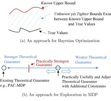
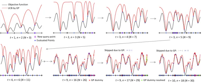
1-1 Two distinct approaches to improve the theory for bound-based search methods: For Bayesian optimization, I have leveraged existence of un-known yet tighter bounds. For the MDP exploration problem, I have proposed an adjustable theoretical guarantee to accommodate practi-cal needs. . . 15 2-1 An illustration of IMGPO: tis the number of iteration, nis the number

of divisions (or splits), N is the number of function evaluations. . . . 24

2-2 Performance Comparison: in the order, the digits inside of the paren-theses [ ] indicate the dimensionality of each function, and the variables

ˉ

ρt and Ξn at the end of computation for IMGPO. . . 31

2-3 Sin1000: [D = 1000, ρˉ= 3.95, Ξn =4] . . . 32

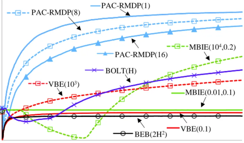
3-1 Average total reward per time step for the Chain Problem. The algo-rithm parameters are shown as PAC-RMDP(h), MBIE(, δ), VBE(δ),

BEB(β), and BOLT(η). . . 45

3-2 Total reward per episode for the mountain car problem with PAC-RMDP(h) and PAC-MDP(). . . 50

3-3 Total reward per episode for the HIV problem with PAC-RMDP(h)

and PAC-MDP(). . . 50

B-1 Average total reward per time step for the Chain Problem. The algo-rithm parameters are shown as PAC-RMDP(h), MBIE(, δ), VBE(δ),

B-2 Average total reward per time step for the modified Chain Problem. The algorithm parameters are shown as PAC-RMDP(h), MBIE(, δ),

List of Tables

Chapter 1

Introduction

“In theory, there is no difference between theory and practice. But, in practice, there is.”– Jan L. A. van de Snepscheut. One of the reasons why theory and practice can diverge is that a set of assumptions made in theory can be invalid in practice. The well-known spherical cow metaphor exemplifies this phenomenon (i.e., theoretical results based on the assumptions of the spherical shape and the vacuum condition may not be directly useful in practice for farmers). Indeed, it is well recognized that we should carefully select a set of valid assumptions that hold in practice. However, selecting a set of valid assumptions is often not sufficient to prevent the divergence of theory and practice. The divergence can occur when a set of assumptions are not sufficiently sharp (or tight) to exclude irrelevant problems or phenomena while capturing the class of the problems at hand.

In this thesis, I first identify a class of methods that has suffered from this sharp-ness issue at an algorithmic level, resulting in the divergence of theory and practice. I refer to the identified method class as bound-based search, which includes the A* search, Upper Confidence for Trees (UCT), and Forward Search Sparse Sampling (FSSS) algorithms [50]; exploration in Markov decision processes (MDPs) with opti-mism in the face of uncertainty [19]; Lipschitz optimization [37, 24, 7]; and Bayesian optimization with an upper confidence bound [41, 10]. Bound-based search methods have a common property: The tightness of the bound determines its effectiveness. The tighter the bound is, the better is the performance. However, it is often difficult

to obtain a tight bound while maintaining correctness in a theoretically supported manner. For example, in A* search, admissible heuristics maintain the correctness of the bound, but the estimated bound with admissibility is often very loose in prac-tice, resulting in long execution times for global search. This has seemingly lead to the divergence of theoretically driven approaches (that focus more on global search, maintaining theoretical guarantees yet taking a long time to converge in practice) and practically driven ones (that focus more on local search, obtaining a reasonable solution within a short time but with no global theoretical guarantee).

In this study, I have focused on two members of the class of bound-based search methods—Bayesian optimization and PAC–MDP algorithms—and proposed a spe-cific solution for each one to tighten their bounds with sharper assumptions, aiming to provide theoretically driven algorithms that perform well in practice.

Our two high-level approaches are illustrated in Figure 1-1. For the approach shown in Figure 1-1 (a), note thattighter yetunknown bounds exist unless the known bound is exact. We propose a way to additionally take advantage of this simple fact that has been overlooked in previous work. A high-level idea is the following. When we rely on a single known bound, the set of the next evaluation candidates is totally ordered in terms of the possible improvements with respect to the bound. In contrast, we consider a set of unknown tighter bounds (possibly uncountable), and as a result, the set of the next evaluation candidates can be partially ordered but not totally ordered in terms of the improvements with respect to the set of the bounds. Thus, we simultaneously evaluates several minimal (or maximal) elements of the partially ordered set to account for the existence of the unknown yet tighter bounds.

Another approach, illustrated in Figure 1-1 (b), is based on two ideas. First, there exist practical constraints that the current theory ignores. Because of that, what the current theory guarantees (the leftmost circle in Figure 1-1 (b)) can be considerably stronger than necessary (the red line in Figure 1-1 (b)). This has been a partial cause of loose theoretical bounds and impractical algorithms. Thus, we reduce the size of the practically irrelevant region in the scope of theoretical analyses. Second, we propose a way to adjust the degree of theoretical guarantees in order to achieve

(a) An approach for Bayesian Optimization

Stronger Theoretical Guarantee

Weaker Theoretical Guarantee

Existing Theoretical Guarantee e.g., PAC-MDP

Practically Usefully and Adjustable Theoretical Guarantee

with Additional Constraints

Practically Strongest Guarantee

(b) An approach for Exploration in MDP

Figure 1-1: Two distinct approaches to improve the theory for bound-based search methods: For Bayesian optimization, I have leveraged existence of unknown yet tighter bounds. For the MDP exploration problem, I have proposed an adjustable theoretical guarantee to accommodate practical needs.

the practicality that we want (the right circle in Figure 1-1 (b)).

1.1 Bayesian Optimization

I consider a general constrained global optimization problem: maximize f(x) subject

to x ∈ Ω ⊂ RD_{, where f : Ω → R denotes a non-convex black-box deterministic}

function. Such a problem arises in many real-world applications, such as parameter tuning in machine learning [39], engineering design problems [8], and model parameter fitting in biology [55]. For this problem, one performance measure of an algorithm is thesimple regret,rn, which is given by rn= supx∈Ωf(x)−f(x+)wherex+ is the best

input vector found by the algorithm. For brevity, I use the term “regret" to mean simple regret.

The general global optimization problem is known to be intractable if we make no further assumptions [11]. The simplest additional assumption to restore tractability

is to assume the existence of a bound on the slope of f. A well-known variant of

this assumption is Lipschitz continuity with a known Lipschitz constant, and many algorithms have been proposed in this setting [37, 28, 30]. These algorithms success-fully guarantee certain bounds on the regret. However appealing from a theoretical point of view, a practical concern was soon raised regarding the assumption that a tight Lipschitz constant is known. Some researchers relaxed this somewhat strong assumption by proposing procedures for estimating a Lipschitz constant during the optimization process [47, 24, 7].

Bayesian optimization is an efficient way to relax this assumption of the com-plete knowledge of the Lipschitz constant, and has become a well-recognized method for solving global optimization problems with non-convex black-box functions. In the machine learning community, Bayesian optimization, particularly by means of a Gaussian process (GP), is an active research area [14, 52, 41]. With the requirement of the access to theδ-cover sampling procedure (which samples the function uniformly

such that the density of the samples doubles in the feasible regions at each iteration), De Freitas et al. [10] recently proposed a theoretical procedure that maintains an exponential convergence rate (exponential regret). However, as pointed out by Wang et al. [51], the δ-cover sampling procedure is somewhat impractical. Accordingly,

their paper states that one remaining problem is to derive a GP-based optimization method with an exponential convergence ratewithout theδ-cover sampling procedure.

In this thesis, I propose a novel GP-based global optimization algorithm, which maintains an exponential convergence rate and converges rapidly without the δ

-cover sampling procedure. These results are described in Chapter 2 and a published paper [20].

1.2 Learning/Exploration in MDPs

The formulation of sequential decision making as an MDP has been successfully applied to a number of real-world problems. MDPs provide the ability to design adaptable agents that can operate effectively in uncertain environments. In many

situations, the environment that we wish to model has unknown aspects, and there-fore, the agent needs to learn an MDP by interacting with the environment. In other words, the agent has to explore the unknown aspects of the environment to learn the MDP. A considerable amount of theoretical work on MDPs has focused on efficient exploration, and a number of principled methods have been derived with the aim of learning an MDP to obtain a near-optimal policy. For example, Kearns and Singh [22] and Strehl and Littman [43] considered discrete state spaces, whereas Bernstein and Shimkin [5] and Pazis and Parr [33] examined continuous state spaces.

In practice, however, heuristics are still commonly used [26]. This is partly be-cause theoretically-driven methods tend to result in over-exploration. The focus of theoretical work (learning a near-optimal policy within a polynomial but long period of time) has apparently diverged from practical needs (learning a satisfactory policy within a reasonable period of time). In this thesis, I have modified the prevalent theo-retical approach to develop theotheo-retically-driven methods that come close to practical needs. These results are described in Chapter 2 and a published paper [18].

Chapter 2

Bayesian Optimization with

Exponential Convergence

This chapter presents a Bayesian optimization method with exponential convergence

without the need of auxiliary optimization and without the δ-cover sampling. Most

Bayesian optimization methods require auxiliary optimization: an additional non-convex global optimization problem, which can be time-consuming and hard to im-plement in practice. Also, the existing Bayesian optimization method with exponen-tial convergence [10] requires access to the δ-cover sampling, which was considered to

be impractical [10, 51]. Our approach eliminates both requirements and achieves an exponential convergence rate.

2.1 Gaussian Process Optimization

In Gaussian process optimization, we estimate the distribution over function f and

use this information to decide which point of f should be evaluated next. In a

parametric approach, we consider a parameterized function f(x; θ), with θ being

distributed according to some prior. In contrast, the nonparametric GP approach directly puts the GP prior over f as f(∙)∼GP(m(∙), κ(∙,∙)) wherem(∙)is the mean

function and κ(_∙,_∙)is the covariance function or the kernel. That is, m(x) =E[f(x)]

model is simply a joint Gaussian: f(x_1:N)_{∼ N}(m(x_1:N),K), where Ki,j = κ(xi, xj)

and N is the number of data points. To predict the value of f at a new data point,

we first consider the joint distribution over f of the old data points and the new data

point:   f(x1:N) f(xN+1)  _{∼ N}   m(x1:N) m(xN+1) ,   K k kT _κ(x N+1, xN+1)    

wherek=κ(x1:N,xN+1)∈RN×1. Then, after factorizing the joint distribution using

the Schur complement for the joint Gaussian, we obtain the conditional distribution, conditioned on observed entities _DN := {x1:N,f(x_1:N)}and xN+1, as:

f(xN+1)|DN, xN+1 ∼ N(μ(xN+1|DN), σ2(xN+1|DN))

where μ(xN+1|DN) = m(xN+1) +kTK−1(f(x_1:N) −m(x_1:N)) and σ2(xN+1|DN) =

κ(xN+1,xN+1)−kTK−1k. One advantage of GP is that this closed-form solution

simplifies both its analysis and implementation.

To use a GP, we must specify the mean function and the covariance function. The mean function is usually set to be zero. With this zero mean function, the conditional meanμ(xN+1|DN) can still be flexibly specified by the covariance function, as shown

in the above equation for μ. For the covariance function, there are several common

choices, including the Matern kernel and the Gaussian kernel. For example, the Gaussian kernel is defined as κ(x, x0_{) = exp−}1

2(x−x0) T

Σ−1_(x−x0_{) where Σ}−1

is the kernel parameter matrix. The kernel parameters or hyperparameters can be estimated by empirical Bayesian methods [32]; see [35] for more information about GP.

The flexibility and simplicity of the GP prior make it a common choice for con-tinuous objective functions in the Bayesian optimization literature. Bayesian opti-mization with GP selects the next query point that optimizes the acquisition function generated by GP. Commonly used acquisition functions include the upper confidence bound (UCB) and expected improvement (EI). For brevity, we consider Bayesian

op-timization with UCB, which works as follows. At each iteration, the UCB function _U is maintained as _U(x|DN) =μ(x|DN) +ςσ(x|DN) where ς ∈R is a parameter of the

algorithm. To find the next query xn+1 for the objective function f, GP-UCB solves

an additional non-convex optimization problem with _U asxN+1 = arg maxxU(x|DN).

This is often carried out by other global optimization methods such as DIRECT and CMA-ES. The justification for introducing a new optimization problem lies in the assumption that the cost of evaluating the objective function f dominates that of

solving additional optimization problem.

For deterministic function, de Freitas et al. [10] recently presented a theoretical procedure that maintains exponential convergence rate. However, their own paper and the follow-up research [10, 51] point out that this result relies on an impractical sampling procedure, the δ-cover sampling. To overcome this issue, Wang et al. [51]

combined GP-UCB with a hierarchical partitioning optimization method, the SOO algorithm [31], providing a regret bound with polynomial dependence on the number of function evaluations. They concluded that creating a GP-based algorithm with an

exponential convergence rate without the impractical sampling procedure remained an open problem.

2.2 Infinite-Metric GP Optimization

2.2.1 Overview

The GP-UCB algorithm can be seen as a member of the class of bound-based search methods, which includes Lipschitz optimization, A* search, and PAC-MDP algo-rithms with optimism in the face of uncertainty. As discussed in section 1, it is often difficult to obtain a tight bound for bound-based methods, resulting in a long period of global search or heuristic approach with no theoretical guarantee.

The GP-UCB algorithm has the same problem. The bound in GP-UCB is rep-resented by UCB, which has the following property: f(x) ≤ U(x|D) with some

probability. I formalize this property in the analysis of our algorithm. The prob-lem is essentially due to the difficulty of obtaining a tight bound _U(x|D) such that

f(x) _{≤ U}(x_|D) and f(x) _{≈ U}(x_|D) (with some probability). Our solution strategy

is to first admit that the bound encoded in GP prior may not be tight enough to be useful by itself. Instead of relying on a single bound given by the GP, I leverage the existence of an unknown bound encoded in the continuity at a global optimizer.

Assumption 2.1. (Unknown Bound) There exists a global optimizer x∗ and an

unknown semi-metric`such that for allx<sub>∈</sub>Ω,f(x∗<sub>)≤f(x)+`(x, x</sub>∗_{)and`(x, x}∗_)<

∞.

In other words, we do not expect the known upper bound due to GP to be tight, but instead expect that there exists some unknown bound that might be tighter. No-tice that in the case where the bound by GP is as tight as the unknown bound by semi-metric ` in Assumption 2.1, our method still maintains an exponential

conver-gence rate and an advantage over GP-UCB (no need for auxiliary optimization). Our method is expected to become relatively much better when the known bound due to GP is less tight compared to the unknown bound by `.

As the semi-metric ` is unknown, there are infinitely many possible candidates

that we can think of for `. Accordingly, we simultaneously conduct global and local

searches based on all the candidates of the bounds. The bound estimated by GP is used to reduce the number of candidates. Since the bound estimated by GP is known, we can ignore the candidates of the bounds that are looser than the bound estimated by GP. The source code of the proposed algorithm is publicly available at

http://lis.csail.mit.edu/code/imgpo.html.

2.2.2 Description of Algorithm

Figure 2-1 illustrates how the algorithm works with a simple 1-dimensional objec-tive function. We employ hierarchical partitioning to maintain hyperintervals, as illustrated by the line segments in the figure. We consider a hyperrectangle as our hyperinterval, with its center being the evaluation point of f (blue points in each line

procedure for each interval size:

(i) Select the interval with the maximum center value among the intervals of the same size.

(ii) Keep the interval selected by (i) if it has a center value greater than that of any

larger interval.

(iii) Keep the interval accepted by (ii) if it contains a UCB greater than the center value of any smaller interval.

(iv) If an interval is accepted by (iii), divide it along with the longest coordinate into three new intervals.

(v) For each new interval, if the UCB of the evaluation point is less than the best function value found so far, skip the evaluation and use the UCB value as the center value until the interval is accepted in step (ii) on some future iteration; otherwise, evaluate the center value.

(vi) Repeat steps (i)–(v) until every size of intervals are considered

Then, at the end of each iteration, the algorithm updates the GP hyperparameters. Here, the purpose of steps (i)–(iii) is to select an interval that might contain the global optimizer. Steps (i) and (ii) select the possible intervals based on the unknown bound by `, while Step (iii) does so based on the bound by GP.

I now explain the procedure using the example in Figure 2-1. Let nbe the number

of divisions of intervals and let N be the number of function evaluations. t is the

number of iterations. Initially, there is only one interval (the center of the input region

Ω_⊂R) and thus this interval is divided, resulting in the first diagram of Figure 2-1.

At the beginning of iterationt= 2, step (i) selects the third interval from the left side

in the first diagram (t = 1, n = 2), as its center value is the maximum. Because there

are no intervals of different size at this point, steps (ii) and (iii) are skipped. Step (iv) divides the third interval, and then the GP hyperparameters are updated, resulting in the second diagram (t = 2, n = 3). At the beginning of iteration t = 3, it starts

Figure 2-1: An illustration of IMGPO: t is the number of iteration, n is the number

of divisions (or splits), N is the number of function evaluations.

conducting steps (i)–(v) for the largest intervals. Step (i) selects the second interval from the left side and step (ii) is skipped. Step (iii) accepts the second interval, because the UCB within this interval is no less than the center value of the smaller intervals, resulting in the third diagram (t = 3, n = 4). Iteration t = 3 continues by

conducting steps (i)–(v) for the smaller intervals. Step (i) selects the second interval from the left side, step (ii) accepts it, and step (iii) is skipped, resulting in the forth diagram (t = 3, n = 4). The effect of the step (v) can be seen in the diagrams for

iterationt= 9. Atn = 16, the far right interval is divided, but no function evaluation

occurs. Instead, UCB values given by GP are placed in the new intervals indicated by the red asterisks. One of the temporary dummy values is resolved at n = 17when the

interval is queried for division, as shown by the green asterisk. The effect of step (iii) for the rejection case is illustrated in the last diagram for iteration t = 10. Atn= 18,

t is increased to 10 from 9, meaning that the largest intervals are first considered for

division. However, the three largest intervals are all rejected in step (iii), resulting in the division of a very small interval near the global optimum at n= 18.

2.2.3 Technical Detail of Algorithm

I define h to be the depth of the hierarchical partitioning tree, and ch,i to be

the center point of the ith _{hyperrectangle at depth h. N}

Algorithm 2.1. Infinite-Metric GP Optimization (IMGPO)

Input: an objective function f, the search domainΩ, the GP kernelκ,Ξmax∈N+ andη ∈(0,1)

1: Initialize the set _Th={∅} ∀h≥0

2: Setc0,0 to be the center point of ΩandT0← {c0,0} 3: Evaluate f atc0,0: g(c0,0)←f(c0,0) 4: f+ ←g(c0,0),D ← {(c0,0, g(c0,0))} 5: n, N←1, Ngp ←0,Ξ←1 6: fort= 1,2,3, ...do 7: υmax← −∞

8: forh= 0todepth(_T)do #for-loop for steps (i)-(ii)

9: whiletruedo

10: i∗

h← arg maxi:ch,i∈Thg(ch,i)

11: if g(ch,i∗

h)< υmax then

12: i∗

h← ∅,break

13: else if g(ch,i∗

h)isnot labeled asGP-based then

14: υmax←g(ch,i∗

h),break

15: else

16: g(ch,i∗

h)←f(ch,i∗h)and remove theGP-based label from g(ch,i∗h)

17: N _←N+ 1, Ngp←Ngp−1

18: D ← {D,(ch,i∗

h, g(ch,i∗h))}

19: forh= 0todepth(_T)do #for-loop for step (iii)

20: if i∗

h6=∅ then

21: ξ← the smallest positive integer s.t. i∗h+ξ =6 ∅ andξ≤min(Ξ,Ξmax)if exists, and 0

otherwise 22: z(h, i∗h) = maxk:ch+ξ,k∈Th0+ξ(ch,i∗ h)U (ch+ξ,k|D) 23: if ξ6= 0 andz(h, i∗h)< g(ch+ξ,i∗ h+ξ)then 24: i∗ h← ∅,break 25: υmax← −∞

26: forh= 0todepth(_T)do #for-loop for steps (iv)-(v)

27: if i∗

h6=∅ andg(ch,i∗

h)≥υmax then

28: n←n+ 1.

29: Divide the hyperrectangle centered atch,i∗

h along with the longest coordinate into three

new hyperrectangles with the following centers:

S={ch+1,i(lef t), ch+1,i(center), ch+1,i(right)} 30: _Th+1← {Th+1,S}

31: Th← Th\ch,i∗

h, g(ch+1,i(center))←g(ch,i∗h)

32: forinew={i(lef t), i(right)}do

33: if U(ch+1,inew|D)≥f

+ _then 34: g(ch+1,inew)←f(ch+1,inew)

35: _{D ← {D},(ch+1,inew, g(ch+1,inew))}

N←N+ 1, f+_←max(f+_{, g(c}

h+1,inew)),υmax= max(υmax, g(ch+1,inew))

36: else

37: g(ch+1,inew)← U(ch+1,inew|D)and labelg(ch+1,inew)asGP-based.

Ngp←Ngp+ 1

38: UpdateΞ: if f+ _{was updated,Ξ}

←Ξ + 22 _{, and otherwise,Ξ}

←max(Ξ−2−1_,1) 39: Update GP hyperparameters by an empirical Bayesian method

evaluations. Define depth(_T) to be the largest integer h such that the set _Th is not

empty. To compute UCB _U, I use ςM = p

2 log(π2_M2_/12η) where _M is the number

of the calls made so far for _U (i.e., each time we use _U, we increment M by one).

This particular form of ςM is to maintain the property of f(x) ≤ U(x|D) during an

execution of our algorithm with probability at least 1₋η. Here, η is the parameter

of IMGPO. Ξmax is another parameter, but it is only used to limit the possibly long

computation of step (iii) (in the worst case, step (iii) computes UCBs 3Ξmax times although it would rarely happen).

The pseudocode is shown in Algorithm 2.1. Lines 8 to 23 correspond to steps (i)-(iii). These lines compute the index i∗

h of the candidate of the rectangle that may

contain a global optimizer for each depth h. For each depth h, non-null index i∗ h

at Line 24 indicates the remaining candidate of a rectangle that we want to divide. Lines 24 to 33 correspond to steps (iv)-(v) where the remaining candidates of the rectangles for all hare divided. To provide a simple executable division scheme (line

29), we assume Ω to be a hyperrectangle (see the last paragraph of section 4 for a

general case).

Lines 8 to 17 correspond to steps (i)-(ii). Specifically, line 10 implements step (i) where a single candidate is selected for each depth, and lines 11 to 12 conduct step (ii) where some candidates are screened out. Lines 13 to 17 resolve the temporary dummy values computed by GP. Lines 18 to 23 correspond to step (iii) where the candidates are further screened out. At line 21, _T0

h+ξ(ch,i∗

h) indicates the set of all center points of a fully expanded tree until depth h+ξ within the region covered by

the hyperrectangle centered at ch,i∗

h. In other words, T 0

h+ξ(ch,i∗

h)contains the nodes of the fully expanded tree rooted at ch,i∗

h with depthξ and can be computed by dividing the current rectangle at ch,i∗

h and recursively divide all the resulting new rectangles until depth ξ (i.e., depth ξ fromch,i∗

h, which is depth h+ξ in the whole tree).

2.2.4 Relationship to Previous Algorithms

The most closely related algorithm is the BaMSOO algorithm [51], which combines SOO with GP-UCB. However, it only achieves a polynomial regret bound while

IMGPO achieves a exponential regret bound. IMGPO can achieve exponential regret because it utilizes the information encoded in the GP prior/posterior to reduce the degree of the ignorance of the unknown assumption with the semi-metric `.

The idea of considering a set of infinitely many bounds was first proposed by Jones et al. [16]. Their DIRECT algorithm has been successfully applied to real-world problems [8, 55], but it only maintains the consistency property (i.e., convergence in the limit) from a theoretical viewpoint. DIRECT takes an input parameter to

balance the global and local search efforts. This idea was generalized to the case of an unknown semi-metric and strengthened with a theoretical support (finite regret bound) by Munos [31] in the SOO algorithm. By limiting the depth of the search tree with a parameter hmax, the SOO algorithm achieves a finite regret bound that

depends on the near-optimality dimension.

2.3 Analysis

In this section, I prove an exponential convergence rate of IMGPO and theoretically discuss the reason why the novel idea underling IMGPO is beneficial. The proofs are provided in the supplementary material. To examine the effect of considering infinitely many possible candidates of the bounds, I introduce the following term.

Definition 2.1. (Infinite-metric exploration loss). The infinite-metric exploration loss ρt is the number of intervals to be divided during iteration t.

The infinite-metric exploration loss ρτ can be computed as ρt = Pdepth_h=1 (T)1(i∗h 6=∅)

at line 25. It is the cost (in terms of the number of function evaluations) incurred by not committing to any particular upper bound. If we were to rely on a specific bound, ρτ would be minimized to 1. For example, the DOO algorithm [31] has

ρt = 1 ∀t ≥ 1. Even if we know a particular upper bound, relying on this knowledge

and thus minimizing ρτ is not a good option unless the known bound is tight enough compared to the unknown bound leveraged in our algorithm. This will be clarified in our analysis. Let ρˉt be the maximum of the averages of ρ1:t0 for t0 = 1,2, ..., t (i.e.,

ˉ

ρt≡max({_t10

Pt0

τ=1ρτ ; t0 = 1,2, ..., t}).

Assumption 2.2. For some pair of a global optimizer x∗ _{and an unknown} semi-metric ` that satisfies Assumption 1, both of the following, (i) shape on ` and (ii)

lower bound constant, conditions hold:

(i) there exist L > 0, α >0 and p _≥1 in R such that for all x, x0 _{∈Ω, `(x}0_{, x)≤}

L||x0−x||α p.

(ii) there exists θ _∈(0,1) such that for all x_∈Ω, f(x∗_{)≥f(x) +θ`(x, x}∗_).

In Theorem 2.1, I show that the exponential convergence rate O λN+Ngpwith _{λ <1} is achieved. I define Ξn ≤ Ξmax to be the largest ξ used so far with n total node

expansions. For simplicity, we assume that Ω is a square, which we satisfied in our

experiments by scaling original Ω.

Theorem 2.1. Assume Assumptions 2.1 and 2.2. Let β = supx,x0_∈Ω21kx −x0k∞.

Let λ= 3−2CDαρtˉ _<1. Then, with probability at least _1−η, the regret of IMGPO is

bounded as rN ≤L(3βD1/p)αexp −α N +Ngp 2CDρˉt − Ξn−2 ln 3 =O λN+Ngp_.

Importantly, our bound holds for the best values of the unknown L, α and p even

though these values are not given. The closest result in previous work is that of BaMSOO [51], which obtained _O˜_(n− 2α

D(4−α)) with probability 1−η forα={1,2}. As

can be seen, I have improved the regret bound. Additionally, in our analysis, we can see how L, p, and α affect the bound, allowing us to view the inherent difficulty of

an objective function in a theoretical perspective. Here, C is a constant in N and

is used in previous work [31, 51]. For example, if we conduct 2D _{or 3}D _{−1 function}

evaluations per node-expansion and if p=∞, we have that C = 1.

We note thatλcan get close to one as input dimensionDincreases, which suggests

strategy for addressing this problem would be to leverage additional assumptions such as those in [52, 17].

Remark 2.1. (The effect of the tightness of UCB by GP) If UCB computed by GP is “useful” such that N/ρˉt= Ω(N), then our regret bound becomes

O exp −N₂+_CDNgpαln 3 .

If the bound due to UCB by GP is too loose (and thus useless), ρˉt can increase

up to O(N/t) (due to ρˉt ≤ Pt_i=1i/t ≤ O(N/t)), resulting in the regret bound of

Oexp₋t(1+Ngp/N)

2CD αln 3

, which can be bounded by1

O exp −N +Ngp 2CD max( 1 √ N, t N)αln 3 .

Our proof works with this additional mechanism, but results in the regret bound with N being replaced by √N. Thus, if we assume to have at least “not useless”

UCBs such that N/ρˉt= Ω(

√

N), this additional mechanism can be disadvantageous.

Accordingly, we do not adopt it in our experiments.. This is still better than the known results.

Remark 2.2. (The effect of GP) Without the use of GP, our regret bound would be as follows: rN ≤ L(3βD1/p)αexp(−α[_2CDN _ρ˜1_t −2] ln 3), where ρˉt ≤ ρ˜t is the

infinite-metric exploration loss without GP. Therefore, the use of GP reduces the regret bound by increasing Ngp and decreasing ρˉt, but may potentially increase the bound

by increasing Ξn≤Ξ.

Remark 2.3. (The effect of infinite-metric optimization) To understand the effect of considering all the possible upper bounds, we consider the case without GP. If we con-sider all the possible bounds, we have the regret bound L(3βD1/p₎α_exp(−α[ N

2CD

1 ˜ ρt −

2] ln 3)for the best unknown L, α and p. For standard optimization with a estimated

Table 2.1: Average CPU time (in seconds) for the experiment with each test function Algorithm Sin1 Sin2 Peaks Rosenbrock2 Branin Hartmann3 Hartmann6 Shekel5 GP-PI 29.66 115.90 47.90 921.82 1124.21 573.67 657.36 611.01 GP-EI 12.74 115.79 44.94 893.04 1153.49 562.08 604.93 558.58 SOO 0.19 0.19 0.24 0.744 0.33 0.30 0.25 0.29 BaMSOO 43.80 4.61 7.83 12.09 14.86 14.14 26.68 371.36 IMGPO 1.61 3.15 4.70 11.11 5.73 6.80 13.47 15.92 bound, we have L0_(3βD1/p0 )α0 exp(₋α0_[ N

2C0_D −2] ln 3) for an estimated L0, α0, and p0.

By algebraic manipulation, considering all the possible bounds has a better regret when ˜ ρ−_t1 ≥ 2CD Nln 3α(( N 2C0_D −2) ln 3 α0 _{+ 2 ln 3}α_−lnL0(3βD1/p 0 )α0 L(3βD1/p₎α ).

For an intuitive insight, we can simplify the above by assuming α0 = α and C0 =C

as ˜ ρ−_t1 ≥1− Cc2D N ln L0Dα/p0 LDα/p .

Because L and p are the ones that achieve the lowest bound, the logarithm on the

right-hand side is always non-negative. Hence, ρ˜t = 1 always satisfies the condition.

When L0 _{and p}0 _{are not tight enough, the logarithmic term increases in magnitude,} allowing ρ˜t to increase. For example, if the second term on the right-hand side has

a magnitude of greater than 0.5, then ρ˜t= 2 satisfies the inequality. Therefore, even

if we know the upper bound of the function, we can see that it may be better not to rely on this, but rather take the infinite many possibilities into account.

One may improve the algorithm with different division procedures than one pre-sented in Algorithm 2.1. Accordingly, in the supplementary material, I derive an abstract version of the regret bound for IMGPO with a family of division proce-dures that satisfy some assumptions. This information could be used to design a new division procedure.

(a) Sin1: [1, 1.92, 2] (b) Sin2: [2, 3.37, 3]

(c) Peaks: [2, 3.14, 4] (d) Rosenbrock2: [2, 3.41, 4]

(e) Branin: [2, 4.44, 2] (f) Hartmann3: [3, 4.11, 3]

(g) Hartmann6: [6, 4.39, 4] (h) Shekel5: [4, 3.95, 4]

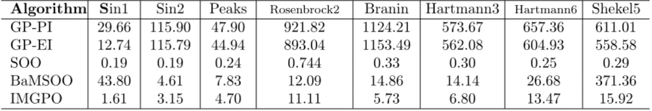
Figure 2-2: Performance Comparison: in the order, the digits inside of the parentheses [ ] indicate the dimensionality of each function, and the variables ρˉt and Ξn at the

Figure 2-3: Sin1000: [D = 1000, ρˉ=3.95, Ξn= 4]

2.4 Experiments

In this section, I compare the IMGPO algorithm with the SOO, BaMSOO, GP-PI and GP-EI algorithms [31, 51, 39]. In previous work, BaMSOO and GP-UCB were tested with a pair of a handpicked good kernel and hyperparameters for each function [51]. In our experiments, we assume that the knowledge of good kernel and hyperparameters is unavailable, which is usually the case in practice. Thus, for IMGPO, BaMSOO, GP-PI and GP-EI, we simply used one of the most popular kernels, the isotropic Matern kernel with ν = 5/2. This is given by κ(x, x0_{) = g(}p_5||x−x0_||2_/l), where

g(z) = σ2_{(1 + z +z}2_{/3) exp(−z). Then, I blindly initialized the hyperparameters}

to σ = 1 and l = 0.25 for all the experiments; these values were updated with an

empirical Bayesian method after each iteration. To compute the UCB by GP, I used

η= 0.05 for IMGPO and BaMSOO. For IMGPO, Ξmax was fixed to be22 (the effect

of selecting different values is discussed later). For BaMSOO and SOO, the parameter

hmax was set to√n, according to Corollary 4.3 in [31]. For GP-PI and GP-EI, I used

the SOO algorithm and a local optimization method using gradients to solve the auxiliary optimization. For SOO, BaMSOO and IMGPO, I used the corresponding deterministic division procedure (givenΩ, the initial point is fixed and no randomness

exists). For GP-PI and GP-EI, I randomly initialized the first evaluation point and report the mean and one standard deviation for 50 runs.

2-2 and 2-3. The vertical axis is log10(f(x∗)−f(x+)), wheref(x∗)is the global optima

and f(x+_{) is the best value found by the algorithm. Hence, the lower the plotted}

value on the vertical axis, the better the algorithm’s performance. The last five functions are standard benchmarks for global optimization [48]. The first two were used in [31] to test SOO, and can be written as fsin1(x) = (sin(13x) sin +1)/2 for

Sin1 and fsin2(x) = fsin1(x1)fsin1(x2) for Sin2. The form of the third function is

given in Equation (16) and Figure 2 in [29]. The last function in Figure 2-3 is Sin2 embedded in 1000 dimension in the same manner described in Section 4.1 in [52], which is used here to illustrate a possibility of using IMGPO as a main subroutine to scale up to higher dimensions with additional assumptions. For this function, I used REMBO [52] with IMGPO and BaMSOO as its Bayesian optimization subroutine. All of these functions are multimodal, except for Rosenbrock2, with dimensionality from 1 to 1000.

As we can see from Figure 2-2 and 2-3, IMGPO outperformed the other algorithms in general. SOO produced the competitive results for Rosenbrock2 because our GP prior was misleading (i.e., it did not model the objective function well and thus the property f(x) ≤ U(x|D) did not hold many times). As can be seen in Table

2.1, IMGPO is much faster than traditional GP optimization methods although it is slower than SOO. For Sin 1, Sin2, Branin and Hartmann3, increasing Ξmax does not

affect IMGPO becauseΞn did not reachΞmax = 22 (Figure 2-2 and 2-3). For the rest

of the test functions, we would be able to improve the performance of IMGPO by increasing Ξmax at the cost of extra CPU time.

Chapter 3

Bounded Optimal Exploration in

MDP

In the previous chapter, we discussed a solution for the problem of having a loose bound by taking advantage of the natural existence of tighter yet unknown bounds. In this chapter, we consider another approach for a different member of bound-based methods.

Within the framework of probably approximately correct Markov Decision Pro-cesses (PAC-MDP), much theoretical work has focused on methods to attain near optimality after a relatively long period of learning and exploration. However, prac-tical concerns require the attainment of satisfactory behavior within a short period of time. In this chapter, I relax the PAC-MDP conditions to reconcile theoretically driven exploration methods and practical needs. I propose simple algorithms for dis-crete and continuous state spaces, and illustrate the benefits of our proposed relax-ation via theoretical analyses and numerical examples. Our algorithms also maintain anytime error bounds and average loss bounds. Our approach accommodates both Bayesian and non-Bayesian methods.

3.1 Preliminaries

An MDP [34] can be represented as a tuple (S, A, R, P, γ), where S is a set of states,

and γ is a discount factor. The value of policy π at state s, Vπ_{(s), is the cumulative}

(discounted) expected reward, which is given by

Vπ(s) = E " _∞ X i=0 γiR(si, π(si), si+1)|s0 =s, π # ,

where the expectation is over the sequence of states si+1 ∼P(S|si, π(si))for alli≥0.

Using Bellman’s equation, the value of the optimal policy or the optimal value, V∗_(s), can be written as V∗(s) = maxaP_s0P(s0|s,a))[R(s, a, s0) +γV∗(s0)].

In many situations, the transition function P and/or the reward function R are

initially unknown. Under such conditions, we often want a policy of an algorithm at time t, At, to yield a value VAt(st) that is close to the optimal value V∗(st) after

some exploration. Here, st denotes the current state at time t. More precisely, we

may want the following: for all >0and for allδ= (0,1),VAt_(s

t)≥V∗(st)−,with

probability at least 1₋δ whent_≥τ, whereτ is the exploration time. The algorithm

with a policy_Atis said to be “probably approximately correct” for MDPs (PAC-MDP)

[42] if this condition holds with τ being at most polynomial in the relevant quantities

of MDPs. The notion of PAC-MDP has a strong theoretical basis and is widely applicable, avoiding the need for additional assumptions, such as reachability in state space [15], access to a reset action [13], and access to a parallel sampling oracle [21]. However, the PAC-MDP approach often results in an algorithm over-exploring the state space, causing a low reward per unit time for a long period of time. Accordingly, past studies that proposed PAC-MDP algorithms have rarely presented a correspond-ing experimental result, or have done so by tuncorrespond-ing the free parameters, which renders the relevant algorithm no longer PAC-MDP [45, 23, 40]. This problem was noted in [23, 6, 19]. Furthermore, in many problems, it may not even be possible to guarantee

VAt close to _V∗ within the agent’s lifetime. Li [26] noted that, despite the strong theoretical basis of the PAC-MDP approach, heuristic-based methods remain popular in practice. This would appear to be a result of the above issues. In summary, there seems to be a dissonance between a strong theoretical approach and practical needs.

3.2 Bounded Optimal Learning

The practical limitations of the PAC-MDP approach lie in their focus on correctness without accommodating the time constraints that occur naturally in practice. To overcome the limitation, we first define the notion of reachability in model learning, and then relax the PAC-MDP objective based on it. For brevity, we focus on the transition model.

3.2.1 Reachability in Model Learning

For each state-action pair (s, a), let M(s,a) be a set of all transition models and b

Pt(∙|s, a) ∈ M(s,a) be the current model at time t (i.e., Pbt(∙|s, a) : S → [0,∞)).

Define S0

(s,a) to be a set of possible future samples as S(0s,a) ={s0|P(s0|s, a)>0}. Let

f(s,a) : M(s,a) ×S₍0_s,a) → M(s,a) represent the model update rule; f(s,a) maps a model

(in M(s,a)) and a new sample (in S(0s,a)) to a corresponding new model (in M(s,a)). We

can then write _L = (M, f) to represent a learning method of an algorithm, where

M =∪(s,a)∈(S,A)M(s,a) and f ={f(s,a)}(s,a)∈(S,A).

The set of h-reachable models, _ML,t,h,(s,a), is recursively defined as ML,t,h,(s,a) =

{Pb0 _{∈ M}

(s,a)|Pb0 = f(s,a)(P , sb 0) for some Pb ∈ ML,t,h−1,(s,a) and s0 ∈ S₍0_s,a)} with the

boundary condition _Mt,0,(s,a)={Pbt(∙|s, a)}.

Intuitively, the set of h-reachable models, ML,t,h,(s,a) ⊆M(s,a), contains the

tran-sition models that can be obtained if the agent updates the current model at time t

using any combination ofhadditional sampless0

1, s02, ..., s0h ∼P(S|s, a). Note that the

set of h-reachable models is defined separately for each state-action pair. For

exam-ple,_ML,t,h,(s1,a1)contains only those models that are reachable using the hadditional

samples drawn from P(S_|s1, a1).

We define the h-reachable optimal value Vd∗

L,t,h(s) with respect to a distance

func-tion d as V_Ld_,t,h∗ (s) = max a X s0 b P_Ld_,t,h∗ (s0|s, a)[R(s, a, s0) +γV_Ld_,t,h∗ (s0)],

where b P_Ld∗_,t,h(∙|s, a) = arg min b P∈ML,t,h,(s,a) d(Pb(∙|s, a), P(∙|s, a)).

Intuitively, the h-reachable optimal value,Vd∗

L,t,h(s), is the optimal value estimated

with the “best” model in the set of h-reachable models (here, the term “best” is in

terms of the distance function d(_∙,_∙)).

3.2.2 PAC in Reachable MDP

Using the concept of reachability in model learning, we define the notion of “probably approximately correct” in anh-reachable MDP (PAC-RMDP(h)). LetP(x1, x2, ..., xn)

be a polynomial in x1, x2, ..., xn and |MDP| be the complexity of an MDP [26].

Definition 3.1. (PAC-RMDP(h)) An algorithm with a policy _At and a learning

method_L is PAC-RMDP(h) with respect to a distance function d if for all >0and

for all δ = (0,1),

1) there exists τ =O(_P(1/,1/δ,1/(1₋γ),_|MDP_|, h)) such that for all t_≥τ,

VAt_(s

t)≥V_Ld,t,h∗ (st)−

with probability at least 1₋δ, and

2) there exists h∗_{(, δ) = O(P(1/,1/δ,1/(1−γ),|MDP|))such that for all t ≥0,}

|V∗(st)−V_Ld,t,h∗ ∗_(,δ)(st)|≤.

with probability at least 1₋δ.

The first condition ensures that the agent efficiently learns the h-reachable models.

The second condition guarantees that the learning method _Land the distance function

In the following, we relate PAC-RMDP(h) to PAC-MDP and near-Bayes

optimal-ity. The proofs are given in the appendix at the end of this thesis.

Proposition 3.1. (PAC-MDP) If an algorithm is PAC-RMDP(h∗(, δ)), then it is

PAC-MDP, where h∗_{(, δ) is given in Definition 3.1.}

Proposition 3.2. (Near-Bayes optimality) Consider model-based Bayesian rein-forcement learning [46]. Let H be a planning horizon in the belief space b. Assume

that the Bayesian optimal value function, V∗

b,H, converges to the H-reachable optimal

function such that, for all > 0, |Vd∗

L,t,H(st)−Vb,H∗ (st, bt)|≤ for all but polynomial

time steps. Then, a PAC-RMDP(H) algorithm with a policy _At obtains an expected

cumulative reward VAt_(s

t) ≥Vb,H∗ (st, bt)−2 for all but polynomial time steps with

probability at least 1−δ.

Note thatVAt_(s

t)is theactual expected cumulative reward with the expectation over

the true dynamics P, whereas V∗

b,H(st, bt) is the believed expected cumulative reward

with the expectation over the current belief bt and its belief evolution. In addition,

whereas the PAC-RMDP(H) condition guarantees convergence to an H-reachable

op-timal value function, Bayesian opop-timality does not1_{. In this sense, Proposition 3.2} suggests that the theoretical guarantee of PAC-RMDP(H) would be stronger than

that of near-Bayes optimality with an H step lookahead.

Summarizing the above, PAC-RMDP(h∗_{(, δ)) implies PAC-MDP, and PAC-RMD} P(H) is related to near-Bayes optimality. Moreover, ashdecreases in the range(0, h∗)

or(0, H), the theoretical guarantee of PAC-RMDP(h) becomes weaker than previous

theoretical objectives. This accommodates the practical need to improve the trade-off between the theoretical guarantee (i.e., optimal behavior after a long period of exploration) and practical performance (i.e., satisfactory behavior after a reasonable period of exploration) via the concept of reachability. We discuss the relationship to

1_{A Bayesian estimation with random samples converges to the true value under certain} assump-tions. However, for exploration, the selection of actions can cause the Bayesian optimal agent to ignore some state-action pairs, removing the guarantee of the convergence. This effect was well illustrated by Li (2009, Example 9).

bounded rationality [38] and bounded optimality [36] as well as the corresponding notions of regret and average loss in the appendix.

3.3 Discrete Domain

To illustrate the proposed concept, we first consider a simple case involving finite state and action spaces with an unknown transition function P. Without loss of

generality, we assume that the reward function R is known.

3.3.1 Algorithm

Let _V˜A_{(s) be the internal value function used by the algorithm to choose an action.} Let VA(s) be the actual value function according to true dynamics P. To derive

the algorithm, we use the principle of optimism in the face of uncertainty, such that

˜

VA(s) ≥ Vd∗

L,t,h(s) for all s ∈ S. This can be achieved using the following internal

value function: ˜ VA(s) = max_a, ˜ P∈ML,t,h,(s,a) X s0 ˜ P(s0|s, a)[R(s, a, s0) +γV˜A(s0)] (3.1)

The pseudocode is shown in Algorithm 3.1. In the following, we consider the special case in which we use the sample mean estimator (which determines _L). That is, we usePbt(s0|s, a) = nt(s, a, s0)/nt(s, a), where nt(s, a)is the number of samples for

the state-action pair(s, a), and nt(s, a, s0) is the number of samples for the transition

fromstos0 _{given an action a. In this case, the maximum over the model in Equation} (3.1) is achieved when all future h observations are transitions to the state with the

best value. Thus, _V˜A _{can be computed by V}˜A_{(s) = max}

aP_s0_∈S nt(s,a,s 0₎ nt(s,a)+h[R(s, a, s 0_{) +} γV˜A(s0)] + maxs0 _n h t(s,a)+h[R(s, a, s 0_{) +γV}˜A_(s0_)].

Algorithm 3.1. Discrete PAC-RMDP

Input: h≥0

for time step t= 1,2,3, ... do

Action: Take action based on _V˜A_(s

t)in Equation (3.1)

Observation: Save the sufficient statistics Estimate: Update the model Pbt,0

3.3.2 Analysis

We first show that Algorithm 3.1 is PAC-RMDP(h) for all h ≥ 0 (Theorem 3.1),

maintains an anytime error bound and average loss bound (Corollary 3.1 and the following discussion), and is related with previous algorithms (Remarks 3.1 and 3.2). We then analyze its explicit exploration runtime (Definition 3.3). We assume that Algorithm 3.1 is used with the sample mean estimator, which determines _L. We fix the distance function as d(Pb(_∙|s, a), P(_∙|s, a)) = _kPb(_∙|s, a)₋P(_∙|s, a)_k1. The proofs

are given in the appendix.

Theorem 3.1. (PAC-RMDP) Let _At be a policy of Algorithm 3.1. Let

z = max(h,ln(2|

S|_|S||A|/δ)

(1−γ) ).

Then, for all >0, for all δ = (0,1), and for all h≥0,

1) for all but at most O2z₍₁|S₋||A_γ)|2 ln|

S||A| δ

time steps, VAt_(s

t) ≥ V_Ld,t,h∗ (st)−, with

probability at least 1−δ, and

2) there exist h∗_{(, δ) = O(P(1/,1/δ,1/(1−γ),|MDP|))such that}

|V∗(st)−V_Ld,t,h∗ ∗_(,δ)(st)|≤

with probability at least 1₋δ.

Definition 3.2. (Anytime error) The anytime error t,h ∈ R is the smallest value

such that VAt_(s

Corollary 3.1. (Anytime error bound) With probability at least 1₋ δ, if h _≤ ln(2|S|_|S||A|/δ) (1−γ) , t,h =O 3 s |S_||A_| t(1−γ)3 ln |S_||A_| δ ln 2|S|_|S||A| δ ! ; otherwise, t,h =O s h|S||A| t(1₋γ)2 ln |S||A| δ ! .

The anytime T-step average loss is equal to _T1 PT_t=1(1−γT+1−t₎

t,h. Moreover, in

this simple problem, we can relate Algorithm 3.1 to a particular PAC-MDP algo-rithm and a near-Bayes optimal algoalgo-rithm.

Remark 3.1. (Relation to MBIE) Let m = O(2₍₁|S₋|_γ)4 + 2₍₁1_−γ)4 ln |

S||A| (1−γ)δ). Let h∗_{(s, a) =} n(s,a)z(s,a) 1−z(s,a) , where z(s, a) = 2 p 2[ln(2|S|_{−2)−ln(δ/(2|S||A|m))]/n(s, a).} Then, Algorithm 3.1 with the input parameter h = h∗(s, a) behaves identically to

a PAC-MDP algorithm, Model Based Interval Estimation (MBIE) [43], the sample complexity of which is O(3|₍₁S||₋A_γ|₎6(|S|+ ln | S||A| (1−γ)δ) ln 1 δln 1 (1−γ))).

Remark 3.2. (Relation to BOLT) Let h = H, where H is a planning horizon in

the belief space b. Assume that Algorithm 3.1 is used with an independent Dirichlet

model for each (s, a), which determines _L. Then, Algorithm 3.1 behaves identically

to a near-Bayes optimal algorithm, Bayesian Optimistic Local Transitions (BOLT) [3], the sample complexity of which is O(H2₍₁2|S₋||_γA₎2|ln|

S||A| δ ).

As expected, the sample complexity for PAC-RMDP(h) (Theorem 3.1) is smaller

than that for PAC-MDP (Remark 3.1) (at least when h ≤ |S|(1−γ)−3_{), but larger}

than that for near-Bayes optimality (Remark 3.2) (at least when h_≥H). Note that

BOLT is not necessarily PAC-RMDP(h), because misleading priors can violate both

Further Discussion

An important observation is that, when h≤ ₍₁|S₋|_γ)ln|S||_δA|, the sample complexity of

Algorithm 3.1 is dominated by the number of samples required to refine the model, rather than the explicit exploration of unknown aspects of the world. Recall that the internal value function_V˜A_{is designed to force the agent to explore, whereas the use of} the currently estimated value function Vd∗

L,t,0(s)results in exploitation. The difference

between _V˜A _{and V}∗

L,t,0(s) decreases at a rate of O(h/nt(s, a)), whereas the error

betweenVA _andVd∗

L,t,0(s)decreases at a rate of O(1/ p

nt(s, a)). Thus, Algorithm 3.1

would stop the explicit exploration much sooner (when_V˜A_andVd∗

L,t,0(s)become close),

and begin exploiting the model, while still refining it, so that Vd∗

L,t,0(s)tends toVA. In

contrast, PAC-MDP algorithms are forced to explore until the error between VA and V∗ _{becomes sufficiently small, where the error decreases at a rate of O(1/}p_n

t(s, a)).

This provides some intuition to explain why a PAC-RMDP(h) algorithm with small h may avoid over-exploration, and yet, in some cases, learn the true dynamics to a

reasonable degree, as shown in the experimental examples. In the following, we formalize the above discussion.

Definition 3.3. (Explicit exploration runtime) The explicit exploration runtime is the smallest integer τ such that for all t≥τ, |V˜At_(s

t)−V_Ld,t,∗0(st)|≤.

Corollary 3.2. (Explicit exploration bound) With probability at least 1₋δ, the

explicit exploration runtime of Algorithm 3.1 is

O( h|S||A| (1₋γ) Pr[AK] ln|S||A| δ ) = O( h|S||A| 2_(1−γ)2 ln |S||A| δ ),

where AK is the escape event defined in the proof of Theorem 3.1.

If we assumePr[AK]to stay larger than a fixed constant, or to be very small (≤ ₃(1_R−_maxγ))

(so that Pr[AK] does not appear in Corollary 3.2 as shown in the corresponding

case analysis for Theorem 3.1), the explicit exploration runtime can be reduced to

yet not-too low probability and high-consequence transition that is initially unknown. Naturally, such a MDP is difficult to learn, as reflected in Corollary 3.2.

3.3.3 Experimental Example

We compare the proposed algorithm with MBIE [43], variance-based exploration (VBE) [40], Bayesian Exploration Bonus (BEB) [23], and BOLT [3]. These algorithms were designed to be PAC-MDP or near-Bayes optimal, but have been used with pa-rameter settings that render them neither PAC-MDP nor near-Bayes optimal. In contrast to the experiments in previous research, we present results with set to

sev-eral theoretically meaningful values2 _{as well as one theoretically non-meaningful value} to illustrate its property3_{. Because our algorithm is deterministic with no sampling} and no assumptions on the input distribution, we do not compare it with algorithms that use sampling, or rely heavily on knowledge of the input distribution.

We consider a five-state chain problem [46], which is a standard toy problem in the literature. In this problem, the optimal policy is to move toward the state farthest from the initial state, but the reward structure explicitly encourages an exploitation agent, or even an -greedy agent, to remain in the initial state. We use a discount

factor of γ = 0.95 and a convergence criterion for the value iteration of 0 = 0.01.

Figure 3-1 shows the numerical results in terms of the average reward per time step (average over 1000 runs). As can be seen from this figure, the proposed algo-rithm worked better. MBIE and VBE work reasonably if we discard the theoretical guarantee. As the maximum reward is Rmax = 1, the upper bound on the value

function isP∞

i=1γiRmax= ₁₋1_γRmax = 20. Thus,-closeness does not yield any useful

information when _≥ 20. A similar problem was noted by Kolter and Ng [23] and

2_{MBIE is PAC-MDP with the parameters δ and . VBE is PAC-MDP in the assumed (prior)} input distribution with the parameterδ. BEB and BOLT are near-Bayes optimal algorithms whose parameters β and η are fully specified by their analyses, namely β = 2H2 _{and η =H. Following} Araya-López et al. [3], we setβandηusing the0_{-approximated horizonH ≈ dlog}

γ(0(1−γ))e= 148.

We use the sample mean estimator for the PAC-MDP and PAC-RMDP(h) algorithms, and an independent Dirichlet model for the near-Bayes optimal algorithms.

3_{We can interpolate their qualitative behaviors with values ofother than those presented here.} This is because the principle behind our results is that small values of causes over-exploration due to the focus on the near-optimality.

0.1 0.15 0.2 0.25 0.3 0.35 0 500 1000 1500 2000 2500 3000 A v eg ra g e R ew ar d p er T im es te p Timestep PAC-RMDP(8) PAC-RMDP(1) PAC-RMDP(16) VBE(103₎ BOLT(H) BEB(2H2₎ MBIE(104_,0.2) MBIE(0.01,0.1) VBE(0.1)

Figure 3-1: Average total reward per time step for the Chain Problem. The algo-rithm parameters are shown as PAC-RMDP(h), MBIE(, δ), VBE(δ), BEB(β), and

BOLT(η).

Araya-López et al. [3].

In the appendix, we present the results for a problem with low-probability high-consequence transitions, in which PAC-RMDP(8) produced the best result.

3.4 Continuous Domain

In this section, we consider the problem of a continuous state space and discrete action space. The transition function is possibly nonlinear, but can be linearly parameterized as: s(_t+1i) = θT

(i)Φ(i)(st, at) +ζ (i)

t , where the state st ∈ S ⊆ RnS is represented by nS

state parameters (s(i) _{∈Rwithi∈ {1, ..., n}

s}), andat ∈Ais the action at timet. We

assume that the basis functionsΦ(i) :S×A→ Rni are known, but the weightsθ ∈Rni

are unknown. ζt(i)∈Ris the noise term and given byζ (i)

t ∼ N(0, σ2(i)). In other words,

P(s(_t+1i) _|st, at) = N(θT_(i)Φ(i)(st, at), σ₍2_i)). For brevity, we focus on unknown transition

dynamics, but our method is directly applicable to unknown reward functions if the reward is represented in the above form. This problem is a slightly generalized version of those considered by Abbeel and Ng [1], Strehl and Littman [44], and Li et al. [27].

3.4.1 Algorithm

We first define the variables used in our algorithm, and then explain how the algorithm works. Let_θˆ_{(i)be the vector of the model parameters for the i}th_{state component. Let}

Xt,i ∈Rt×ni consist oftinput vectorsΦT(i)(s, a)∈R1×ni at timet. We then denote the

eigenvalue decomposition of the input matrix as XT

t,iXt,i =Ut,iDt,i(λ(1), . . . , λ(n))Ut,iT,

where Dt,i(λ(1), ..., λ(n)) ∈ Rni×ni represents a diagonal matrix. For simplicity of

notation, we arrange the eigenvectors and eigenvalues such that the diagonal elements of Dt,i(λ(1), ..., λ(n)) are λ(1), ..., λ(j) ≥ 1 and λ(j+1), ..., λ(n) < 1 for some 0 ≤ j ≤ n.

We now define the main variables used in our algorithm: zt,i := (Xt,iTXt,i)−1, gt,i :=

Ut,iDt,i(_λ1₍₁₎, . . . , _λ1_(j),0, . . . ,0)Ut,iT, and wt,i := Ut,iDt,i(0, . . . ,0,1(j+1), . . . ,1(n))Ut,iT. Let

Δ(i) _{≥ sup}

s,a|(θ(i)−θˆ(i))TΦ(i)(s, a)| be the upper bound on the model error. Define

ς(M) = p2 ln(π2_M2_n

sh/(6δ))whereM is the number of calls for Ih (i.e., the number

of computing ˜r in Algorithm 3.2).

With the above variables, we define the h-reachable model interval Ih as

Ih(Φ(i)(s, a), Xt,i)/[h(Δ(i)+ς(M)σ(i))]

=_|ΦT_(i)(s, a)gt,iΦ(i)(s, a)|+kΦT(i)(s, a)zt,ikkwt,iΦ(i)(s, a)k.

The h-reachable model interval is a function that maps a new state-action pair

con-sidered in the planning phase, Φ(i)(s, a), and the agent’s experience, Xt,i, to the upper

bound of the error in the model prediction. We define the column vector consisting of

nSh-reachable intervals asIh(s, a, Xt) = [Ih(Φ(1)(s, a), Xt,1), ..., Ih(Φ(nS)(s, a), Xt,nS)]

T_.

We also leverage the continuity of the internal value function _V˜ _{to avoid an}

ex-pensive computation (to translate the error in the model to the error in value).

Assumption 3.1. (Continuity) There exists L ∈ R such that, for all s, s0 ∈ S,

|V˜∗_(s)−V˜∗_(s0_)|≤Lks−s0_k.

We set the degree of optimism for a state-action pair to be proportional to the uncertainty of the associated model. Using the h-reachable model interval, this can