XOR Binary Gravitational Search Algorithm with Repository: Industry 4.0 Applications

sciences

Article

XOR Binary Gravitational Search Algorithm with

Repository: Industry 4.0 Applications

Mojtaba Ahmadieh Khanesar1,* , Ridhi Bansal2, Giovanna Martínez-Arellano1 and David T. Branson1

1 _{Faculty of Engineering, University of Nottingham, Nottingham NG7 2RD, UK;}

[email protected] (G.M.-A.); [email protected] (D.T.B.) 2 _{Department of Aerospace Engineering and Bristol Robotics Lab, University of Bristol, Bristol BS16 1QY, UK;}

[email protected]

* Correspondence: [email protected]

Received: 2 August 2020; Accepted: 2 September 2020; Published: 16 September 2020 Abstract: Industry 4.0 is the fourth generation of industry which will theoretically revolutionize manufacturing methods through the integration of machine learning and artificial intelligence approaches on the factory floor to obtain robustness and speed-up process changes. In particular, the use of the digital twin in a manufacturing environment makes it possible to test such approaches in a timely manner using a realistic 3D environment that limits incurring safety issues and danger of damage to resources. To obtain superior performance in an Industry 4.0 setup, a modified version of a binary gravitational search algorithm is introduced which benefits from an exclusive or (XOR) operator and a repository to improve the exploration property of the algorithm. Mathematical analysis of the proposed optimization approach is performed which resulted in two theorems which show that the proposed modification to the velocity vector can direct particles to the best particles. The use of repository in this algorithm provides a guideline to direct the particles to the best solutions more rapidly. The proposed algorithm is evaluated on some benchmark optimization problems covering a diverse range of functions including unimodal and multimodal as well as those which suffer from multiple local minima. The proposed algorithm is compared against several existing binary optimization algorithms including existing versions of a binary gravitational search algorithm, improved binary optimization, binary particle swarm optimization, binary grey wolf optimization and binary dragonfly optimization. To show that the proposed approach is an effective method to deal with real world binary optimization problems raised in an Industry 4.0 environment, it is then applied to optimize the assembly task of an industrial robot assembling an industrial calculator. The optimal movements obtained are then implemented on a real robot. Furthermore, the digital twin of a universal robot is developed, and its path planning is done in the presence of obstacles using the proposed optimization algorithm. The obtained path is then inspected by human expert and validated. It is shown that the proposed approach can effectively solve such optimization problems which arises in Industry 4.0 environment.

Keywords: physic inspired optimization algorithms; gravitational search algorithm (GSA); discrete binary optimization problems; assembly task planning; universal robot

1. Introduction

It is highly desirable to prepare products to be served and used for customers with their own dominant needs, interests, energy and use standards. Industry 4.0, the forth generation of industry, is a response to such varied requirements which is predicted to lead to highly customized and re-configurable production. Such technology rely on big data and benefits from machine learning and Appl. Sci.2020,10, 6451; doi:10.3390/app10186451 www.mdpi.com/journal/applsci

artificial intelligence approaches. The use of such approaches may even make it possible to update production procedure to give appropriate response to fast changes in the design of product or make product customization possible [1]. To implement this on the factory floor, it is required to use robust intelligent techniques including advanced machine learning and artificial intelligence approaches to make the production line capable of implementing such varied production modifications. To avoid safety issues as well as wasting resources, a digital twin [2], a precise electronic replica of the factory floor, can be utilized. Such digital environments make it possible to design a robust system at lower cost and times to implement.

There exist different Industry 4.0 applications, in which the decision variables are binary rather than real values. Optimal task planning [3], flow shop scheduling [4] and assembly line design problems [5,6] are example applications of binary optimization algorithms in a digital manufacturing setup. The competition between different factories emerges mass production, while maintaining robustness and giving appropriate response to continuous design changes. In such an environment, it is required for the production elements, including robots and other automated machines, to perform task planning automatically to minimize the costs and time consumed, while maximizing production rates and profit. More specifically, rapid changes in products shortens the life-cycle time of production systems [7]. For certain product assembly lines, long-term shut down may be required to redesign the line and update recipes. Automated optimization of such processes are highly commercially beneficial to reduce these inefficiencies and improve production. Intelligent optimization algorithms may be beneficial for automatizing process design on the factory floor [2] which can consider energy, time and other processes. The requirement for optimization algorithms motivate us to develop a new algorithm, study its mathematical analysis and use it to perform an automated optimization process in Industry 4.0 applications.

Although classical optimization algorithms such as linear programming approaches, calculus of variations and gradient based optimization methods have proven to be efficient optimization algorithms, there are some barriers against use of these algorithms in all applications. When the function to be optimized is not explicitly defined and/or its partial derivative with respect to its parameters is hard to obtain because of high dimension and discontinuity, classical optimization processes fail. Intelligent optimization algorithms may be good candidates for high dimensional optimization problems. Intelligent optimization algorithms benefit from multiple start point, they are derivative free and are capable of finding multiple global optimums. Moreover, since these optimization algorithms are initiated from multiple points, they are less sensitive to initial conditions. Evolutionary optimization algorithms [8], swarm intelligence [9] and physics-inspired optimization methods [10] are the main categories of intelligent optimization methods applied in these cases.

Each solution in swarm intelligence approaches is defined in terms of ad-dimensional vector representing position. A velocity vector updates the positions for the next generation. Velocity vector benefits from exploration as well as exploitation terms. The third category of optimization algorithms is physics-inspired approaches in which, other than position and velocity, each particle benefits from more physical properties such as force, mass, electrical charge, etc. Examples of physics-inspired optimization algorithms are Big Bang-Big Crunch [11], central force optimization algorithm [12] and gravitational search algorithm (GSA) [13].

Among physics-inspired optimization algorithms, GSA is one of the most successful optimization algorithms [14]. Each particle in this algorithm benefits from mass, position vector, velocity vector and acceleration vector. The value of mass assigned to each particle is proportional to its merit with highest value being assigned to the best particle and the lowest value being assigned to the worst one. The gravitational force acting on these particles make the worst particle accelerated towards a low number of “best” particles, while searching the whole space for a possible “better” solution.

To apply real-valued optimization algorithms to binary optimization problems, they are required to be modified considerably. In swarm-based and physic-inspired optimization algorithms, a randomly weighted velocity vector is added to position vector to obtain new position. The well-known

modification to such problems is to change the definition of velocity to probability of change in bits of each dimension [15,16]. However, the analysis in this paper shows that in the case of binary gravitational search algorithm (BGSA), the probability vector does not always behave as expected. To alleviate this problem, the velocity vector and consequently the probability of change is modified in this paper to include an exclusive or (XOR) operator.

In this paper, the way mass values are assigned to each object, in the current BGSA, acceleration equation and formula for update of the change probability and position are fully analysed. The acceleration term is modified to use an XOR term. A repository is added as well to improve the performance of the optimization algorithm. To test the efficacy and performance of the proposed optimization algorithm, it is validated in simulation against a number of benchmark optimization problems. It is shown that the proposed algorithm is capable of optimizing such benchmark optimization problems with superior performance when it is compared to BGSA [16], improved binary particle swarm optimization (IBPSO) [17], binary particle swarm optimization (BPSO) [15], binary grey wolf optimization (BGWO) [18] and binary dragonfly optimization algorithm (BDA) [19].

Next, two Industry 4.0 applications namely assembly task planning and industrial robot path planning are considered. Assembly task planning is then validated on a digital twin first and then implemented on a physical robotic system. For the assembly task planning, a mock industrial calculator is designed and 3D printed. The studied task is to put bolts in their place using a robot manufactured by universal robot company namely UR5. Such an optimization process makes the production line robust as any new configuration for nuts and bolts can be easily given to the robot and it will optimally solve the sequence. It is shown that the proposed optimization algorithm is capable of planning this task and the length of path travelled by the robot is decreased by almost 17% in comparison to the human generated original pathway which leads to reduction in time and cost. Furthermore, path planing of the same robot in the presence of obstacles in its digital twin is considered. It is shown that the proposed approach is successful in finding an optimal path. In real-world practice the path generated in the digital twin would then be sent for human expert approval before transfer to physical robot. Such an automated optimization task reduces the need for intervention, yet keeps human elements involved as a safety measure.

This paper is organized as follows: In Section2, real-valued GSA is discussed. The current version of BGSA investigated in this paper is presented and analysed in Section2. In Section3, the proposed novel XOR BGSA is introduced and analysed. Moreover, a repository is added in Section3to improve the performance of XOR BGSA. Full theoretical analysis of the proposed method is given in Section4. The proposed algorithm is then compared with several existing optimization algorithms for the optimization of several benchmark examples in Section5. Implementation of the proposed algorithm on UR5 is presented in Section5as well. Finally, the concluding marks are presented in Section6. 2. Gravitational Search Algorithm

GSA is an optimization algorithm inspired by the physical forces between objects due to Newtonian forces between masses. Compared to PSO, in this optimization algorithm, each object benefits from more features such as acceleration term and the value of mass which is assigned with respect to the merit of each particle [13].

In this optimization algorithm, better particles are assigned a higher value of mass which causes other objects to be accelerated towards these better objects while still scanning the whole search space. In this case, if a particle come up with a better solution, it replaces the position of previous good solution found and attracts other objects. After a few iterations, all solutions are converged towards the heaviest mass resulting in termination of the algorithm. The algorithm is explained mathematically in the upcoming subsection [13].

2.1. Basic Gravitational Search Algorithm

Each solution ind-dimensional search space is represented by the position of an object and is represented as follows:

Xi= (xi1,x2i, ...,x j

i, ...xdi) i=1, ...,N (1) wherex_ijis thejth component of the position of object andNis the total number of objects. The mass of particles are updated and normalized attth iteration as follows [13].

Mi(t) = mi

(t)

∑N k=1mk(t)

(2) wheremi(t)is non-normalized mass value corresponding toith particle at iteration numbertwhich represents the quality of solution and is defined as follows [13].

mi(t) =

f(Xi)−fworst(t)

fbest(t)−fworst(t) (3) where fworst(t)is the fitness function value corresponding to the worst particle andfbest(t)represents the best fitness function observed by any of the particles. Hence, in this casemi(t)satisfiesmi(t)∈[0, 1] and the value of mass of best solution is equal toonewhile the value of mass corresponding to worst solution is equal tozero. The parametersfworst(t)and fbest(t)are updated at every iteration as follows:

fworst(t) =max{f(Xi)}i=1,...,N

fbest(t) =min{f(Xi)}i=1,...,N (4) It is to be noted that in this case the best and worst particles are defined based on minimization problem. In maximization problems, the updating equations for fworstand fbestswap their definition. Furthermore,kbnumber of best solutions are selected at each iteration as the masses which attract other masses.

The overall gravitational force acting on theith particle is obtained as follows:

Fi(t) =

∑

j∈{1,...,k_b}

rjG(t)

Mj(t)Mi(t)(Xj(t)−Xi(t))

kXi(t)−Xj(t)krp+ε (5)

where kb represents the number of best solution selected, k.k stands for Euclidean norm, ε is a small value added to prevent division byzero,rpis the power considered for the Euclidean distance between two particles,G(t)is the gravitational constant andrj∈[0, 1]is a uniform random value. The gravitational constant is updated at each iteration using the following equation.

G(t) =G0exp −β t tmax (6) whereG0has a constant real value andtmaxis the maximum value of the iterations of the algorithm. According to Newton’s second law of motion, the acceleration of particles are calculated by dividing the applied force toith mass by its value of mass as follows:

Ai(t) = Fi(t) Mi(t) =

∑

j∈{1,...,k_b} rjG(t) Mj(t)(Xj(t)−Xi(t)) kXi(t)−Xj(t)krp+ε (7)

where Ai(t)∈Rdisd-dimensional acceleration of the particles. It is further possible to update the velocity of objects using the following equation.

Vi(t+1) =pi Vi(t)+Ai(t) (8) whereVi(t)∈Rdisd-dimensional acceleration of the particles attth iteration andpi∈[0, 1]is a uniform random number. Finally, the newer position of each particle is updated as follows:

Xi(t+1) =Xi(t)+Vi(t+1) (9) 2.2. Binary Gravitational Search Algorithm

The modification made to GSA to solve binary optimization problems is similar to BPSO [9]. In this case, the velocity vector in BGSA changes its meaning to the probability of change. Hence, a large absolute value for velocity in a dimension results in high possibility of change in such direction. Based on such a description, the functionP(V_ij), the probability of change injth bit ofith object, is considered to be a hyperbolic tangent of the velocity vector as follows [16].

P(V_ij(t)) =tanh V j i(t) , i=1, ...,N, j=1, ...,d (10)

wheretanh(.)represents the hyperbolic tangent function as follows:

tanh(x) =1−e

−2x

1+e−2x (11)

Calculating theP(V_ij), the probability of change in every dimension, the next state in each dimension is calculated as follows [16].

xj_i(t+1) = (

xj_i(t) i f r_ij<P(V_ij(t+1))

xj_i(t) Otherwise (12)

wherex_ij(t)represents the complement ofx_ij(t)andrj_i∈[0, 1]has a uniform random value. 2.3. Analysis of Binary Gravitational Search Algorithm

An analysis of BGSA shows that in certain cases, the algorithm does not behave as expected. Focusing on acceleration term of BGSA as in (7), the following analysis is performed in different cases. As the value assigned to parameterXk(t), k=1, ...,Nin each dimension may only be any binary value ofzeroandone, the result of subtractionXj(t)−Xi(t)in each dimension may be any of following possible conditions. In the following cases, undesirable behaviour of velocity vector, where occurred, is shown under unchanged sign of the velocity vector condition.

(1) In the case whenX_ik(t) =Xk_j(t) =0 orX_ik(t) =X_jk(t) =1. One hasX_ik(t)−Xk_j(t) =0 which results in no acceleration for the dimensionkwhich is reasonable. In this case, the value of bits in the kth dimension for the corresponding object and the best solutions are exactly the same and no change is required in that dimension.

(2) IfXk_j(t) =1, Xk_i(t) =0,Xk_j(t)−X_ik(t) =1 resulting in a positive acceleration term. In this case, if the velocity in kth dimension is positive, this acceleration term works fine and adds up to the speed. However, if the velocity in kth dimension is negative, the acceleration term decreases the absolute value of velocity and makes the probability of change smaller which is completely undesirable.

(3) IfXk_j(t) =0, Xk_i(t) =1,Xk_j(t)−X_ik(t) =−1 results in a negative acceleration term. In this case, if the velocity in kth dimension is positive, this acceleration term decreases the velocity and

consequently the probability of change. SinceXk_j(t)is different fromX_ik(t), this behaviour is not desirable. On the other hand, if the velocity in thekth dimension is negative, the acceleration term increases the absolute value of velocity and makes the probability of change larger, which is desirable.

Motivated by the cases in which the acceleration term for BGSA does not behave as desired, this algorithm is modified using an XOR operator. It is shown that using such acceleration term, the undesirable conditions will never be met again.

3. Proposed XOR Binary Gravitational Search Algorithm

To alleviate the problems mentioned in Section2, the BGSA is modified to have an XOR operator in its update rule for the acceleration term as follows:

Ai(t) =

∑

j∈{1,...,kb}

rjG(t)

Mrj(t)(Xrj(t)⊕Xi(t))

kXi(t)−Xj(t)krp+ε (13)

whereXrj(t)is thejth solution in the repository and⊕represents the XOR operator acting bit-wise on Xrj(t)andXi(t)with its truth table being presented in Table1. Furthermore, the equation used for G(t)is as follows.

Table 1.Truth table for an exclusive or (XOR) operator. A B A⊕⊕⊕B 0 0 −1 0 1 1 1 0 1 1 1 −1 G(t) =α0 1− t tmax +α1 (14)

whereα0andα1are selected as 0.8 and 0.2, respectively. The probability functionP(V j

i)is modified as follows:

PV_ij(t)=0.5+0.5tanh0.5Vj_i(t), i=1, . . . ,N,j=1, ...,d (15) wheretanh(.)is defined as in (11). The update equation for the velocity vector as well as position vector remains the same as (8) and (9). Moreover, the mass parameter in the proposed algorithm associated with particles in repository is updated as follows:

Mri(t) = mri

(t)

∑N

k=1mrk(t)

(16) andmri(t)is non-normalized mass value corresponding toith particle at iteration numbertwhich represents the quality of solution and is defined using the fitness of particles in repository as follows:

mri(t) =

f(Xi)−fr,worst(t)

fr,best(t)−fr,worst(t) (17) where f(Xri)is the fitness function associated with particleXriin the repository,fr,worst(t)andfr,best(t) represent the worst and the best fitness function of particles in repository.

While the original version of BGSA is memory-less, in the proposed algorithm a repository is added to the algorithm. In each iteration, a tournaments selection procedure is performed between the

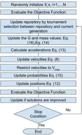
current generation and old repository and the new repository is updated as a result of this selection procedure. Tournaments selection is widely known to be an algorithm to preserve the diversity in the solutions. The flowchart of the proposed XOR BGSA with repository is depicted in Figure1, whereVmax refers to the maximum absolute value of velocity in each dimension.

Figure 1.Flowchart of the proposed XOR binary gravitational search algorithm (BGSA). 4. Theoretical Analysis of the Proposed XOR Binary Gravitational Algorithm with Repository 4.1. General Analysis of the Proposed XOR BGSA

The proposed XOR BGSA is investigated statistically to show that it is more compliant with the expectations of acceleration and velocity vectors of BGSA. Since the parameterXk(t), k=1, . . . ,Ncan only accept binary values ofzeroandone, the result of XOR operationXj(t)⊕Xi(t)may fall in each of the following categories.

(1) IfX_ik(t) =Xk_j(t) =0 orX_ik(t) =Xk_j(t) =1, in these casesXk_i (t)⊕Xk_j (t) =−1. It is expected from the acceleration term that since the corresponding bit in the best particle is the same as the bit in the current particle, the probability of change reduces. This expectation is fulfilled using (13).

(2) In the caseXk_j(t) =1, X_ik(t) =0,Xk_j(t)⊕Xk_i(t) =1, the acceleration term introduces a positive value which contributes positively to the probability of change and increases its value.

(3) In the case whenXk_j(t) =0, X_ik(t) =1,Xk_j(t)⊕X_ik(t) =1. Similar to the previous case, since the corresponding bit in the better particle is different than that of the current particle, a positive acceleration term is obtained which results in higher probability of change. This is an expected behaviour from the system.

According to this analysis, the issues mentioned earlier for BGSA do not exist in the proposed XOR BGSA.

4.2. Full Statistical Analysis of the Proposed Method

To perform theoretical analysis of the proposed XOR BGSA, a single dimensional optimization problem is considered. The parameterkbin this case is equal to1. Hence, in this section, we have a single particle whose behavior is studied and one best particle in the repository. The acceleration term, velocity term and the probability of change in the case of single dimensional optimization problem is obtained as follows:

a(t) =rjG(t) (Mrb(xrb(t)⊕x(t)))

kxrb(t)−x(t)krp+ε (18)

v(t+1) =piv(t)+a(t) (19)

P(v(t)) =0.5+0.5tanh(0.5v(t)) (20) wherea(t), v(t), P(v)are single dimensional vectors representing the acceleration, velocity and the probability of change corresponding to the studied particle. Furthermore,x(t)is the single dimensional vector representing the current position of studied particle andxrbis its corresponding value in the best particle in the whole population andMrbcorresponds to the mass of the best particle in the repository. The minimum value ofG(t)is equal toα1.

Two cases are investigated: the case whenpi=1 and the case when 0< pi<1 . Case I:pi=1

Lemma 1. If pi =1and x=xrb,∀t>0we have a(t)≤0and v(t+1)≤v(t).

Proof. Considering (13), we have the following equation for the acceleration terma(t):

a(t) =−r(t)G(t)MrbD≤0 (21)

where D = j1_εk is the dimension of the optimization algorithm. Consequently, considering (18), one obtains the following inequality:

v(t+1)=v(t)−r(t)G(t)MrbD≤v(t) (22)

This implies thatvtis monotonically non-increasing function of time.

Lemma 2. If pi =1and x(t) =xrbthen∀v,∃T>0s.t.∀t>Twe have E[v(t)]<v.

Proof. In the case when v(t0−1) < v, since according to Lemma 1 v(t) is monotonically non-increasing function of time, we have:

v(t0)≤v(t0−1)<v (23)

which means that∀t0<T Lemma2holds. However, in the case whenv≤v(t0−1), we have:

E[v(T)] =v(t0−1) +E " _T

∑

t−1 r(t)G(t)Mrb(xrb(t)⊕x(t)) kxb(t)−x(t)krp+1/D # (24) Sincex(t) =xrb, we have the following equation:

E[v(T)] =v(t0−1) +E " _T

∑

t−1 −r(t)G(t)MrbD # (25)

Considering the fact that minG(t) =α1, one obtains the following inequality: v(t0−1)−E " _T

∑

t−1 r(t)G(t)MrbD # ≤v(t0−1)−α1MrbD E " _T

∑

t0−1 r(t) #

To find the appropriateT, the following inequality needs to hold.

v(t0−1)−α1MrbD " _T

∑

t0−1 E[r(t)] # ≤v (26)

Considering the fact thatr(t)is a random variable uniformly distributed in [0, 1] , the following equation holds.

E[r(t)] =0.5 (27)

By applying expected value ofr(t)as in (27) to (26), the following equation is obtained.

v(t0−1)−0.5α1MrbD (T−t0+1)≤v (28) and finally T is obtained as follows:

2(v(t0−1)−v) Dα1

+t0−1≤T (29)

Since v(t−1) < v, ∀t0>1 from (29) we have 0≤T s.t. ∀t>T one obtains E[v(t)]<v. This concludes the proof.

Remark 1. Lemma2implies that in the case when the position in one dimensional optimization problem is the same as that of best particle, the velocity vector corresponding to that dimension grows in negative direction resulting in the probability of change to vanish to zero. This in turn results in no change in that dimension.

Lemma 3. If pi =1and x(t)6=xrb, then∀t>0, we have a(t)≥0and v(t+1)≥v(t). Considering (17), we have the following equation for the acceleration terma(t):

a(t) = r(t)G(t)Mrb

1+1/D ≥0 (30)

Consequently considering (30), one obtains the following inequality: v(t)≤v(t+1)=v(t) +r(t)G(t)Mrb

1+1/D (31)

This implies thatvtis monotonically non-decreasing function of time. Lemma 4. If pi =1and x(t)6=xrbthen∀v,∃T>0s.t.∀t>T, we have v<E[v(t)].

Proof. In the case when v<v(t0−1) since according to Lemma 3, v(t) is monotonically non-decreasing function of time we have:

v≤v(t0−1)<v(t0) (32)

which agrees with the Lemma4. However, in the case whenv(t0−1)≤v, we have:

E[v(T)] =v(t0−1) +E " _T

∑

t−1 r(t)G(t)Mrb(xrb(t)⊕x(t)) kxrb(t)−x(t)krp+1/D # (33)

Considering the fact thatx(t)6=xrb, the following equation is obtained. E[v(T)] =v(t0−1) +E " _T

∑

t−1 r(t)G(t)Mrb 1+1/D # (34) Considering the fact that minG(t) =α1, the following equation is obtained.

v(t0−1) +α1Mrb D 1+D E " _T

∑

t0−1 r(t) # ≤v(t0−1) +E " _T

∑

t−1 r(t)G(t)Mrb 1+1/D #

Hence, to findTwhich satisfies Lemma4, the following inequality needs to be hold.

v≤v(t0−1) +α1Mrb D 1+D " _T

∑

t0−1 E[r(t)] # (35)

Considering the fact thatr(t)is a random variable with uniform probability distribution function, the following equation holds.

E[r(t)] =0.5 (36)

By using the property ofr(t)as in (36), the following is obtained.

v≤v(t0−1) + 0.5α1D Mrb(T−t0+1)

1+D (37)

Hence, the value of T to satisfy Lemma 3 is obtained as follows: 2(1+D)e(v−v(t0−1))

Dα1Mrb

+t0−1≤T (38)

Since v(t0−1) < v, ∀t>1 from (38), we have 0 ≤ T s.t. ∀t>T and one has E[v(t)]< v. This concludes the proof.

Remark 2. It immediately follows from Lemma 4that in the case when the position in one dimensional optimization problem is different than that of the best particle, the velocity vector corresponding to that dimension grows resulting in the probability of change to increase to one which would result in increase in the probability of change.

Theorem 1. If pi=1.

1. In the case when x(t)=xrb, the acceleration term is non-positive and the velocity term is a non-increasing function of time and the probability of change converges to zero.

2. In the case whenx(t)6=xrb, the acceleration term is non-negative and the velocity vector is a non-decreasing function of time and the probability of change converges to zero.

Proof. Using Lemmas1–4, this theorem is concluded. Case II: 0< p_i<1:

Lemma 5. In the case when x(t) =xrb, ∀t>0 the velocity vector v(t)will never be larger than ptiv(0), where v(0)is the initial value of the velocity.

In the case when x(t) =xrb, from(17), it follows that

Considering(18), the following equation is obtained for v(t) v(t) =pt_iv(0)−D t

∑

τ=1 r(τ)G(τ)Mrb≤pitv(0) (40)

Hence, pt_iv(0)is an upper bound for v(t).

Remark 3. From Lemma5, it is concluded that in the case when x(t) =xrb, the acceleration term is non-positive acting in the direction of decreasing the probability of change. However, the impact of pt_iv(0)depends on the sign of v(0).

Lemma 6. In the case when x(t)6=xrb,∀t>0the velocity vector v(t)will never be smaller than ptiv(0). In the case when x(t)6=xrb, from(17), it follows that

a(t) =r(t)G(t)D Mrb≥0 (41)

Considering(18), the following equation is obtained for v(t)

pt_iv(0)≤v(t) =pt_iv(0) +D t

∑

τ=1

r(τ)G(τ)Mrb (42)

Hence, pt_iv(0)is a lower bound for v(t).

Remark 4. From Lemma 6, it is concluded that in the case when x(t)6=xb, the acceleration term is non-negative acting in favor of making probability of change in the corresponding bit higher. However, the impact of p_itv(0) depends on the sign of v(0).

Theorem 2. In XOR BGSA, considering sufficiently large number for maximum number of iterations, following properties hold.

1. Ifx(t) =xrb,∃T s.t.∀t>T, the probability of change becomes smaller than 0.5: P(x(t+1) =x(t))≤0.5

2. Ifx(t)6=xrb,∃T s.t.∀t>T, the probability of change becomes larger than 0.5: P(x(t+1) =x(t))≥0.5

In the case whenpi =1, from Theorem1it follows that whenx=xrb, as mentioned earlier in Remark1, the velocity value grows in negative direction which results in:

P(x(t+1) =x(t)) = 1

1+e−v(t) →0≤0.5 (43) Moreover, in the case whenpi=1, from Theorem1it follows that whenx(t)6=xrb, as mentioned earlier in Remark2, the velocity value grows larger which results in:

P(x(t+1) =x(t)) = 1

1+e−v(t) →1≥0.5 (44) Hence in the case of pi = 1, Theorem 2 holds. When 0 < pi < 1, two cases are considered. The case whenv(0) =0 andv(0)6=0.

Ifv0=0, in the case ofx=xrb, the velocity term according to (18) is obtained as follows: v(t) =−D t

∑

τ=1 r(τ)G(τ)Mrb≤0 (45) Hence: P(x(t+1) =x(t)) = 1 1+e−v(t) ≤0.5 (46)

In the case ofx(t)6=xrb, the velocity term according to (13) is obtained as follows:

v(t) =D t

∑

τ=1 r(τ)G(τ)Mrb≥0 (47) Hence: P(x(t+1) =x(t)) = 1 1+e−v(t)≥0.5 (48) Ifv(0)6=0, in the case ofx(t) =xrb, considering the fact that

v(t) =pt_iv(0)−D t

∑

τ=1

r(τ)G(τ)Mrb (49)

Ifv(0) < 0, from (49), it can be seen thatv(t)is the result of addition of two negative terms resulting in a negative value forv(t). However, ifv(0)>0, considering the factE[r(t)] =0.5, we have:

E[v(t) ] =pt_iv(0)−DE " _t

∑

τ=1 r(τ)G(τ) Mrb # ≤pt_iv(0)−α1.D MrbE "_T

∑

0 r(t) # =pt_iv(0)−0.5Tα1.MrbD (50)

Hence, the time T after which we haveE[v(t)]<0, is obtained from

pT_iv(0)−0.5Tα1.D Mrb<0 (51) and

2pT_i v(0)

α1D Mrb

<T. (52)

Hence, after a sufficiently large value of iterations specified by T,v(t)becomes negative and stays negative onwards. After that considering (19), we have the following:

P(x(T+1) =x(T)) = 1

1+e−v(T+1)≤0.5 (53) However, ifv(0)6=0, in the case ofx(t)6=xb, considering the fact that

v(t) =pt_iv(0) +D t

∑

τ=1

r(τ)G(τ)Mrb (54)

Ifv(0) > 0, from (54), it can be seen thatv(t)is the result of addition of two positive terms resulting in a positive value forv(t). However, ifv(0) < 0, similar to the analysis which resulted in (50) and considering the factE[r(t)] =0.5, we have:

E[v(t) ] =pt_iv(0)+DE " _t

∑

τ=1 r(τ)G(τ) Mrb # ≤pt_iv(0)+α1.D MrbE "_T

∑

0 r(t) # =pt_iv(0)+0.5Tα1.D Mrb (55)

Hence, the timeTafter which we havev(t)>0, is obtained from the following inequality pT_iv(0) +0.5Tα1.D Mrb>0 (56) and −2pT_i|v(0)| α1D Mrb <T. (57)

Hence after sufficiently large value of iterations specified byTin (57),v(t)becomes positive and stays positive on-wards. After that, considering the probability of change as in (19), it follows that:

P(x(T+1) =x(T)) = 1

1+e−v(t) ≥0.5 (58) This concludes the proof.

Remark 5. It immediately follows from Theorem2that if the value of a particle in one dimension is different than that of the best particle, the probability of change if not immediately, after sufficiently large number of iterations becomes larger than 0.5 making change in the corresponding dimension more probable than not. Moreover, if the value of particle in a dimension is similar to that of the best particle, the probability of change in that dimension if not immediately, after sufficiently large number of iterations becomes smaller than 0.5 making change in the corresponding dimension less probable.

Remark 6. The results obtained in Section4are valid for the case when kb =1. However, these results can be easily extended to the case when kb has a greater value in which case the value of kb particle effect other particles with a gain proportional to their mass. Hence, the overall probability of change is influenced by each of kbparticles disproportionately.

5. Simulation Results

5.1. Benchmark Optimization Problem

To evaluate the efficacy and performance of the proposed XOR BGSA with repository, it is tested against several benchmark problems. In optimization of benchmark problems, 20 bits are used to decode numerical values into the binary domain. The number of solutions considered (population size) is equal to 25, maximum number of generations are then selected to be equal to 1000. Two sets of comparisons are presented. In the first set of optimization, the proposed XOR BGSA is compared to BGSA [16], IBPSO [17], BPSO [15], BGWO [18] and BDA [19]. The main goal in these simulations is to demonstrate how the modifications proposed in this paper including the addition of XOR to the acceleration equation for BGSA as well as the repository effect its performance.

As in the real world, an optimization problem may be applied to a wide range of different functions including unimodal and multimodal problems, the proposed optimization algorithm is tested against both classes of optimization problems. The ability of the proposed optimization algorithm in dealing with problems with multiple local minimas is required to be investigated as well. For having such study, some of the optimization problems considered as the benchmark optimization problems include multiple local minimas. The benchmark problems considered are a collection of functions with single optimum solutions and functions with multiple local optimums. Other than these specifications, it is required to illustrate the performance of the proposed optimization algorithm in dealing with non-differentiable problems. The specifications of benchmark optimization problems are mentioned in front of them for ease of reference. The parameterNrepresents the dimension of these optimization problems which is considered to be equal to either 1, 2, 5 and 10 to test the optimization algorithms for different dimensions. These dimensions are multiplied by the number of bits taken for decoding real values, which results in optimization in 20, 40, 100 and 200 dimensional space. The mathematical formulas for the test functions as well as their specifications are as follows [20].

Sphere function[21]:a differentiable, separable, unimodal function without local minima f1(X) = N

∑

i=1 x2_i (59)

Multiplication of squares: a differentiable, non-separable, unimodal function without local minima

f2(X) =

∏

N_i=1ix2_i (60)

Griewark function[22]:a differentiable, non-separable, multimodal function with local minimas

f3(X) = 1 4000 N

∑

i=1 x2_i−

∏

N_i=1cos xi √ i (61) Schwefel function[23]:a differentiable, separable, multimodal function with local minima

f4(X) =− N

∑

i=1 xisin( q |xi|) (62)

Rastrigin Function[22]: a differentiable, separable, multimodal function with local minima

f5(X) =10.N+ N

∑

i=1 x2_i −10cos(2πxi) (63) Styblinski-Tang[24]:a differentiable, separable, multimodal function with local minima

f6(X) =1 N N

∑

i=1 x4i −16xi2+5xi (64) Michalewicz function[22]:a differentiable, separable, multimodal function with local minima

f7(X) =− N

∑

i=1 sin(xi) sin(ix2_i/π)20 (65)

Ackley function[25]:a differentiable, non-separable, multimodal function with local minima

f8(X) =−ae

−br 1 d∑30

i=1x2i _−e1d∑i=301cos(cxi)_+a+e1 ₍₆₆₎ Rotated hyperellipsoid function [22]: a differentiable, scalable, unimodal function without local minima f9(X) = N

∑

i=1 i

∑

j=1 x2j (67)

Alpine 1 function[22]:a non-differentiable, separable, multimodal function with local minima

f10(X) =

N

∑

i=1

|xisin(xi) +0.1xi| (68)

Cosine mixture function[22]:a differentiable, separable, multimodal function with local minima

f11(X) =−0.1 N

∑

i=1 cos(5πxi) − N

∑

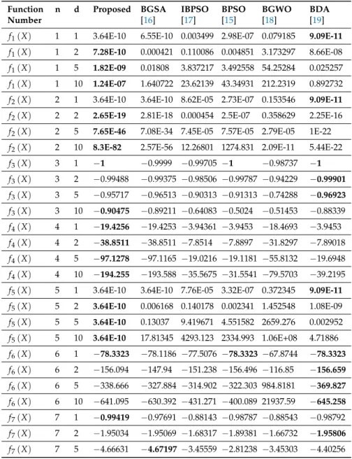
i=1 x2_i (69)

The results of comparison between the proposed algorithm and five other existing binary optimization algorithms are presented in Table2. Optimization process in each case is repeated for 30 times and the mean values are reported. It can be seen that the proposed optimization algorithm performs well in optimizing uni-modal as well as multi modal optimization problems. In 28 cases out of 44 cases, the proposed method outperforms other investigated optimization algorithms. It is further observed that when the proposed method is not the best optimization algorithm, it is still very close to the desired results. For instance, in the case of optimization function number 1, a uni-modal optimization problem, the proposed version of BGSA outperforms other algorithms in all different number of dimensions except for the case ofn= 1 where it is the second best optimization algorithm after BDA. Optimization function number 11, f11(x), is a multi-modal optimization problem with several local minimums for which the proposed XOR BGSA outperforms the other five investigated optimization algorithms in all four dimensions. It can further be observed from the Table2that BDA ranks the second after the proposed optimization algorithm.

Table 2.Optimization results using various optimization algorithms for the minimization of several benchmark optimization problems.

Function Number n d Proposed BGSA [16] IBPSO [17] BPSO [15] BGWO [18] BDA [19]

f1(X) 1 1 3.64E-10 6.55E-10 0.003499 2.98E-07 0.079185 9.09E-11

f1(X) 1 2 7.28E-10 0.000421 0.110086 0.004851 3.173297 8.66E-08

f1(X) 1 5 1.82E-09 0.01808 3.837217 3.492558 54.25284 0.025257

f1(X) 1 10 1.24E-07 1.640722 23.62139 43.34931 212.2319 0.892732

f2(X) 2 1 3.64E-10 3.64E-10 8.62E-05 2.73E-07 0.153546 9.09E-11

f2(X) 2 2 2.65E-19 2.81E-18 0.000454 2.5E-07 0.358629 2.25E-16

f2(X) 2 5 7.65E-46 7.08E-34 7.45E-05 7.57E-05 2.79E-05 1E-22

f2(X) 2 10 8.3E-82 2.57E-56 12.26801 1274.831 2.09E-11 5.44E-22

f3(X) 3 1 −1 −0.9999 −0.99705 −1 −0.98737 −1 f3(X) 3 2 −0.99488 −0.99375 −0.98506 −0.99787 −0.94229 −0.99901 f3(X) 3 5 −0.95717 −0.96513 −0.90313 −0.91313 −0.74288 −0.96923 f3(X) 3 10 −0.90475 −0.89211 −0.64083 −0.5024 −0.51453 −0.88339 f4(X) 4 1 −19.4256 −19.4253 −3.94361 −3.9453 −18.4693 −3.9453 f4(X) 4 2 −38.8511 −38.8511 −7.8514 −7.8897 −31.8297 −7.89018 f4(X) 4 5 −97.1278 −97.1165 −19.0216 −19.1181 −55.8132 −19.6948 f4(X) 4 10 −194.255 −193.588 −35.5675 −31.5541 −79.5703 −39.2195

f5(X) 5 1 3.64E-10 3.64E-10 7.76E-05 3.32E-07 0.372345 9.09E-11

f5(X) 5 2 3.64E-10 0.006168 0.140178 0.002341 1.452548 1.08E-09 f5(X) 5 5 3.64E-10 0.13037 9.419671 4.551582 2659.276 0.002952 f5(X) 5 10 3.64E-10 17.81345 4293.123 2334.993 1.06E+08 4.71886 f6(X) 6 1 −78.3323 −78.1186 −77.5076 −78.3323−67.8744 −78.3323 f6(X) 6 2 −156.094 −147.94 −151.238 −156.496 −116.85 −156.659 f6(X) 6 5 −338.666 −327.884 −314.902 −322.303 984.8181 −369.827 f6(X) 6 10 −641.095 −630.392 −431.271 −400.089 21937.59 −645.258 f7(X) 7 1 −0.99419 −0.97691 −0.88143 −0.98787 −0.88543 −0.98792 f7(X) 7 2 −1.95034 −1.95069 −1.68317 −1.89381 −1.66732 −1.95806 f7(X) 7 5 −4.66631 −4.67197−3.45559 −2.81238 −3.45303 −4.40256

Table 2.Cont. Function Number n d Proposed BGSA [16] IBPSO [17] BPSO [15] BGWO [18] BDA [19]

f1(X) 1 1 3.64E-10 6.55E-10 0.003499 2.98E-07 0.079185 9.09E-11

f7(X) 7 10 −8.83999 −9.00763−5.11393 −3.84276 −5.97745 −7.38148

f8(X) 8 1 7.63E-05 7.63E-05 0.17688 0.001563 1.270744 3.82E-05

f8(X) 8 2 7.63E-05 0.002378 0.873989 0.346521 3.054737 0.00026

f8(X) 8 5 7.63E-05 0.497182 4.210083 4.515039 9.078786 0.311861

f8(X) 8 10 0.07325 1.479706 6.721189 8.003571 11.92714 2.243791

f9(X) 9 1 3.64E-10 3.64E-10 0.000344 2.89E-07 0.052176 9.09E-11

f9(X) 9 2 1.09E-09 1.09E-09 0.285221 0.005263 3.989166 2.82E-08

f9(X) 9 5 5.46E-09 0.267058 10.71721 7.755365 108.3779 0.011655

f9(X) 9 10 3.09E-07 7.555599 125.9897 176.937 1128.728 5.058231

f10(X) 10 1 4.63E-06 2.32E-06 0.000547 2.03E-05 0.008308 2.88E-06

f10(X) 10 2 0.000948 0.000326 0.015704 0.003854 0.111948 0.000223 f10(X) 10 5 0.045093 0.021953 0.898418 1.041691 1.199264 0.080774 f10(X) 10 10 0.189655 0.304581 3.68566 6.668867 5.377988 0.748952 f11(X) 11 1 −400.1 −400.1 −99.9787 −100.093 −398.391 −100.1 f11(X) 11 2 −800.2 −799.77 −196.958 −198.57 −786.66 −200.195 f11(X) 11 5 −2000.5 −1996.02 −461.362 −442.035 −1900.74 −498.794 f11(X) 11 10 −4000.99 −3983.41 −839.887 −740.219 −3875.63 −974.665 5.2. Application to Knapsack

As the second class of benchmark optimization problem, the multi knapsack problem is considered. The problem formulation of 0/1 knapsack problem is discussed in summary in this part. Let there ben items with each having a positive profitpi >0 and a positive resource consumptionri >0. The main objective is to fill several knapsacks with resource capacity ofCjsuch that the accumulated profit of the items is maximized. Considering the constraints imposed by capacity of knapsacks, this problem is a constrained binary optimization problem. Such problems arises in various real-world applications such as in a distributed computer systems, warehouse optimization, cargo loading and stock problems [5,26]. This problem is explicitly formulated as follows:

f(x) =max n

∑

i=1 pixi (70) s.t. n

∑

i=1 rijxi≤Cj,j=1, . . . ,m (71) xi∈ {0, 1} ∀i∈{1, . . . ,n}

wherenrepresents the item number,mis the number of constrains,pi≥0 represents the profit value for each item, resource consumption is expressed byrij≥0 and the capacity is denoted by another positive valueCj≥0. The cost function is multiplied by negative value of−1 to change maximization to minimization problem. The constraints are added as penalty terms to the cost function to obtain an unconstrained optimization problem as follows:

fuc(x) =− n

∑

i=1 pixi+β n

∑

i=1 m

∑

j=1 min Cj−rijxi, 0 (72)

where the parameter β is used as the penalty coefficient and assigned the value equal to 1010. Several standard databases for knapsack optimization problems exist to provide means for comparison between the algorithms which provide special values forpi’s,Cj’s andrij’s. Among these database of multi knapsack optimization available at the website of Queen Mary University of London

(http://www.eecs.qmul.ac.uk/~jdrake/mkp.html) formerly hosted at University of Nottingham

(http://www.cs.nott.ac.uk/~jqd/mkp/index.html) are selected for performance comparison of the

proposed algorithms with several state-of-the-art binary optimization algorithms. The total number of populations are taken to be equal to 10 with maximum number of iterations selected to be equal to 1000.

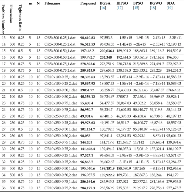
Table3presents the results obtained using the proposed optimization algorithm versus other optimization problems. The solutions are the optimization solutions to the function represented by (72) which are multiplied byminus oneto reflect the solutions to the original problem of (70) and (71). There exist several negative values in the table which show that in some cases, algorithms could not fulfil the constraints of optimization at least once. Such problem does not occur for the proposed XOR BGSA with repository. The best result obtained for each dimension is made bold faced to demonstrate its superior performance. The values used for optimization are collected from the website of Queen Mary University of London and their file names are presented for ease of reference. Problems have also been given a number for further discussions. As can be seen from Table3. The proposed XOR BGSA with repository outperforms all other investigated optimization problems in almost all cases.

The convergence property of the proposed approach versus previous optimization methods for optimizations number 7 to 12 are demonstrated in Figure2. As can be seen from this figure, the convergence of the proposed algorithm towards the solution is well above other investigated algorithms. Although during the first few iterations, some of the algorithms rise faster towards optimal solutions, after 100 iterations, the proposed XOR BGSA speeds up and becomes the dominant one. It can be concluded from the figure that other than quality of solutions, the speed of the proposed approach is well above other investigated optimization methods.

Table 3. Optimization results using various optimization algorithms for the maximization of the knapsack problem. Problem Number Dimension T ightness Ratio

m N Filename Proposed BGSA

[16] IBPSO [17] BPSO [15] BGWO [18] BDA [19]

1 100 0.25 5 10 OR5x100-0.25 1.dat 21675.33 20,742.73 −7E+13 −1.4E+14−3.6E+14 20,278.77 2 100 0.25 5 10 OR5x100-0.25 2.dat 21,223.93 20,663 −9.2E+13−1.4E+14−3.4E+14 19,938.63 3 100 0.5 5 10 OR5x100-0.50 1.dat 39,835.93 39,302.37 37,097.47 37,573.93 37,093.93 38,813.2 4 100 0.5 5 10 OR5x100-0.50 2.dat 39,812.4 39,372.73 36,388.13 37,300.47 36,902.1 38,704.93 5 100 0.75 5 10 OR5x100-0.75 1.dat 57,626 56,945.5 52,385.83 50,954.87 55,652.37 56,107.47 6 100 0.75 5 10 OR5x100-0.75 2.dat 59,946.2 59,272.1 55,457.23 53,529.87 57,861.93 58,294.9 7 250 0.25 5 10 OR5x250-0.25 1.dat 49,323.17 46,860.27 −5.9E+14−7.6E+14−1.1E+15 46,805.43 8 250 0.25 5 10 OR5x250-0.25 2.dat 51,256.37 49,071.9 −6.1E+14−7.7E+14−1.2E+15 48,596.37 9 250 0.5 5 10 OR5x250-0.50 1.dat 99,682.27 99,393.17 94,943.5 94,993.6 94,801.07 97,535.43 10 250 0.5 5 10 OR5x250-0.50 2.dat 99,759 99,000.57 94,482.33 94,256.9 94,158.23 97621.53 11 250 0.75 5 10 OR5x250-0.75 1.dat 142,598.2 140,975.2 120,843.3 115,794.4 139,086.3 139,172.7 12 250 0.75 5 10 OR5x250-0.75 2.dat 147,544.4 145,975.8 124,749.9 119,751.7 143,700.6 144207.3

Table 3.Cont. Problem Number Dimension T ightness Ratio

m N Filename Proposed BGSA

[16] IBPSO [17] BPSO [15] BGWO [18] BDA [19]

13 500 0.25 5 15 OR5x500-0.25 1.dat 98,610.83 97,553.3 −1.5E+15−1.9E+15−2.4E+15−3.2E+11 14 500 0.25 5 15 OR5x500-0.25 2.dat 96,512.53 96,034.53 −1.4E+15−2E+15 −2.5E+15 92,190.13 15 500 0.5 5 15 OR5x500-0.50 1.dat 197448.2 200,036.1 189,901.2 188,863.1 189,116.2 194,592.8 16 500 0.5 5 15 OR5x500-0.50 2.dat 199,792.7 202,340 192,444.5 190,561.9 191,162.6 196,350 17 500 0.75 5 15 OR5x500-0.75 1.dat 278,893.6 278,751.9 228,713.8 215,389.8 274,491.7 272,973.2 18 500 0.75 5 15 OR5x500-0.75 2.dat 289,925.9 289,654.3 238,158.3 223,533.2 285,228 284,254.3 19 100 0.25 10 10 OR10x100-0.25 1.dat 20,393.63 18,793.87 −1.8E+14−2.9E+14−7.4E+14 18,583.23 20 100 0.25 10 10 OR10x100-0.25 2.dat 19,867.93 18,857.43 −1.8E+14−2.6E+14−7.1E+14 18,583.03 21 100 0.5 10 10 OR10x100-0.50 1.dat 39051.77 38,258.77 35,430.33 36,021.43 35,607.37 37669.33 22 100 0.5 10 10 OR10x100-0.50 2.dat 40,356.13 39,734.97 37007.3 37,450.4 36,969.97 38,926.1 23 100 0.75 10 10 OR10x100-0.75 1.dat 55,408.4 54,477.57 50,067.83 49,302.2 53,058.4 53,580.87 24 100 0.75 10 10 OR10x100-0.75 2.dat 56,950.7 56,234.7 51,602.53 50,940.77 54,119.3 55,144.23 25 250 0.25 10 10 OR10x250-0.25 1.dat 49,901.6 49,401.6 46,393.33 46,438.4 46,738.6 48,197.13 26 250 0.25 10 10 OR10x250-0.25 2.dat 49,978.63 49,191.07 46,514.7 46,100.77 46,874.6 48,557.03 27 250 0.5 10 10 OR10x250-0.50 1.dat 101,134.7 100,792.5 96,179.27 95,810.07 −4.8E+11 99,126.03 28 250 0.5 10 10 OR10x250-0.50 2.dat 98,053 97,841.1 92,281.53 92,293.1 −8.8E+11 95,604.23 29 250 0.75 10 10 OR10x250-0.75 1.dat 144,205 141,717.6 121,695.7 117142 139,645.4 139,894.6 30 250 0.75 10 10 OR10x250-0.75 2.dat 141,698.4 139,494.2 120,037.3 115,081.9 137,321.4 138,109.7 31 500 0.25 10 15 OR10x500-0.25 1.dat 97,327.1 96,654.03 −2.9E+15−3.9E+15−4.9E+15 93,571.07 32 500 0.25 10 15 OR10x500-0.25 2.dat 96,865.7 96,662.67 −3.1E+15−4.1E+15−5.1E+15 93,284.37 33 500 0.5 10 15 OR10x500-0.50 1.dat 195,540.6 199,151.9 188,580.9 187,265 −8.1E+11 192,963.6 34 500 0.5 10 15 OR10x500-0.50 2.dat 196,987.5 199,922.2 189,706.1 187,867.3 188,244 194,179 35 500 0.75 10 15 OR10x500-0.75 1.dat 286,164.6 285,945.3 237,022 220,772.4 281,163.6 279,953.5 36 500 0.75 10 15 OR10x500-0.75 2.dat 284,177.3 283,569.9 235,502.1 219,917.2 278,756.1 277,475.7

In most real-world optimization problems, the cost function evaluation requires high volume of computation. Hence, it would be highly desired for an optimization algorithm to result in superior performance after its single run. Box plot is a graphical method which gives more information about the diversity of the results rather than just its mean value. A small standard deviation leads to a smaller interquartile range which can be interpreted as its ability to avoid local minima. Outliers can also be easily spotted from box plot. In Figure3while the interquartile is illustrated using a blue box, the minimum and the maximum associated with data are demonstrated using the black line. There is a 50 percent chance that for a new experience, the result falls within the interquartile range. The outliers in this figure are represented by “+” sign. The median values are demonstrated with red line. The box plot obtained using different optimization algorithms for optimization problems 7 to 18 are illustrated. It can be observed from the figure that not only the median values obtained for the proposed approach in 10 cases out of 12 cases are the best, interquartile range obtained for the proposed approach in most cases is smaller meaning that it is more repeatable than in other investigated optimization algorithms. Furthermore, for optimization problems numbers 7, 8, 11 and 12, it can be observed that the interquartile range obtained for the proposed approach is well above the other optimization algorithms. This means that for every single run of the proposed optimization algorithm, there is

an appreciable chance we can obtain superior performance for the proposed optimization algorithm compared to other investigated optimization methods.

(a) Problem #7 zz (b) Problem #8 zz (c) Problem #9 zz (d) Problem #10 zz (e) Problem #11 zz (f) Problem #12 zz

Figure 2. Trend of Cost function obtained from proposed XOR BGSA vs. four other algorithms namely: BGSA [16], improved binary particle swarm optimization (IBPSO) [17], binary particle swarm optimization (BPSO) [15], binary grey wolf optimization (BGWO) [18] and binary dragonfly optimization algorithm (BDA) [19]. Knapsack optimization problems numbers 7 to 12.

(a) Problem #7 zz (b) Problem #8 zz (c) Problem #9 zz (d) Problem #10 zz (e) Problem #11 zz (f) Problem #12 zz (g) Problem #13 zz (h) Problem #14 zz (i) Problem #15 zz (j) Problem #16 zz (k) Problem #17 zz (l) Problem #18 zz

Figure 3.Box plot obtained for the knapsack problem using the proposed XOR BGSA vs. three other algorithms namely: BGSA [16], BGWO [18] and BDA [19]. Knapsack optimization problems 7 to 18. 6. Industry 4.0 Applications

In current manufacturing environments, modifications made to a product often require redesign and retraining/programming of production elements on the factory floor. Optimal or sub-optimal solutions to design changes in a process is the goal of decision-making processes. Recent work has explored showing that systematic optimization is possible in a well-defined detailed digital twin in which searching algorithms can perform multiple trial and errors without safety and resource restrictions. Additionally, current robot programming techniques require highly talented professionals

to perform programming, which increases response times and increases costs [27]. Real-time decision making and robot programming is therefore highly desirable and is a stated requirement of Industry 4.0 [28]. However, autonomous programming of robots will impact safety and certification requirements as well. To mediate such impacts, one solution is to tie the digital twin solutions to the real-production methods. Such a digital twin needs to be as accurate as possible to ensure compatibility of actions with real world. The simulated movements in such an environment can then be transformed to the real robot after full examination of resulting optimization solutions by a human expert. This framework makes the most of machine learning and artificial intelligence approaches. In this part, the proposed XOR BGSA with repository is used to find an optimal solution for assembly task planning and motion planning for an industrial robot namely UR5 that would then be passed to a human for certification before implementation. Previously the proposed XOR BGSA is tested against different types of optimization problems including uni-modal, multi-modal, those with single optimum solution, those which suffer from multiple local minimums and knapsack optimization problem which is a constrained one. The fact that the proposed optimization procedure obtained the best results among six binary optimization problems in most cases motivates us to use it in Industry 4.0 optimization problems.

It is required for robots to be able to optimally plan their own task autonomously otherwise massive resources may be used to redesign, reconfigure and reprogram them. To fulfil this goal, it is required to decode the planning process in the form of an optimization problem and use artificial intelligence approaches to solve the problem on a UR5 capable of handling 5 Kg loads to a precision of order of 0.1 mm .

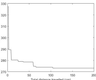
The assembly task planning to be optimized in this application is to put bolts in their respective places while minimizing the distance. The bolts used in this study are from three different types of ofM6×20 mm,M8×20 mm and M10×20 mm. Hence, we have three different type of nuts which must be fastened using the bolts. The place and the position of the nuts and bolts are depicted in Figure4with thezcomponent of position for nuts being on 5.7 cm and for bolts being equal to 7 cm. Such an assembly task is similar to the benchmark problem frequently solved in computer science projects called the travelling salesperson. The cost function to be optimized in this case is the total distance travelled with main difference between the assembly task designed to test the proposed XOR BGSA and the travel salesperson being that in the current experiment, we have certain bolts which can be used to fasten certain nuts; this imposes some constrains on the optimization problem.

To encode the optimization problem, 31 bits are considered for each individual. Inspired by the results obtained by the proposed optimization procedure, it is used to minimize the total distance travelled by UR5 during the assembly task of industrial calculator (See Figure5). In this case, there exist 231 =2.1475×109 different combinations for performing the assembly task. As can be seen from Figure5, the first two bits determine which bolts are used to fasten nut #1, the bits numbers 3 and 4 are used to determine which bolts are used for nuts number 2, the fifth bit is for nut number 3. Since we have fourM10×20 mm bolts, the remaining bolt goes to nut number 4. Bit number 6 determines whichM8×20 mm is used to fasten nut number 5, the other one is used to fasten bolt number 6. The bit number 7 is used for bolts numbers 7 and 8. However, since the order of performing these tasks effects the cost function, it is required to determine the order of performing the tasks using the next 24 bits. All 3 of them making an integer value from the interval of[0, 7]. In this case, if theith value after converting to decimal value is equal toj, theith andjth task swap their position. This results in avoiding forbidden conditions which is difficult to avoid otherwise. The cost function to be optimized is the total distance travelled by robot with its initial conditions being at point(10, 30, 10).

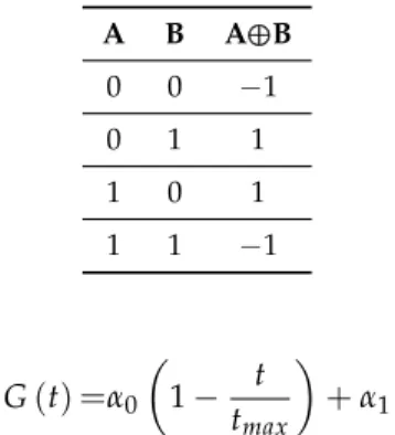
The evolution of total distance travelled by the robot is depicted in Figure6. The total number of particles in this optimization is chosen to be 10 with the maximum number of iterations being equal to 200. As can be seen from this figure, the best random initialization for the total distance travelled by robot is 328.0 cm which decreases to 273.2 cm after optimization, resulting in a 16.7% improvement. The optimum solution of the problem is represented in Table4and the assembly process done by

UR5 is illustrated in Figure7. The total assembly time is 116 seconds. Where for our laboratory safety reasons, the joint speed of the robot is limited to 90/s. However, as the UR5 is capable of working with joint speed equal to 180/s, the total assembly time could be reduced if it works under full speed.

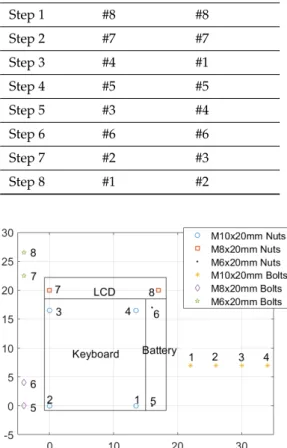
Table 4.Optimal assembly solution obtained from the optimization algorithm.

Action Bolt Nut

Step 1 #8 #8 Step 2 #7 #7 Step 3 #4 #1 Step 4 #5 #5 Step 5 #3 #4 Step 6 #6 #6 Step 7 #2 #3 Step 8 #1 #2

Figure 4.2D position of nuts and bolts in assembly task.

Figure 6.Evolution of total distance travelled by UR5 versus iterations.

Figure 7.Movements obtained from optimization.

6.1. Motion Planning of Industrial Robots Inside a Digital Twin Created by V-REP Software

Proposed XOR BGSA with repository is used to find the optimal path for an industrial robot in its digital twin environment. The industrial robot used in this part is of a cobot type namely UR5. Cobot is a slang which refers to collaborative robot, generally accepted as any robot designed to operate in close proximity to human workers without need for a separating cage. The problem considered here is to find the shortest collision free path for the robot in 3D space while undergoing a pick and place task. Figure7illustrates the digital twin of the manufacturing environment simulated in V-REP software, where there exist a human worker working closely to the robot.

Simulations have been carried out using V-REP software, a user-friendly software, which works under various operating systems including Windows. This software V-REP is designed around a versatile architecture with different independently working functions. The options embedded in this

software can be easily enabled or disabled as required. The communication with this software is possible from ROS using rostopics as well as directly from Python or Matlab using respective API developed specially for this software. A wide range of robots including industrial robots from different companies including Universal Robots are available in this software. The driver included in this software for each of these robots possesses much of real robot features including stopping movement in the case of collision with an object. Real features of robot including maximum speed, maximum joint angles and maximum torque are available in the robot and may be modified at user desire making it replicate the real robot as much as possible. Another feature which exist under V-REP software is its ability to compute the inverse kinematic of robot and find the joint angles of the robot automatically which considerably facilitates robotic simulation.

The obstacles in this environment are possible obstacles in real manufacturing environments such as other machines, tools and devices. V-REP software is a robust software for simulating the physical behaviours of objects, including collision between them as well as forces such as gravity and friction that can all be included as part of the software environment. In this way, the user can easily define object positions and orientations while the V-REP software takes care of updating movement of the various other objects and collisions which may happen during motion. As the result is a game like 3D interface, examination of the movement can be easily achieved by the human expert. In this way the human expert can ascertain if there may be problems with the solution that are not specified in the programming. To perform the automated optimization, it is required that the robot movements be encoded in terms of an evolvable array which may then be translated to motions to evaluate cost function and make changes to optimize the problem. A similar approach has been previously done using Ant colony optimization in another software namely Gazebo [28]. However, the benefit of using V-REP versus Gazebo is that the former benefits from built-in inverse kinematic which makes it possible to perform the simulations in a timely manner. A comparative study has been performed previously in [29] which compared V-REP software and Gazebo. It is concluded that V-REP is a more user-friendly and intuitive software than Gazebo in which intelligent optimization can be carried out with more comfort.

While Figure8depicts the real robot, its digital twin developed in V-REP is depicted in Figure9. As can be seen from these figures, digital twin matches with real robot in terms of dimensions and position of robot and obstacles, respectively. As can be seen from this figure, several objects as well as the UR5 robot exist in this digital twin. The obstacles are in the form of several cubic boxes which replicate the machines and devices which exist close to the robot.

Figure 9.Digital twin of manufacturing environment developed in V-REP. 6.1.1. Encoding Movements

To optimize movements, they are encoded in terms of an evolvable array according to the proposed XOR BGSA with repository which is implemented under Matlab software. In this paper, it is assumed that the initial orientation of the robot remains the same during optimization and its position needs to be changed to perform the displacement from the start point to the end point. Considering three x, y and z dimensions and the fact that they can be increased and decreased, there would be six movements which can be represented by any integer value from the setS = {0, 1, . . . , 5}. However, the proposed optimization algorithm would generate three bits for each movement. To avoid infeasible solutions, the set is considered to have all eight conditions and duplicate movements may be added. Moreover, during optimization duplicate coordinates may occur as a result of back and forth in the movements. To avoid such loops in robot movement, all coordinates are compared with each other and all intermediate movements which result in a loop are eliminated. The interpretation of movements are presented in Table5.

Table 5.Interpretation of values of array generated by the proposed XOR BGSA.

Movements Rotations

Value Interpretation Value Interpretation

0 x=x+0.025 4 z=z+0.025

1 x=x−0.025 5 z=z−0.025

2 y=y+0.025 6 x=x+0.025

3 y=y−0.025 7 x=x−0.025

6.1.2. Kinematic and Inverse Kinematic of UR5

The UR5 robot benefits from 6-degrees of freedom. Position and orientation of this robot and its end-effector in 3D work-space is represented byx∈R6. While the first three dimensions of this vector present three translational variables, the next three dimensions represent its orientation. The joint angles, represented by q = h q1 q2 . . . q6 i, are solutions to the inverse kinematic problem.

The forward kinematic function is the function used to compute the position and orientation of the robot corresponding to its assigned joint angles.

x=F K(q) (73)

The standard Denavit–Hartenberg (DH) convention to represent the forward kinematics of the robot is used in this paper. The DH parameters associated with UR5 are presented in Table6. Using such convention, inverse kinematic of the robot can be found as follows:

x=T₁0T₂1T₃2T₄3T₅4T₆5 (74) whereT_ii−1presents the homogeneous transformation matrix which makes the transform from frame i−1 to frameidefined as follows:

T_ii−1=      c(qi) −s(qi)c(αi) s(qi)s(αi) ric(qi) s(qi) c(qi)c(αi) −c(qi)s(αi) ris(qi) 0 s(αi) c(αi) di 0 0 0 1      (75)

wheres(.) andc(.) represent the sinus and cosine of their arguments. The values obtained from the movement array need to be translated in terms of robot movements. To enable this a transformation matrix that represents position and orientation of robot is obtained based on work by [30,31]. The transformation matrix for frame 6 with respect to frame 0 is as follows:

6 0T(θ1,θ2,θ3,θ4,θ5,θ6) = " 0 6R 06P 0 1 # =      0 6Xˆx 06Yˆx 06Zˆx 06Px 0 6Xˆy 06Yˆy 06Zˆy 06Py 0 6Xˆz 06Yˆz 06Zˆz 06Pz 0 0 0 1      (76) where0

6Xˆ,06Yˆ and06Zˆ are unit vectors defining the axis of frame 6 in relation to frame 0 and: 0

6R=Rx(a)Ry(b)Rz(c) in which the rotational matrices are obtained as follows:

Rx=    1 0 0 0 cosa −sina 0 sina cosa    (77) Ry=    cosb 0 sinb 0 1 0 −sinb 0 cosb    (78) Rz=    cosc −sinc 0 sinc cosc 0 0 0 1    (79)

Inverse kinematics are then used to find joint angles of robot to move to a desired position given by proposed XOR BGSA. The angles of the robot are then obtained as [30,31]:

θ1 = atan2 0 5yP,05xP +acos   d4 q 0 5xP2+05yP2  + π 2 θ2 = atan2 −1_4zP,−1_4xP−asin −a3sinθ3 |1 4xzP| ! θ3 = ±acos |1 4xzP| 2 −a22−a32 2a2a3 ! θ4 = atan2 3 4yXˆ ,34xXˆ θ5 = ±acos 0 6xPsinθ1 − 06yPcosθ1 −d4 d6 ! θ6 = atan2(M1, M2) where: M1=− 6 0yXsinˆ θ1 +60yYcosˆ θ1 sinθ5 (80) M2= 6 0yXsinˆ θ1 −60yYcosˆ θ1 sinθ5 (81)

Table 6.Denavit–Hartenberg (DH) parameters representing the forward kinematics.

i di(mm) θ ai(mm) αi(rad) 0 – – 0 0 1 89.16 q1 0 π 2 2 0 q2 −425 0 3 0 q3 −392.25 0 4 109.15 q4 0 π2 5 94.65 q5 0 −π2 6 82.3 q6 0 0

6.1.3. Communication between Matlab and V-REP

Communication between Matlab and V-REP is done using API developed by Coppelia robotics. Figure10demonstrates the overall communication requirement between Matlab and V-REP. As can be seen from this figure, proposed XOR BGSA with repository generates the path in terms of a binary sequence. This binary sequence is then translated to real movement with required resolution. Such movements are transmitted to V-REP in terms of positions and orientations of robot which is translated to joint angles of robot using built in inverse kinematic software. When a collision occurs, the target position of robot needs to be modified to the last possible point before collision in the system. After performing simulation, the results including total simulation time and distances are reported back as the real-world perception of the binary code in terms of a cost function. After all particles are evaluated, the proposed XOR BGSA iterates for another iteration to generate the next solutions.

The parametersxi,yi,zi,ai,biandciare the position and orientation of robot after every movement. Since obstacles are static objects in V-REP, in case of a collision, the robot stops, and a collision flag is returned. Furthermore, the desired position given to the robot is not met because of collision. Hence,

the difference between desired and obtained position of robot is a measure of collision. Such position difference can be used to penalize the cost function. The increment in the position suggested by the proposed XOR BGSA would be the actual position of robot plus the decoded increment from Table5.

Figure 10.Communication between Matlab and V-REP. 6.1.4. Cost Function to Be Optimized

As the goal of the optimization is to obtain a desired position and orientation while ensuring that no collision happens, total distance between the desired position and the actual position of the robot is as follows:

DT=

∑

i

(xi−xd)2+(yi−yd)2+(zi−zd)2 (82)

wherexd, ydand zdare coordinates ofPDthe desired position of the robot. Other than distance to the desired position, total time is used as another term in the cost function.

f(x) =KDDT+KTT+DC (83)

whereTrepresents the total time,DCrepresents the distance between the actual position of robot and its desired position in every single movement due to collision with obstacles. The parametersKDand KTare two gains used for optimization which are selected as equal to 10,000 and 1, respectively.

For each individual particle, after performing the movements given by the particle,PDis given as the final position of the robot. Meanwhile if there exist no obstacles between the last position obtained from the proposed optimization algorithm andPD, robot moves easily to the final position. Otherwise, obstacle stops robot from movement. It is further assumed that if the end effector is close to the desired point robot does not need to continue with the movements given by the proposed XOR BGSA and total time is considered to this point. When end effector is within obstacle free range of the desired position, the other movements given by the proposed XOR BGSA are bypassed and the desired position is used as the next step for robot.

6.1.5. Simulation Results

The proposed XOR BGSA with repository is iterated for 30 times in Matlab software connected to V-REP through API using 30 particles. The evolution of cost function during optimization is depicted in Figure11on a logarithmic scale. As can be seen from this figure, the best cost function value among the 30 particles starts from a high value of 3446 due to collisions and is reduced during optimization to 6.77, which is a collision free, time optimal solution to the problem which hits the desired point. This indicates that for the final collision free solution, the total time is equal to 6.77 s.

Figure 11.Cost function values associated with UR5 during path planning application.

The resulting movements are depicted with a red line in Figure12, which can be inspected by human expert before final implementation on a real robot.

The 3D environment provided by simulation software provides complete visual demonstration of movements, which makes it is easy to perform the inspection and ensure suitability of the solution to real-world implementation before that happens. This can be an important safety feature within any working environment and such linking between the human and automated elements of production is a key factor in Industry 4.0 practice.