C A R F W o r k i n g P a p e r
CARF-F-002
Empirical Likelihood Estimation of Levy Processes
Naoto Kunitomo University of Tokyo Takashi Owada Bank of Japan April 2004 Revised: March 2005
CARF is presently supported by Bank of Tokyo-Mitsubishi UFJ, Ltd., Dai-ichi Mutual Life Insurance Company, Meiji Yasuda Life Insurance Company, Mizuho Financial Group, Inc., Nippon Life Insurance Company, Nomura Holdings, Inc. and Sumitomo Mitsui Banking Corporation (in alphabetical order). This financial support enables us to issue CARF Working Papers.
CARF Working Papers can be downloaded without charge from: http://www.carf.e.u-tokyo.ac.jp/workingpaper/index.cgi
Working Papers are a series of manuscripts in their draft form. They are not intended for circulation or distribution except as indicated by the author. For that reason Working Papers may not be reproduced or distributed without the written consent of the author.
Empirical Likelihood Estimation of L´
evy Processes
∗ Naoto Kunitomo†and
Takashi Owada ‡ May 2004 (1st Version) February 2005 (Revised Version)
Abstract
We propose a new parameter estimation procedure for the L´evy processes and the class of infinitely divisible distribution. We shall show that the empirical like-lihood method gives an easy way to estimate the key parameters of the infinitely divisible distributions including the class of stable distributions as a special case. The maximum empirical likelihood estimator by using the empirical characteristic functions gives the consistency, the asymptotic normality, and the asymptotic ef-ficiency for the key parameters when the number of restrictions on the empirical characteristic functions is large. Test procedures can be also developed. Some extensions to the estimating equations problem with the infinitely divisible distri-butions are discussed.
Key Words
Stable Distribution, L´evy processes, Infinitely Divisible Distributions, Maximum Em-pirical Likelihood, Characteristic Function, Estimating Equation Methods.
AMS Subject Classification: Primary 60G51, 60G52; secondary 62F12.
∗This paper is a revised version of Discussion Paper CIRJE-F-272 (2004), Graduate School of
Economics, University of Tokyo. We thank Professor Y. Miyahara of Nagoya-City University, the associate editor and the referee of this journal for pointing out several problems contained in the original paper which have led us to revise it significantly.
†Graduate School of Economics, University of Tokyo, 7-3-1 Hongo, Bunkyo-ku, Tokyo 113-0033,
JAPAN.
1. Introduction
There have been growing interests on the applications of the L´evy processes and the class of infinitely divisible distributions in several research fields including financial economics. One interesting class of infinitely divisible distributions is the class of stable distributions. Since they are important classes of probability distributions, there have been extensive studies by mathematicians in probability over several decades. See Feller (1971), Zolotarev (1986), and Sato (1999) for the details of related problems in the probability literatures. Several statistical applications of stable distributions have been applied for modeling the fat-tail phenomena sometimes observed in financial economics and other applied areas of statistics. See Mandelbrot (1963), Paulson et. al. (1975), and Nolan (2001) for the early studies of the subject in the statistics literatures. More recently, some applications of the more general L´evy processes and other class of infinitely divisible distributions have been reported in the analyses of financial data. See Bandorff-Nielsen et. al. (2001) and Carr et. al. (2002) for recent examples.
Several estimation methods for the key parameters of stable distributions have been proposed and developed over the past few decades. DuMouchel (1971) has investigated the parametric maximum likelihood estimation method and Nolan (1997) has extended a numerical algorithm of the likelihood evaluation. Since it is not possible to obtain any explicit form of the likelihood function for stable distributions except very special cases, Fama and Roll (1968, 1971) proposed a practical estimation method based on the percentiles of empirical distributions and later MuCulloch (1986) has improved their method. Also another estimation method based on the empirical characteristic function was originally proposed by Press (1972), and there have been several related studies by Paulson et. al. (1975), Koutrouvelis (1980), Kogon and Williams (1998), Feuerverger and McDunnough (1981a, 1981b). These estimation methods could be extended to the more general L´evy processes.
The main purpose of this paper is to develop a new parameter estimation procedure for the L´evy processes and some classes of infinitely divisible distributions based on the empirical likelihood approach. The empirical likelihood method was originally proposed by Owen (1988, 1990) for constructing nonparametric confidence intervals and later it has been extended to the estimating equations problem by Qin and Lawless (1994). In this paper first we shall show that we can apply the empirical likelihood approach to the estimation problem of unknown parameters for stable distributions and the resulting computational burden is not heavy. In particular, the maximum empirical likelihood (MEL) estimator for the parameters of stable distribution we are proposing has some desirable asymptotic properties; it has the consistency, the asymptotic normality, and the asymptotic efficiency when the number of restrictions on the empirical characteristic function is large under a set of general conditions. Also it is possible to develop the empirical likelihood ratio statistics for the parameters of stable distributions which have the desirable asymptotic property.
More importantly, it is rather straightforward to extend our estimation method for the unknown parameters of stable distributions to the estimation of L´evy processes and infinitely divisible distributions, and also to the estimating equations problem with stable disturbances and other infinitely divisible disturbances. We shall show that it is possible to estimate both the parameters of equations and the parameters of stable distributions (or some infinitely divisible distributions) for disturbances at the same
time by our method. It seems that it is not easy to solve this estimation problem by the conventional methods proposed in the past studies and in this sense our estimation method has some advantage over other methods. For the estimating equations problem, Qin and Lawless (1994) have shown some asymptotic properties of the MEL estimator and Kitamura et. al. (2001) have extended their results to one direction. In this respect our study has some technical novelty because we are considering the case when the number of restrictions grows with the sample size. Hence this paper can be regarded as an extension of Qin and Lawless (1994) in another important direction. Our formulation of the empirical likelihood method with many restrictions is closely related to a recent unpublished work by Hjort et. al. (2004). Also the studies by Fan et. al. (2001), Shen et. al. (1999), and Zhang and Gibels (2003) on the hypotheses testing problems have discussed the related problems.
In Section 2, we formulate the empirical likelihood estimation method of the class of stable distributions in the standard situation and state our main results on the asymptotic properties of the MEL estimator and the related testing procedure. Then in Section 3, we discuss the estimation problem of the L´evy processes and several infinitely divisible distributions, and an extension to the estimating equations problem when the disturbance terms follow the stable distribution (or some infinitely divisible distributions). In Section 4, we report some simulation results and in Section 5 we give some concluding remarks. The proofs of main results are given in Mathematical Appendix.
2. Empirical Likelihood Estimation of Stable Distributions
In this section we first consider the situation whenXi (i= 1, . . ., n) are a sequence
of independently and identically distributed random variables and they follow the class of stable distributions. Let the characteristic function ofXibe denoted byφθ(t),and its real part and imaginary part beφRθ(t) andφIθ(t),respectively. We adopt the formulation of the characteristic function used by Chamber et. al. (1976) for the class of stable distribution and it is represented as
(2.1) φθ(t) =φθR(t) +iφIθ(t),
where
φRθ(t) = e−|γt|αcos[δt+βγt(|γt|α−1−1) tanπα2 ] , φIθ(t) = e−|γt|αsin[δt+βγt(|γt|α−1−1) tanπα2 ] and the parameter space is given by
Θ={0< α≤2,−1≤β≤1, γ >0, δ∈R}.
In the following analysis we denote the vector of unknown parametersθ = (α, β, γ, δ) and the stable distribution associated with θ asFθ(·).
There are two non-standard problems in the estimation of the vector of unknown parameters θ. It has been well-known in probability theory that except some special cases (the normal distribution, the Cauchy distribution, and a L´evy distribution) we do not have a simple explicit form of the probability density function and distribution function. This makes some difficulty of the direct estimation of unknown parameters including the parametric maximum likelihood method. Also since the stable distribu-tions do not necessarily have the first and/or second moments, some of the standard techniques in the statistical asymptotic theory cannot be directly applicable.
2.1 Empirical Likelihood Method
In order to estimate the unknown parameters of the stable distributions, we are propos-ing to use the empirical likelihood approach, which is similar to the one developed by Qin and Lawless (1994). Because the stable distributions do not necessarily have the first and second moments, we cannot utilize the moments of distributions. However, we can use the information from the empirical characteristic functions instead. We define the empirical likelihood function by
(2.2) Ln(Fθ) = n k=1 (Fθ(Xk)−Fθ(Xk−)) = n k=1 pk,
where Fθ(·) is the distribution function and pk (k = 1,· · ·, n) are the probability as-signed to the data points of Xk. Without any further restrictions except pk ≥ 0
and nk=1pk = 1, the empirical likelihood function Ln(Fθ) can be maximized at
pk= 1/n(k= 1,· · ·, n). Let the empirical likelihood ratio function be (2.3) Rn(Fθ) =
n
k=1
npk.
Then we define the maximum empirical likelihood estimator ˆθn for the vector of
un-known coefficients by maximizing the functionRn(Fθ) under the restrictions
Pn= pk≥0 (k= 1, . . ., n), n k=1 pk= 1, n k=1 pk cos(tlXk)−φRθ(tl) = 0, n k=1 pk sin(tlXk)−φIθ(tl) = 0 (l= 1, . . ., m) .
In the above restrictionsmis the number of restrictions on the empirical characteristic functions and we takem ≥2 and two terms nk=1pkcos(tlXk) and
n
k=1pksin(tlXk)
are the real part and the imaginary part of the empirical characteristic function eval-uated at m different points t=tl (t1 < t2 <· · ·< tm;l= 1,· · ·, m). The choice of m
is important and it can be dependent on the sample size n, but we shall discuss this problem later. Denote a 2m×1 vector (2.4) g(Xk,θ) =gR(Xk,θ),gI(Xk,θ) , where gR(Xk,θ) = cos(t1Xk)−φRθ(t1), . . .,cos(tmXk)−φRθ(tm) , gI(Xk,θ) = sin(t1Xk)−φIθ(t1), . . .,sin(tmXk)−φIθ(tm) , and φR
θ(tk) andφIθ(tk) are given by (2.1) evaluated at t=tk (k= 1,· · ·, m). Then we
have the conditions Eθ0[g(X,θ0)] = 0, where Eθ0(·) is the expectation operator with
respect to Fθ0(·) and θ0 is the vector of true parameter values.
We suppose that the convex hullPn(θ) ={nk=1pkg(Xk,θ)|pk≥0,nk=1pk = 1} contains0 and set the Lagrange form as
(2.5) Ln(θ) = n k=1 log(npk)−µ[ n k=1 pk−1]−nλ [ n k=1 pkg(Xk,θ)],
where µ is a scalar Lagrange multiplier and λ = (λ11, . . . , λ1m, λ21, . . . , λ2m) is the
2m×1 vector of Lagrange multipliers. By differentiating Ln(θ) with respect to pk,
we have pk−1 = µ+nλg(Xk,θ) (k = 1,· · ·, n). Then we have ˆµ = n , and ˆpk = (1/n)[1 +λg(Xk,θ)]−1 and λ=λ(θ) is the solution of 0=nk=1pˆkg(Xk,θ) . When a 2m×2m matrix (1/n)nk=1g(Xk,θ)g(Xk,θ) is positive definite and ˆpk ≥ 0, the matrix ∂2 ∂λ∂λ −1 n n k=1 log[1 +λg(Xk,θ)] = 1 n n k=1 g(Xk,θ)g(Xk,θ) 1 +λg(Xk,θ) 2 is also positive definite and λ=λ(θ) is the unique solution of
(2.6) argminλ −1 n n k=1 log 1 +λg(Xk,θ) .
Then we define the maximum empirical likelihood (MEL) estimator for the vector of unknown parametersθ by maximizing the log-likelihood functionln(θ),which is given
by (2.7) ln(θ) = log n k=1 npˆk=− n k=1 log 1 +λ(θ)g(Xk,θ) .
The numerical maximization in the MEL estimation is usually done by the two-step optimization procedure. (See Owen (2001) for the details.)
2.2 Asymptotic Properties of MEL estimation
In this subsection we shall report some asymptotic properties of the MEL estimator of
θ. For the problem of the general estimating equations Qin and Lawless (1994) have proven the consistency and the asymptotic normality of the MEL estimator under a set of conditions. When the number of restrictions m is fixed, we have an analogous result in our situation.
Theorem 2.1: LetX1, . . . , Xnare i.i.d. random variables with the stable distribution
Fθ(·) and the vector of true parametersθ0 = (α0, β0, γ0, δ0)
is in Int(Θ1),whereΘ1 =
{(α, β, γ, δ)|≤α≤1−,1 +≤α≤2, −1≤β ≤1, ≤γ ≤M, −M ≤δ ≤M}with
being a sufficiently small positive number and M being a sufficiently large positive number. Let the MEL estimator be ˆθn= argmaxθRn(θ),where
(2.8) Rn(θ) = n k=1 npk| n k=1 pkg(Xk,θ) =0, pk≥0, n k=1 pk= 1 ,
a 2m×1 vector of restrictions g(·,·) is defined by (2.4) and the Lagrange multiplier vector ˆλn is the solution of
(2.9) 1 n n k=1 g(Xk,θˆn) 1 + ˆλng(Xk,ˆθn) =0. Then as n→+∞ (2.10) √n ˆ θn−θ0 ˆ λn d −→N4+2m ( 0 0 ),( Ωm O O Γm ) ,
where we define a 2m×1 vector Φθ = φRθ(t1), . . . , φRθ(tm), φIθ(t1), . . ., φIθ(tm) , a 2m×4 matrixBm(θ) = (∂∂θΦθ,i j ),a 2m×2mmatrixAm(θ) =Eθ g(X1,θ)g(X1,θ) , and Ωm = [Bm(θ0)Am(θ0)−1Bm(θ0)]−1, Γm = Am(θ0)−1[Am(θ0)−Bm(θ0)ΩmBm(θ0) ]Am(θ0)−1. The (i,j)th elements ofAm(θ) are given by
1 2 φRθ(ti+tj) +φRθ(ti−tj)−φRθ(ti)φRθ(tj) (1≤i, j≤m), 1 2 φIθ(ti+tj)−φIθ(ti−tj) −φRθ(ti)φIθ(tj) (1≤i≤m, m+ 1≤j≤2m), 1 2 φIθ(ti+tj) +φIθ(ti−tj) −φIθ(ti)φRθ(tj) (m+ 1≤i≤2m, 1≤j≤m), −1 2 φRθ(ti+tj)−φRθ(ti−tj) −φIθ(ti)φIθ(tj) (m+ 1≤i, j≤2m), respectively.
This result is based on Qin and Lawless (1994) (their Lemma 1 and Theorem 1) and its proof is to check their sufficient conditions in our situation. We need some regularity conditions on the functionsg(·,·) with respect toθ and use a neighborhood
NB(θ0) of θ0 with some smoothness conditions. But it is rather straightforward to verify these conditions in our situation. For instance, in our case we can utilize the bounded condition that for∀θ∈NB(θ0) we have
g(x,θ) = m l=1 cos(tlx)−φRθ(tl)2+ m l=1 sin(tlx)−φIθ(tl)2 1/2 ≤2√2m .
Also it is possible to show directly that∂g(x,θ)/∂θj and∂2g(x,θ)/∂θj∂θk are continu-ous inNB(θ0). Since we take a compact setΘ1(·),both∂g(x,θ)/∂θjand∂2g(x,θ)/∂θj∂θk
are bounded inNB(θ0) (NB(θ0)⊂Θ1).
Let the density function of stable distribution befθ(x) with the vector of unknown parametersθ = (α, β, γ, δ).By using the similar arguments as DuMouchel (1973), we can show thatfθ(x) has the following properties :
(i) : Forx∈R, fθ(x) as a function ofθis continuous in Int(Θ1) and for anyθ ∈Int(Θ1) it is twice continuously differentiable.
(ii) : Since for anyθ∈Int(Θ1),
(2.11) ∂ 2 ∂θ∂θ ∞ −∞fθ(x)dx= ∞ −∞ ∂2fθ(x) ∂θ∂θ dx ,
thenEθ∂log∂θfθ(X)=0 and (2.12) I(θ) =Eθ ∂logf θ(X) ∂θ ∂logfθ(X) ∂θ =−Eθ ∂2logfθ(X) ∂θ∂θ .
Under these conditions we shall consider the asymptotic efficiency of the MEL esti-mator. By using the notation Ωm inTheorem 2.1, it is possible to show that for any
non-zero vectoru∈R4 we have the inequality
(2.13) uI(θ0)−1u≤uΩmu.
This implies that the asymptotic covariance of the MEL estimator in Theorem 2.1is larger than the Cram´er-Rao lower-bound in general and it is asymptotically inefficient when the number of restrictions m is fixed.
However, it is possible to consider the situation whenmis dependent on the sample sizen . In particular, we take the case when m =m(n) = [n13−η] (or m(n) = [n16−η]) where [c] is the largest integer not exceeding c and η is any positive number with 0 < η < 1/3 (or 0 < η < 1/6) . Also in order to impose m restrictions in the form of (2.4) we set tl = Kl/m (l = 1,2,· · ·, m) with some positive constant K. Then
we have the consistency, the asymptotic normality, and the asymptotic efficiency of the MEL estimator as stated in the next theorem. The proof is lengthy and given in Mathematical Appendix.
Theorem 2.2 : We assume that X1, . . . , Xn are i.i.d. random variables with the
stable distributionFθ(·) and the true parameter vector θ0 is in Int(Θ2),where Θ2 =
{(α, β, γ, δ)| ≤ α ≤ 2, −1 ≤ β ≤ 1, ≤ γ ≤ M, −M ≤ δ ≤ M} with being a sufficiently small positive number and M being a sufficiently large positive number. The 2m×1 restriction functionsg(·,·) are defined by (2.4) attl=Kl/m(l= 1,· · ·, m)
with some positive constant K and we take m = m(n) = [n13−η] with 0 < η < 1/3 .
Also we define ˆθn= argmaxθRn(θ) and
Rn(θ) = n k=1 npk: n k=1 pkg(Xk,θ) =0, pk ≥0, n k=1 pk= 1 . Then (2.14) θˆn−→p θ0 .
When we restrict the parameter space such that the vector of true parameter valuesθ0 is in Int(Θ1) and Θ1 is the same as in Theorem 2.1, then
(2.15) √n(ˆθn−θ0)−→d N4[0,JK(θ0)] ,
and
lim
K→+∞JK(θ0) =I(θ0)
−1, where JK(θ0) = limn→∞Ωm(θ0) and Ωm = [B
m(θ0)Am(θ0)−1Bm(θ0)]−1 evaluated
at the pointstl=Kl/m(l= 1,· · ·, m) with K >0.
There are two important special cases to be mentioned. First, when α= 1 (i.e. the Cauchy distribution) andβ= 0,we have the situation that for any finitet we have (2.16) lim
α→1 |
∂2φθ(t)
and the convergence rate of ˆαn (the estimator of α) to 1 could be different from √n. Whenα = 2 andβ = 0, we have the situation that for any finitet
(2.17) lim α→2 ∂φθ(t) ∂β = limα→2 ∂2φθ(t) ∂β2 = 0 .
Then the vector of unknown parameters θ is unidentified and the limiting informa-tion matrix is degenerate. In these boundary cases it is not still clear if we have the asymptotic normality and the asymptotic efficiency of the MEL estimator.
2.3 Empirical Likelihood Testing
It is possible to develop the empirical likelihood ratio statistics and testing procedures for the parameters of stable distribution which have the desirable asymptotic properties as stated in the next theorem. The brief proof is given in Mathematical Appendix.
Theorem 2.3: In addition to the assumptions of Theorem 2.2, we takem=m(n) = [n16−η] with 0< η <1/6 and we restrict the parameter space such that the vector of true parameter values θ0 is in Int(Θ1) as inTheorem 2.1.
(i) The empirical likelihood ratio statistic for testing the hypothesis H0 : θ = θ0 is given by W1 = 2[ln(ˆθn)−ln(θ0)], where the log-likelihood function ln(θ) is given by
(2.7). Then
(2.18) W1 −→d χ2(4) asn−→+∞ whenH0 is true.
(ii) To test the hypothesis of the whole restrictions Eθ0[g(X,θ0)] = 0, the likelihood
ratio statistic is given byW2 =−2ln(ˆθn). Then
(2.19) W√2−2m 4m
d
−→N(0,1) asn→+∞ when the 2m restrictions imposed are true.
The first part ofTheorem 2.3allow us to use the empirical likelihood ratio statistic for testing the standard hypothesisH0 as well as constructing confidence sets for pa-rameters of θ. The second part may not be standard in the statistics literature, but it corresponds to the testing problem of the overidentifying restrictions in the econometric literatures since the classical study on the simultaneous equations models by Anderson and Rubin (1950). Since the degrees of freedomL= 2m−4 in the second case becomes large asn→+∞,we have the normal distribution as the limit1 .
Although we have the χ2 distribution or the normal distribution as the limiting distribution as stated in Theorem 2.3, the asymptotic distributions of the likelihood ratio statistics are not known when the true parameters are on some boundaries of the parameter space Θ1 . The main difficulty of this problem is the same we have mentioned in the previous subsection for the estimation of parameters.
1 The referee has pointed out the possible relation between our results and the general Wilks
phe-nomena for the generalized empirical likelihood ratio statistics in more general situations. The latter problem has been recently discussed by Fan et. al. (2001), Shen et. al. (1999) and Zhang and Gibels (2003) in the statistics literature.
3. Estimation of L´evy Processes and Estimating Equations Problem 3.1 Estimation of L´evy Processes
We consider the estimation problem of unknown parameters in the class of L´evy pro-cesses. For any one-dimensional L´evy process Zv at a positive finite time v (> 0), it
can be represented as the sum of i.i.d. random variablesXvi.For the notational conve-nience we takevi−vi−1 = 1 (vi =i;i= 0,1,· · ·, n) and write Zn=
n
i=1Xi . Then it
has been well-known that the one-dimentional L´evy processes{Zv} and the infinitely
divisible distributions for the random variables{Xi}are completely determined by the
characteristic function (3.1) φθ(t) = exp ibt−a 2t 2+ R[e itx−1−itxI(|x|<1)]ν c(dx) ,
whereb and a(≥0) are real constants, I(·) is the indicator function, νc(·) is the L´evy
measure satisfyingνc({0}) = 0,
(3.2)
|x|>0
[|x|2∧1]νc(dx)<+∞
and c is the vector of some parameters. (See Sato (1999) for the details of the L´evy processes and the infinitely divisible distributions.) Then the vector of unknown pa-rameters of the infinitely divisible distributions is represented asθ= (a, b,c).
For applications, we mention only three important cases of the infinitely divisible distributions used in the recent financial economics and mathematical finance. First, the class of stable distributions with the condition 0< α <2 can be characterized by the L´evy measure (3.3) νc(dx) = ⎧ ⎨ ⎩ c1 |x|1+αdx for x <0 c2 |x|1+αdx for x >0 ,
wherec= (c1, c2, α).We should note that although the parameterizations ofc1 (>0) and c2 (> 0) are different from the ones appeared in Section 2 there is one-to-one correspondence between the vectors (α, β, γ, δ) in Section 2 and (α, b, c1, c2) (see Sato (1999) for the details).
The second case is the CGMY process introduced by Carr et. al. (2002), which has been applied to describe the stochastic processes for financial prices. The L´evy measure for this process has been given by
(3.4) νc(dx) =C0{I(x <0)e−G|x|+I(x >0)e−M|x|}|x|−(1+Y)dx ,
where the vector of parameters c = (C0, G, M, Y) satisfies the conditions of C0 >
0, G≥0, M ≥0,and Y <2.The characteristic function is given by (3.5) φθ(t) = exp{i[b+C0Γ(−Y)Y(M
Y−1−GY−1)]t
where the vector of parameters is given byθ= (b, C0, G, M, Y) and Γ(·) is the Gamma function.
When Y = 0, then the CGMY process is reduced to the Variance Gamma process proposed by Madan and Seneta (1990). Miyahara (2002) has summarized the basic properties of the CGMY process and the Variance Gamma process in a systematic way.
Although the characteristic function given by (3.5) is continuous with respect toθ,we can find that for any finitet
|∂φθ(t)
∂Y | →+∞
as Y → 0 or Y → 1 . Hence we should be careful to treat these cases as we have discussed for the class of stable distributions in Section 2.
Third example is the class of normal inverse Gaussian processes, which has been introduced and discussed by Bandorff-Nielsen (1998). The characteristic function for this class of distributions is given by
(3.6) φθ(t) = exp{δ[
α2−β2−
α2−(β+it)2] +i µt},
and the vector of parameters is given byθ= (µ, α, β, δ) in the present case.
In these infinitely divisible distributions it is not possible to obtain the simple form of the density function and the parametric maximum likelihood estimation method has computational problems except very special cases. In this respect, the maximum empirical likelihood (MEL) method can be directly applicable and we can establish the next result. The proof is similar to that ofTheorem 2.2 and it is omitted.
Theorem 3.1 : We assume that X1, . . . , Xn are i.i.d. random variables with the
characteristic function given by (3.1), which is continuous with respect to θ, and the L´evy measure νc is absolutely continuous with respect to the Lebesgue measure. The true parameter vector θ0 is in Int(Θ3),and Θ3 is a compact subset such that (3.1) is the characteristic function of the infinitely divisible distribution with non-degenerate continuous densityfθ(·). We impose 2m×1 restriction functionsg(·,·) defined by (2.4) attl=Kl/m(l= 1,· · ·, m) with some positive constantK for the real partφRθ(t) and
the imaginary partφIθ(t) ofφθ(t) and takem=m(n) = [n13−η] with 0< η <1/3.Also we set ˆθn= argmaxθRn(θ) and
Rn(θ) = n k=1 npk| n k=1 pkg(Xk,θ) =0, pk ≥0, n k=1 pk= 1 . Then (3.7) θˆn−→p θ0 .
Furthermore, we restrict the parameter space such that the true parameter valueθ0 is in Int(Θ4) andΘ4 is a compact subset such thatI(θ0) (the Fisher information matrix) is positive definite. Assume thatφθ(t) are continuously twice-differentiable with respect toθ and their derivatives are bounded by the integrable functions.
Then
where limK→+∞JK(θ0) =I(θ0)−1 andJK(θ0) is defined as inTheorem 2.2.
There can be simpler regularity conditions for the results inTheorem 3.1. Since the L´evy measure is not necessarily a finite measure in the general case, however, a careful analysis would be needed to impose further conditions onνc(·).
3.2 Estimating Equations Problem
We consider a single structural equation in the econometric model (or the estimating equation model in statistics) represented by
(3.9) y1j =h1(y2j,z1j,θ1) +uj (j = 1,· · ·, n),
whereh1(·,·,·) is a function,y1j and y2j are 1×1 andG1×1 (vector of) endogenous
variables, z1j is a K1∗ ×1 vector of included exogenous variables, θ1 = (θ1k) is an
r×1 vector of unknown parameters, and {uj} are mutually independent disturbance
terms with the infinitely divisible distributionFθ2(·) andθ2= (θ2k) is the vector of its
unknown parameters.
We assume that (3.9) is the first equation in a system of (1+G1) structural equations which relate the vector of 1 +G1 endogenous variables yj = (y1j,y2j) to the vector of K∗ (= K1∗ +K2∗) instrumental (or exogenous) variables zj (j = 1,· · ·, n), which includes the vector of explanatory variablesz1j appeared in the structural equation of
interest as (3.9). The set of explanatory (or exogenous) variableszj are often called the
instrumental variables in the econometric literatures. The restrictions we impose on the real part and the imaginary part of the characteristic function at any m different points of t(t1 <· · ·< tm) are given by
(3.10) E
h2(zj)(eituj−φθ2(t))
=0 (j = 1,· · ·, n),
where h2(·) is a set of l functions of instrumental variables zj (l ≤ K∗) and θ2 =
(a, b,c) is the vector of unknown parameters of the infinitely divisible distributions for the disturbance terms{uj}. Because we do not specify the structural equations except (3.9) and we only have the limited information on the set of instrumental variables (or instruments), we are considering the limited information estimation method2 .
As an important application of the general methodology we are developing, we shall consider the estimating equation problem when the disturbance terms follow the class of stable distributions. Let θ= (θ1,θ2) and θ1 be the vector of unknown parameters in the estimating equations when the disturbance terms{uj} in (3.9) follow the stable
distribution Fθ2(·) with the vector of parameters θ2 = (α, β, γ, δ)
. The maximum empirical likelihood (MEL) estimator for the vector of unknown parametersθ can be
2 See Chapter 12 of Anderson (2003), and Anderson and Rubin (1949) on the classical linear
formu-lation of the related problems and see Kunitomo and Matsushita (2003) for the finite sample properties of the MEL estimator in the simple linear structural equation.
defined by maximizing the Lagrange form (3.11) L∗n(λ,θ) = n j=1 log(n pj)−µ[ n j=1 pj−1]−n n j=1 pjh2(zj) × m k=1 λ1k cos (tk(y1j−h1(y2j,z1j,θ1)))−φRθ2(tk) + m k=1 λ2k sin (tk(y1j−h1(y2j,z1j,θ1)))−φIθ2(tk) ,
where µ is a scalar Lagrange multiplier, λik (i = 1,2;k= 1,· · ·, m) are l×1 vectors
of Lagrange multipliers, φRθ2(t) and φIθ2(t) are the real part and the imaginary part of
φθ2(t) as (2.4), respectively, andpj (j = 1,· · ·, n) are the weighted probability functions to be chosen. The above maximization problem is the same as to maximize
(3.12) Ln(λ,θ) = − n j=1 log 1 +h2(zj) m k=1 λ1k cos(tk(y1j−h1(y2j,z1j,θ1)))−φRθ2(tk) + m k=1 λ2k sin(tk(y1j−h1(y2j,z1j, θ1)))−φIθ2(tk) ,
where we have used the relations ˆµ=nand
(3.13) [npˆj]−1 = 1 +h2(zj) m k=1 λ1k cos(tk(y1j −h1(y2j,z1j,θ1)))−φRθ2(tk) + m k=1 λ2k sin(tk(y1j−h1(y2j,z1j,θ1)))−φIθ2(tk) .
By differentiating (3.12) with respect to 2lm×1 vector λ = (λ11,λ21 ,· · ·,λ1m,λ2m) and combining the resulting equation with (3.13), we have the MEL estimator for the vector of parametersθ. Because we haver+4 parameters and the number of restrictions is 2lm, the degrees of overidentifying restrictions is given by
(3.14) L= 2lm−r−4,
where we assume thatL >0.
In our formulation of the present problem the restrictions of (2.4) in Section 2 can be interpreted as the simplest case of (3.10) in this section when r = 0, l = 1, and
h2(x) = x. Also if we set yj = y1j (we do not have any y2j), xj = z1j (= zj) (j =
1,· · ·, n), and the vector of xj are exogenous, then we have the nonlinear regression model with the infinitely divisible disturbances or the stable disturbances.
More generally, the estimation problem of structural equations have been discussed under the standard moment conditions on disturbance terms and the generalized mo-ment method by Hansen (1982) or the estimating equation method by Godambe (1960). The standard statistical estimation methods have been usually applied3 . By applying the similar arguments as in Section 2, it may be possible to establish the asymptotic re-sults asTheorem 2.2,Theorem 2.3andTheorem 3.1in the general estimating equations problem under a set of regularity conditions.
4. Simulation Results
In order to examine the actual performance of our estimation procedure, we have done a set of Monte Carlo simulations. In the first experiment we have fixed γ = 1 and δ = 0, and simulated 1,000 random numbers which follow the stable distribution by using the method of Chamber, Mallows and Stuck (1976). After some experiments, we imposed the constraints on the empirical characteristic functions at the points t= 0.1, 1.1, 2.1, 3.1, 4.1. By using the restrictions at only these five points, we can get relatively accurate estimation results when the true parameter values are (α, β)∈ (0,1.8)×[−1,1].For the case of (α, β)∈[1.8,2)×[−1,1],however, we sometimes have slow convergences when we had imposed the restrictions only at near to the origin as
t= 0.1.
From our experiments, when we have fat tails in the empirical study of returns sometimes encountered in financial economics and the true value α is near to 2, it may be enough to use the restrictions on the empirical characteristic functions att = 0.6, 1.1, 2.1, 3.1, 4.1. When γ0 = 1, δ0 = 0,it is computationally efficient to use the iterative procedure as
1. First we obtain a preliminary estimate by using an estimation method as McCul-loch (1986) and obtain ˆγ(0),ˆδ(0).
2. Apply the empirical likelihood method to the standardized data (x1−δˆ(0))/γˆ(0), . . .,(xn−δˆ(0))/γˆ(0),and set ˆγ(1),ˆδ(1).
3. We set ˆγ = ˆγ(0)γˆ(1), δˆ= ˆδ(0)+ ˆδ(1)γˆ(0) for the final estimates of the parameters
γ andδ .
Although in our experiments we have set the sample sizen = 1,000,we can estimate the key parameters satisfactorily even when n ≥ 100 by imposing the restrictions at only 5 points.
We repeated our simulations 500 times in each case and calculated the average, the maximum, the minimum, and RMSE as reported in Table 1. Then we have com-pared the sample variance with the asymptotic variance for the parametric maximum likelihood estimator which were obtained numerically by DuMouchel (1971) and Nolan (2001). We define the efficiency of our estimator as the ratio of the asymptotic vari-ance calculated from the inverse of the Fisher information and the sample varivari-ance of estimator in our simulations. Then we have summarized our numerical results on efficiency in Table 2 and we found that there are not many extreme cases where we have low efficiency and our estimation method give reasonable values in most cases.
When α = 1 and the parameter values are near to the boundaries, we have found that some instability in estimation occurs and the estimation results often depend on the choice of the initial conditions. When α = 2 and β = 0, there is an identifica-tion problem and some instability in numerical computaidentifica-tions would occur without any further restrictions on the parameter space.
As the second simulation we have examined the actual performance of the empirical likelihood estimation for the regression model with the class of stable disturbance terms, which is defined by
Table 1: Simulation Results of α
We setγ= 1.0 andδ= 0.0 in our simulations. The values of average, maximum, minimum, and RMSE are calculated from the estimates for each coefficients.
(α, β) Average Max Min RMSE (1.95,0.0) 1.9492 2.0855 1.7983 0.0460 (1.80,0.0) 1.8021 1.9638 1.6050 0.0618 (1.65,0.0) 1.6502 1.8155 1.4717 0.0619 (1.50,0.0) 1.5023 1.6718 1.3238 0.0592 (1.30,0.0) 1.3045 1.4521 1.1382 0.0534 (1.25,0.0) 1.2539 1.4151 1.1017 0.0521 (1.00,0.0) 1.0018 1.1301 0.8880 0.0436 (0.80,0.0) 0.8004 0.9159 0.6929 0.0365 (1.50,0.5) 1.5037 1.6575 1.3516 0.0601 (1.10,0.5) 1.1052 1.2382 0.9829 0.0455 (1.00,0.5) 1.0024 1.1662 0.8849 0.0406 (0.60,0.5) 0.6009 0.6850 0.5146 0.0275 (0.50,0.5) 0.4996 0.5819 0.4340 0.0240 Table 2: Efficiency
We setγ= 1.0 andδ = 0.0 in our simulations. The values in Table 2 are the efficiencies as the ratio of the asymptotic variance and the sample variance for each coefficientsα , β , γ , δ in simulations.
(α, β) α β γ δ (1.65,0.0) 0.794 0.973 0.986 0.899 (1.50,0.0) 0.851 1.052 0.932 0.985 (1.30,0.0) 0.904 0.966 0.926 0.914 (1.25,0.0) 0.908 0.924 0.906 0.876 (1.00,0.0) 0.949 0.878 0.877 0.904 (0.80,0.0) 0.981 0.813 0.919 0.865 (1.50,0.5) 0.820 0.779 0.929 0.897 (1.10,0.5) 0.945 0.824 0.860 0.890 (1.00,0.5) 0.966 0.783 0.877 0.890 (0.60,0.5) 1.015 0.590 1.004 0.863 (0.50,0.5) 0.987 0.516 1.054 0.815
whereθ1is the unknown coefficient, Yj is the dependent variable,Xj is the explanatory
variable, and uj is the disturbance term with the stable distribution. We have set the
parameter valuesβ = 0, γ = 1, δ= 0 in the class of stable distributions and simulated
{Xj} such that they are a sequence of i.i,.d. random variables which follow the log-normal distribution LN(0,1). We have repeated our simulations 500 times for the sample size n(= 3,000) with θ1 = 1.0,and calculated the average, the maximum, the minimum, and the RMSE in Table 3.
When α = 1.5 we also have calculated the standard least squares estimator for the coefficient parameter θ1 . The average and its RMSE were 1.0015 and 0.0561, respectively, while the maximum and the minimum were 1.4499 and 0.5873, respectively. It seems that the RMSE of the least squares estimator is more than twice of the MEL estimator when 1 < α <2 in our simulations. In addition to this favorable result on our estimation method, the least squares estimation often fails when 0< α <1 in our limited experiments. On the other hand, we did not have any convergence problem in the MEL estimation as long as we have enough data size in the simulations. The MEL estimation procedure for the regression model with the stable disturbances has reasonable performances in all cases of our simulations.
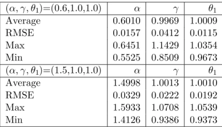
Table 3: Simulation Results for Regression
We set β = δ = 0.0 and setθ = (θ1, α, γ) in our simulations. The values of average, maximum, minimum, and RMSE of the MEL estimates are calculated from the estimates for each coefficients.
(α, γ, θ1)=(0.6,1.0,1.0) α γ θ1 Average 0.6010 0.9969 1.0009 RMSE 0.0157 0.0412 0.0115 Max 0.6451 1.1429 1.0354 Min 0.5525 0.8509 0.9673 (α, γ, θ1)=(1.5,1.0,1.0) α γ θ1 Average 1.4998 1.0013 1.0010 RMSE 0.0329 0.0222 0.0192 Max 1.5933 1.0708 1.0539 Min 1.4126 0.9386 0.9373 5. Conclusions
This paper first develops a new parameter estimation method of stable distribu-tions based on the empirical likelihood approach. We have shown that we can apply the empirical likelihood approach to the estimation problem of stable distributions and the computational burden is not heavy in comparison with the parametric maximum likelihood estimation. The maximum empirical likelihood (MEL) estimator for the pa-rameters of stable distributions has some desirable asymptotic properties; it has the consistency, the asymptotic normality, and the asymptotic efficiency when the num-ber of restrictions is large. Also it is possible to develop the empirical likelihood ratio statistics for the parameters of stable distributions which have the desirable asymp-totic property such as the asympasymp-totic χ2−distribution. Also we can construct a test procedure for the null-hypothesis of restrictions imposed and it is the same as the test
of overidentifying conditions in the econometrics literature.
Second, it is rather straightforward to extend our estimation method for unknown parameters of the stable distributions to the estimation of the general L´evy processes and the infinitely divisible distributions. It is also possible to apply it to the esti-mating equations problem with stable and infinitely divisible disturbance terms. We have shown that it is possible to estimate both the parameters of equations and the parameters of the distributions for disturbances at the same time by our method. It seems that it is not easy to solve this estimation problem by the conventional methods proposed in the past studies and in this sense our estimation method developed has some advantages over other methods.
Finally, we should mention that our estimation method is so simple that the re-sults can be extended to several directions. One obvious direction is to extend our method to the multivariate infinitely divisible distributions and it is straightforward to do it for the class of symmetric stable distributions. Although we have assumed that
Xk(k= 1,· · ·, n) are a sequence of i.i.d. random variables in this paper, there are many
interesting applications when they are dependent. Because there have been growing in-terests on the applications of the back-ground driving L´evy processes (BDLP) financial applications (Bandorff-Nielsen et. al. (2001)), these problems are under our current investigations
6. Mathematical Appendix
In this appendix we give the proofs of Theorem 2.2and Theorem 2.3 in Section 2. In our proof we have utilized some ideas of Kitamura et. al. (2001) and Hjort et. al. (2004) although their problem and formulation are quite different from ours. We first show the consistency of the MEL estimator, and then prove its asymptotic normality and asymptotic efficiency when m is large. Then akey lemma needed for the proof of Theorem 2.2 will be given and we utilize the proof of Theorem 2.2 to show Theorem 2.3. In our proofs we take a compact set Θ for the parameter space and we assume that the vector of true parameters θ0 is in Int(Θ) and each elements of Am(θ) and Bm(θ) are bounded.
Proof of Theorem 2.2:
[i] Consistency: We take a sufficiently large K (> 0) and set m = m(n) = [n13−],
0< <1/3, tl=K(l/m) (l= 1, . . ., m) in (2.4). Define a criterion function by
(6.1) Gn(θ) =−1 n n k=1 log[1 +Kλ(θ)g(Xk,θ)],
where the 2mrestrictions are given byg(Xk,θ) = (cos(t1Xk)−φRθ(t1), . . . ,cos(tmXk)−
φR
θ(tm),sin(t1Xk)−φIθ(t1), . . . ,sin(tmXk)−φIθ(tm) ) and the Lagrange multipliers
sat-isfy the equation as (2.9). Also define a function
u(θ) = KEθ0[g(X1,θ)] 1 +K Eθ0[g(X1,θ)] .
n∈N,we have (6.2) Eθ0[Ku(θ)g(X1,θ)] =K2 m l=1 φR θ0(tl)−φRθ(tl) 2 + φI θ0(tl)−φIθ(tl) 2 1 +K Eθ0[g(X1,θ)] >0.
For anyθ=θ0,we take a sufficiently smallδ >0,then forn∈N we have
Eθ0[supθ∗∈N B(θ0,δ)−Ku(θ∗)g(X1,θ∗)]<0,whereNB(θ0, δ) is an open ball with center
θ0 and radiusδ. Also supθ∈Θ|n−13+2Ku(θ)g(X1,θ)| ≤n−13+22K√2m and it goes to 0 asn→+∞. By using Taylor’s Theorem, there exists at∈(0,1) such that
−log1 +n−13+2Ku(θ)g(X1,θ =−n−13+2Ku(θ)g(X1,θ)+ n −2 3+(Ku(θ)g(X1,θ))2 2[1 +n−13+2tKu(θ)g(X1,θ)]2 and then (6.3) n13−2Eθ0 sup θ∗∈N B(θ0,δ) −log 1 +n−13+2Ku(θ∗)g(X1,θ∗) ≤ Eθ0 sup θ∗∈N B(θ0,δ) −Ku(θ∗)g(X1,θ∗) +Eθ0 sup θ∗∈N B(θ0,δ) n−13+2(Ku(θ∗)g(X1,θ∗))2 2[1 +tn−13+2Ku(θ∗)g(X1,θ∗)]2 .
Since n−13+2[Ku(θ)g(X1,θ)]2 ≤ 8K2n−31+2m and it goes to 0 as n → ∞, the sec-ond term of (6.3) converges to 0. By using (6.2), we can show that for any θ = θ0 and sufficiently small δ > 0, there exists n(θ, δ) such that for n ≥ n(θ, δ) we have
n13−2Eθ0{supθ∗∈N B(θ0,δ)−log[1 +n−
1
3+2Ku(θ∗)g(X1,θ∗)]} < 0. Since the set Θ\ NB(θ0, δ) is compact, there existL∈Band θ1,θ2, . . . ,θL such thatΘ\NB(θ0, δ)⊂
L
α=1NB(θα, δ). Then for anyn≥n(θα, δ) we have
(6.4) P 1 n n k=1 sup θ∗∈N B(θα,δ)− log[1 +n−13+2Ku(θ∗)g(Xk,θ∗)] > 1 3n −1 3+2Eθ0[ sup θ∗∈N B(θα,δ) −Ku(θ∗)g(X1,θ∗)] ≤ P 1 n n k=1 sup θ∗∈N B(θα,δ) −log[1 +n−13+2Ku(θ∗)g(Xk,θ∗)] −Eθ0{supθ∗∈N B(θα,δ)−log[1 +n− 1 3+2Ku(θ∗)g(X1,θ∗)]} >−1 6n −1 3+2Eθ 0[ sup θ∗∈N B(θα,δ)− Ku(θ∗)g(X1,θ∗)] ≤ 62 n13+
Varθ0{supθ∗∈N B(θα,δ)−log[1 +n−
1
3+2Ku(θ∗)g(X1,θ∗)]} (Eθ0[supθ∗∈N B(θα,δ)−Ku
(θ∗)g(X1,θ∗)])2 . We notice that the denominator of the right-hand side (RHS) of (6.4) does not converges to zero because of (6.2). Then by using the fact that RHS of (6.4) goes to 0, there
exists ¯n(θα, δ)∈Nsuch that for anyn≥n¯(θα, δ) it is less thanδ/2K (α= 1, . . . , L).
Hence for anyn≥max1≤β≤Ln¯(θβ, δ) we have P sup θ∗∈Θ\N B(θ0,δ) 1 n n k=1 −log[1 +n−13+2Ku(θ∗)g(Xk,θ∗)] > 1 3n −1 3+2 max 1≤β≤LEθ0[θ∗∈N Bsup(θβ,δ) −Ku (θ∗)g(X1,θ∗)] < δ2 . We notice thatλ(ˆθn) is the minimum of (2.6) and then we have the relation (6.5) P ⎛ ⎝ sup θ∗∈Θ\N B(θ0,δ) Gn(θ∗)> 1 3n −1 3+2 max 1≤β≤LEθ0[θ∗∈N Bsup(θβ,δ) −Ku(θ∗)g(X1,θ∗)] ⎞ ⎠< δ 2 .
Now we investigate the stochastic order of the Lagrange multipliers and we write them at the true value as λ(θ0) = λ(θ0) ξ, where ξ is the 2m×1 unit vector. By using the fact that the Lagrange multipliers are the solution of
(6.6) 1 n n k=1 Kg(Xk,θ0) 1 +Kλ(θ0)g(Xk,θ0) =0, we have (6.7) 0 = 1 m !! !! ! 1 n n k=1 Kg(Xk,θ0) 1 +Kλ(θ0)g(Xk,θ0) !! !! ! ≥ 1 m 1 nξ K n k=1 g(Xk,θ0)− λ(θ0) n k=1 K2g(Xk,θ0)ξg(Xk,θ0) 1 +K λ(θ0) ξg(Xk,θ0) ≥ λ(θ0) 1 +K λ(θ0) max1≤k≤n g(Xk,θ0) 1 n n k=1 K2 m ξ g(Xk,θ0)g(Xk,θ0) ξ −1 n n k=1 K mξ g(Xk,θ0) . We use the inequality Eθ0[(1/n)
n k=1ξ g(Xk,θ0) 2 ]≤(1/n)Eθ0[ g(X1,θ0) 2],which
is less thanm/n. Then we have the relation that (1/n)nk=1ξg(Xk,θ0)=Op(
" m/n). We define a 2m×2m matrix D(n) = (Dij(n)) by (6.8) D(n) = 1 n n k=1 K2 m g(Xk,θ0)g(Xk,θ0) −Eθ0[g(Xk,θ0)g(Xk,θ0) ] .
Then by using the Markov inequality we have the conditions that for any > 0
P(|Dij(n)| ≥) ≤c1(1/√n)2(1/m)2 and hence P(max1≤i,j≤n|Dij(n)| ≥) ≤c2(1/n),
whereci (i= 1,2) are some positive constants4 . Thus they converge to zero in
prob-ability as n−→ +∞. Also by using the similar arguments as (6.34) and Lemma A.1 below (we can take a sequence of nonsingular matrices as ˜W), we can show that the characteristic roots of 2m×2m matrixΣm(θ0) = (K2/m)Eθ0[g(Xk,θ0)g(Xk,θ0)
] are
positive and bounded both from the above and zero. Because
λ(θ0) /[1+K λ(θ0) max1≤k≤n g(Xk,θ0) ] =Op(
"
m/n) and max1≤k≤n g(Xk, θ0) ≤
2√2m=O(√m),we find thekey condition (6.9) λ(θ0) =Op( # m n) and (6.10) Gn(θ0)≥ − 1 n n k=1 Kλ(θ0)g(Xk,θ0) =−K λ(θ0) 1 n n k=1 ξg(Xk,θ0),
which is of the orderOp("m/n)Op("m/n) =op(n−13). Then there existsn ∈Nsuch that for anyn≥n we have
(6.11) P n13−2Gn(θ0)< n−2 max 1≤β≤LEθ0[θ∗∈N Bsup(θβ,δ)−Ku (θ∗)g(X1,θ∗)] < δ 2 .
Furthermore, by noting the fact that n13−2Gn(ˆθn) = supθ∗∈Θn13−2Gn(θ∗) (which is greater thann13−2Gn(θ0)) and using (6.11), we can evaluate
(6.12) P n13−2Gn(ˆθn)< n−2 max 1≤β≤LEθ0[θ∗∈N Bsup(θβ,δ) −Ku(θ∗)g(X1,θ∗)] < δ 2 .
Hence by combining (6.5) and (6.12), we have the conditionPθˆn∈/ NB(θ0, δ)
< δ ,
which implies that ˆθn−→p θ0 as n→+∞.
(ii)Asymptotic Normality : We consider the first order condition of the criterion function ∂Gn(ˆθn)/∂θ=0.Then by expanding −∂Gn(θ0)/∂θ around at ˆθn=θ0, we
have (6.13) −√n∂Gn(θ0) ∂θ = ∂2Gn(θ†n) ∂θ∂θ √ n(ˆθn−θ0),
where we have taken θ†n−θˆn ≤ ˆθn−θ0 . In order to show the asymptotic normality of the random vector−√n∂Gn(θ0)/∂θ,we write
(6.14) −√n∂Gn∂θ(θ0) = √n1 n n k=1 K 1 +Kλ(θ0)g(Xk,θ0) ∂g(Xk,θ0) ∂θ λ(θ0) = √n1 n n k=1 K 1 +Kλ(θ0)g(Xk,θ0) −∂Φθ0 ∂θ λ(θ0). By rewriting (6.6) with respect to the Lagrange multipliers, we have
(6.15) 0= 1 n n k=1 K mg(Xk,θ0)− 1 n n k=1 K2 m g(Xk,θ0)g(Xk,θ0) λ(θ0) +r1n,
where we set the remainder term
r1n= 1 n n k=1 K m g(Xk,θ0)(Kλ(θ0)g(Xk,θ0))2 1 +Kλ(θ0)g(Xk,θ0) .