Smooth Primal-Dual Coordinate Descent Algorithms
for Nonsmooth Convex Optimization
Ahmet Alacaoglu1 Quoc Tran-Dinh2 Olivier Fercoq3 Volkan Cevher1 1Laboratory for Information and Inference Systems (LIONS), EPFL, Lausanne, Switzerland
{ahmet.alacaoglu, volkan.cevher}@epfl.ch
2Department of Statistics and Operations Research, UNC-Chapel Hill, NC, USA [email protected]
3LTCI, Télécom ParisTech, Université Paris-Saclay, Paris, France [email protected]
Abstract
We propose a new randomized coordinate descent method for a convex optimization template with broad applications. Our analysis relies on a novel combination of four ideas applied to the primal-dual gap function: smoothing, acceleration, homotopy, and coordinate descent with non-uniform sampling. As a result, our method features the first convergence rate guarantees among the coordinate descent methods, that are the best-known under a variety of common structure assumptions on the template. We provide numerical evidence to support the theoretical results with a comparison to state-of-the-art algorithms.
1
Introduction
We develop randomized coordinate descent methods to solve the following composite convex problem: F?= min
x∈Rp
{F(x) =f(x) +g(x) +h(Ax)}, (1)
where f : Rp → R,g : Rp → R∪ {+∞}, andh : Rm → R∪ {+∞} are proper, closed and
convex functions,A∈Rm×pis a given matrix. The optimization template (1) covers many important
applications including support vector machines, sparse model selection, logistic regression, etc. It is also convenient to formulate generic constrained convex problems by choosing an appropriateh. Within convex optimization, coordinate descent methods have recently become increasingly popular in the literature [1–6]. These methods are particularly well-suited to solve huge-scale problems arising from machine learning applications where matrix-vector operations are prohibitive [1]. To our knowledge, there is no coordinate descent method for the general three-composite form (1) within our structure assumptions studied here that has rigorous convergence guarantees. Our paper specifically fills this gap. For such a theoretical development, coordinate descent algorithms require specific assumptions on the convex optimization problems [1, 4, 6]. As a result, to rigorously handle the three-composite case, we assume that (i)f is smooth, (ii)gis non-smooth but decomposable (each component has an “efficiently computable” proximal operator), and (iii)his non-smooth. Our approach: In a nutshell, we generalize [4, 7] to the three composite case (1). For this purpose, we combine several classical and contemporary ideas: We exploit the smoothing technique in [8], the efficient implementation technique in [4, 14], the homotopy strategy in [9], and the nonuniform coordinate selection rule in [7] in our algorithm, to achieve the best known complexity estimate for the template.
Surprisingly, the combination of these ideas is achieved in a very natural and elementary primal-dual gap-based framework. However, the extension is indeed not trivial since it requires to deal with the composition of a non-smooth functionhand a linear operatorA.
While our work has connections to the methods developed in [7, 10, 11], it is rather distinct. First, we consider a more general problem (1) than the one in [4, 7, 10]. Second, our method relies on Nesterov’s accelerated scheme rather than a primal-dual method as in [11]. Moreover, we obtain the first rigorous convergence rate guarantees as opposed to [11]. In addition, we allow using any sampling distribution for choosing the coordinates.
Our contributions:We propose a new smooth primal-dual randomized coordinate descent method for solving (1) wheref is smooth,gis nonsmooth, separable and has a block-wise proximal operator, andhis a general nonsmooth function. Under such a structure, we show that our algorithm achieves the best knownO(n/k)convergence rate, wherekis the iteration count and to our knowledge, this is the first time that this convergence rate is proven for a coordinate descent algorithm.
We instantiate our algorithm to solve special cases of (1) including the caseg= 0and constrained problems. We analyze the convergence rate guarantees of these variants individually and discuss the choices of sampling distributions.
Exploiting the strategy in [4, 14], our algorithm can be implemented in parallel by breaking up the full vector updates. We also provide a restart strategy to enhance practical performance.
Paper organization: We review some preliminary results in Section 2. The main contribution of this paper is in Section 3 with the main algorithm and its convergence guarantee. We also present special cases of the proposed algorithm. Section 4 provides numerical evidence to illustrate the performance of our algorithms in comparison to existing methods. The proofs are deferred to the supplementary document.
2
Preliminaries
Notation: Let[n] := {1,2,· · ·, n}be the set ofnpositive integer indices. Let us decompose the variable vectorxinton-blocks denoted byxiasx= [x1;x2;· · · ;xn]such that each blockxi
has the sizepi ≥ 1withPni=1pi = p. We also decompose the identity matrixIpofRpinton
block asIp = [U1, U2,· · · , Un], whereUi ∈ Rp×pi hasp
iunit vectors. In this case, any vector
x∈ Rpcan be written asx= Pni=1Uixi, and each block becomesxi = Ui>xfori ∈ [n]. We
define the partial gradients as∇if(x) =Ui>∇f(x)fori∈ [n]. For a convex functionf, we use
dom (f)to denote its domain,f∗(x) := supu
u>x−f(u) to denote its Fenchel conjugate, and
proxf(x) := arg minu
f(u) + (1/2)ku−xk2 to denote its proximal operator. For a convex set
X,δX(·)denotes its indicator function. We also need the following weighted norms:
kxik2(i)=hHixi, xii, (kyik∗(i)) 2=hH−1 i yi, yii, kxk2 [α] = Pn i=1L α ikxik2(i), (kyk ∗ [α]) 2 =Pn i=1L −α i (kyik∗(i)) 2. (2)
Here,Hi∈Rpi×piis a symmetric positive definite matrix, andL
i∈(0,∞)fori∈[n]andα >0.
In addition, we usek · kto denotek · k2.
Formal assumptions on the template: We require the following assumptions to tackle (1): Assumption 1. The functionsf,gandhare all proper, closed and convex. Moreover, they satisfy
(a) The partial derivative∇if(·)of f is Lipschitz continuous with the Lipschitz constant
ˆ
Li∈[0,+∞), i.e.,k∇if(x+Uidi)− ∇if(x)k(∗i)≤Lˆikdik(i)for allx∈Rp, di∈Rpi.
(b) The functiongis separable, which has the following formg(x) =Pn
i=1gi(xi).
(c) One of the following assumptions forhholds for Subsections 3.3 and 3.4, respectively: i. his Lipschitz continuous which is equivalent to the boundedness ofdom (h∗). ii. his the indicator function for an equality constraint, i.e.,h(Ax) :=δ{c}(Ax). Now, we briefly describe the main techniques used in this paper.
Acceleration: Acceleration techniques in convex optimization date back to the seminal work of Nesterov in [13], and is one of standard techniques in convex optimization. We exploit such a scheme to achieve the best knownO(1/k)rate for the nonsmooth template (1).
Nonuniform distribution: We assume thatξis a random index on[n]associated with a probability distributionq= (q1,· · · , qn)>such that
P{ξ=i}=qi>0, i∈[n], and n
X
i=1
Whenqi= 1nfor alli∈[n], we obtain the uniform distribution. Leti0, i1,· · · , ikbe i.i.d. realizations
of the random indexξafterkiteration. We defineFk+1=σ(i0, i1,· · · , ik)as theσ-field generated
by these realizations.
Smoothing techniques: We can write the convex functionh(u) = supy{hu, yi −h∗(y)}using
its Fenchel conjugateh∗. Sincehin (1) is convex but possibly nonsmooth, we smoothhas hβ(u) := max
y∈Rm
n
hu, yi −h∗(y)−β2ky−y˙k2o, (4)
wherey˙ ∈Rmis given andβ >0is the smoothness parameter. Moreover, the quadratic function
b(y,y˙) = 1 2ky−y˙k
2is defined based on a given norm in
Rm. Let us denote byyβ∗(u), the unique
solution of this concave maximization problem in (4), i.e.: y∗β(u) := arg max y∈Rm n hu, yi −h∗(y)−β 2ky−y˙k 2o= prox β−1h∗ y˙+β−1u , (5)
where proxh∗ is the proximal operator of h∗. If we assume thath is Lipschitz continuous, or equivalently thatdom (h∗)is bounded, then it holds that
hβ(u)≤h(u)≤hβ(u) + βD2
h∗
2 , where Dh∗ := max
y∈dom(h∗)ky−y˙k<+∞. (6) Let us define a new smoothed functionψβ(x) :=f(x) +hβ(Ax). Then,ψβis differentiable, and its
block partial gradient
∇iψβ(x) =∇if(x) +A>i y∗β(Ax) (7)
is also Lipschitz continuous with the Lipschitz constantLi(β) := ˆLi+k Aik2
β , whereLˆiis given in
Assumption 1, andAi∈Rm×piis thei-th block ofA.
Homotopy: In smoothing-based methods, the choice of the smoothness parameter is critical. This choice may require the knowledge of the desired accuracy, number of maximum iterations or the diameters of the primal and/or dual domains as in [8]. In order to make this choice flexible and our method applicable to the constrained problems, we employ a homotopy strategy developed in [9] for deterministic algorithms, to gradually update the smoothness parameter while making sure that it converges to0.
3
Smooth primal-dual randomized coordinate descent
In this section, we develop a smoothing primal-dual method to solve (1). Or approach is to combine the four key techniques mentioned above: smoothing, acceleration, homotopy, and randomized coordinate descent. Similar to [7] we allow to use arbitrary nonuniform distribution, which may allow to design a good distribution that captures the underlying structure of specific problems.
3.1 The algorithm
Algorithm 1 below smooths, accelerates, and randomizes the coordinate descent method. Algorithm 1.SMooth, Accelerate, Randomize The Coordinate Descent (SMART-CD) Input: Chooseβ1>0andα∈[0,1]as two input parameters. Choosex0∈Rp.
1 SetBi0:= ˆLi+kAik 2 β1 fori∈[n]. ComputeSα:= Pn i=1(B 0 i)αandqi:= (B 0 i) α Sα for alli∈[n].
2 Setτ0:= min{qi|1≤i≤n} ∈(0,1]fori∈[n]. Setx¯0= ˜x0:=x0.
3 fork←0,1,· · ·, kmaxdo
4 Updatexˆk := (1−τk)¯xk+τkx˜kand computeuˆk:=Axˆk.
5 Compute the dual stepy∗k :=y∗β
k+1(ˆu k) = prox β−k+11h∗ y˙+β −1 k+1uˆ k .
6 Select a block coordinateik ∈[n]according to the probability distributionq. 7 Setx˜k+1:= ˜xk, and compute the primalik-block coordinate:
˜ xki+1 k := argmin xik∈Rpik n h∇ikf(ˆx k) +A> iky ∗ k, xik−xˆ k iki+gik(xik) + τkBikk 2τ0 kxik−x˜ k ikk 2 (ik) o . 8 Updatex¯k+1:= ˆxk+τk τ0(˜x k+1−x˜k).
9 Computeτk+1 ∈(0,1)as the unique positive root ofτ3+τ2+τk2τ−τ
2 k = 0. 10 Updateβk+2:= 1+βkτ+1 k+1 andB k+1 i := ˆLi+kAik 2 βk+2 fori∈[n]. 11 end for
From the update¯xk := ˆxk−1+τk−1 τ0 (˜x k−x˜k−1)andxˆk := (1−τk)¯xk+τ kx˜k, it directly follows thatxˆk := (1−τ k) ˆxk−1+ τk−1 τ0 (˜x k−x˜k−1)
+τkx˜k. Therefore, it is possible to implement the
algorithm without formingx¯k.
3.2 Efficient implementation
While the basic variant in Algorithm 1 requires full vector updates at each iteration, we exploit the idea in [4, 14] and show that we can partially update these vectors in a more efficient manner. Algorithm 2.Efficient SMART-CD
Input: Choose a parameterβ1>0andα∈[0,1]as two input parameters. Choosex0∈Rp.
1 SetBi0:= ˆLi+kAik 2 β1 fori∈[n]. ComputeSα:= Pn i=1(B 0 i)αandqi:= (B0 i) α Sα for alli∈[n].
2 Setτ0:= min{qi|1≤i≤n} ∈(0,1]fori∈[n]andc0= (1−τ0). Setu0= ˜z0:=x0.
3 fork←0,1,· · ·, kmaxdo 4 Compute the dual stepy∗β
k+1(ckAu k+Az˜k) := prox β−1 k+1h∗ y˙+β −1 k+1(ckAuk+Az˜k) .
5 Select a block coordinateik ∈[n]according to the probability distributionq.
6 Let∇ki :=∇ikf(ckuk+ ˜zk) +A>iky ∗ βk+1(ckAu k+Az˜k). Compute tki+1 k := arg min t∈Rpik n h∇k i, ti+gik(t+ ˜z k ik) + τkBkik 2τ0 ktk 2 (ik) o . 7 Updatez˜ki+1 k := ˜z k ik+t k+1 ik . 8 Updateuki+1 k :=u k ik− 1−τk/τ0 ck t k+1 ik .
9 Computeτk+1 ∈(0,1)as the unique positive root ofτ3+τ2+τk2τ−τk2= 0. 10 Updateβk+2:= βk+1 1+τk+1 andB k+1 i := ˆLi+k Aik2 βk+2 fori∈[n]. 11 end for
We present the following result which shows the equivalence between Algorithm 1 and Algorithm 2, the proof of which can be found in the supplementary document.
Proposition 3.1. Letck=Q k
l=0(1−τl),zˆk=ckuk+ ˜zkandz¯k=ck−1uk+ ˜zk. Then,x˜k= ˜zk,
ˆ
xk= ˆzk andx¯k = ¯zk, for allk≥0, wherex˜k,xˆk, andx¯kare defined in Algorithm 1.
According to Algorithm 2, we never need to form or update full-dimensional vectors. Only times that we needxˆkare when computing the gradient and the dual variabley∗
βk+1. We present two special
cases which are common in machine learning, in which we can compute these steps efficiently. Remark 3.2. Under the following assumptions, we can characterize the per-iteration complexity explicitly. LetA, M ∈Rm×p, and
(a) fhas the formf(x) =Pm
j=1φj(e >
jM x), whereejis thejthstandard unit vector.
(b) h is separable as inh(Ax) =δ{c}(Ax)orh(Ax) =kAxk1.
Assuming that we store and maintain the residuals rk
u,f = M uk, rz,fk˜ = Mz˜k, rku,h = Auk,
rk
˜
z,h = Az˜
k, then we have the per-iteration cost asO(max{|{j | A
ji 6= 0}|,|{j | Mji 6= 0}|})
arithmetic operations. Ifhis partially separable as in [3], then the complexity of each iteration will remain moderate.
3.3 Case 1: Convergence analysis of SMART-CD for Lipschitz continuoush
We provide the following main theorem, which characterizes the convergence rate of Algorithm 1. Theorem 3.3. Let x? be an optimal solution of (1) and letβ
1 > 0 be given. In addition, let τ0 := min{qi|i∈[n]} ∈ (0,1]andβ0 := (1 +τ0)β1 be given parameters. For allk ≥1, the
sequencex¯k generated by Algorithm 1 satisfies:
EF(¯xk)−F?≤ C∗(x0) τ0(k−1) + 1 +β1(1 +τ0)D 2 h∗ 2(τ0k+ 1) , (8) whereC∗(x0) := (1−τ0)(Fβ0(x 0)−F?) +Pn i=1 τ0B0i 2qi kx ? i −x 0 ik 2 (i)andDh∗is as defined by(6).
In the special case when we use uniform distribution,τ0=qi= 1/n, the convergence rate reduces to EF(¯xk)−F?≤ nC∗(x0) k+n−1 + (n+ 1)β0Dh2∗ 2k+ 2n , whereC∗(x0) := (1− 1 n)(Fβ0(x 0)−F?) +Pn i=1 B0 i 2 kx ? i −x 0 ik 2
(i). This estimate shows that the convergence rate of Algorithm 1 is
On
k
, which is the best known so far to the best of our knowledge.
3.4 Case 2: Convergence analysis of SMART-CD for non-smooth constrained optimization In this section, we instantiate Algorithm 1 to solve constrained convex optimization problem with possibly non-smooth terms in the objective. Clearly, if we chooseh(·) =δ{c}(·)in (1) as the indicator function of the set{c}for a given vectorc∈Rm, then we obtain a constrained problem:
F?:= min x∈Rp
{F(x) =f(x) +g(x)|Ax=c}, (9)
wherefandgare defined as in (1),A∈Rm×p, andc∈ Rm.
We can specify Algorithm 1 to solve this constrained problem by modifying the following two steps: (a) The update ofy∗β
k+1(Axˆ k)at Step 5 is changed to yβ∗ k+1(Axˆ k) := ˙y+ 1 βk+1(Axˆ k−c), (10) which requires one matrix-vector multiplication inAxˆk.
(b) The update ofτkat Step 9 andβk+1at Step 10 are changed to
τk+1:=1+τkτk and βk+2:= (1−τk+1)βk+1. (11) Now, we analyze the convergence of this algorithm by providing the following theorem.
Theorem 3.4. Let
¯
xk be the sequence generated by Algorithm 1 for solving(9)using the updates
(10)and(11)and lety?be an arbitrary optimal solution of the dual problem of (9). In addition,
letτ0:= min{qi|i∈[n]} ∈(0,1]andβ0:= (1 +τ0)β1be given parameters. Then, we have the
following estimates: EF(¯xk)−F? ≤ C ∗(x0) τ0(k−1)+1+ β1ky?−y˙k2 2(τ0(k−1)+1) +ky ?k EkAx¯k−bk, EkAx¯k−bk ≤ τ0(kβ−11)+1 h ky?−y˙k+ ky?−y˙k2+ 2β−1 1 C∗(x0) 1/2i , (12) whereC∗(x0) := (1−τ 0)(Fβ0(x 0)−F?) +Pn i=1 τ0Bi0 2qi kx ?
i −x0ik2(i). We note that the following
lower bound always holds−ky?k
EkAx¯k−bk≤EF(¯xk)−F?.
3.5 Other special cases
We consider the following special cases of Algorithm 1:
The caseh= 0: In this case, we obtain an algorithm similar to the one studied in [7] except that we have non-uniform sampling instead of importance sampling. If the distribution is uniform, then we obtain the method in [4].
The caseg = 0: In this case, we haveF(x) = f(x) +h(Ax), which can handle the linearly constrained problems with smooth objective function. In this case, we can chooseτ0= 1, and the coordinate proximal gradient step, Step 7 in Algorithm 1, is simplified as
˜ xki+1 k := ˜x k ik− qik τkBkikH −1 ik ∇ikf(ˆx k) +A> iky ∗ βk+1(ˆu k). (13) In addition, we replace Step 8 with
¯
xki+1= ˆxki +τk
qi
(˜xki+1−x˜ki), ∀i∈[n]. (14) We then obtain the following results:
Corollary 3.5. Assume that Assumption 1 holds. Letτ0= 1,β1>0and Step 7 and 8 of Algorithm 1
be updated by(13)and(14), respectively. If, in addition,his Lipschitz continuous, then we have
EF(¯xk)−F?≤ 1 k n X i=1 B0 i 2q2 i kx?i −x0ik2 (i)+ β1D2h∗ k+ 1 , (15) whereDh∗is defined by(6).
If, instead of Lipschitz continuoush, we haveh(·) =δ{c}(·)to solve the constrained problem(9)
withg= 0, then we have
EF(¯xk)−F? ≤ C ∗(x0) k + β1ky?−y˙k2 2k +ky ?k EkAx¯k−bk, EkAx¯k−bk ≤ βk1 h ky?−y˙k+ ky?−y˙k2+ 2β−1 1 C∗(x 0)1/2i , (16) whereC∗(x0) := Pn i=1 B0 i 2q2 i kx? i −x0ik2(i). 3.6 Restarting SMART-CD
It is known that restarting an accelerated method significantly enhances its practical performance when the underlying problem admits a (restricted) strong convexity condition. As a result, we describe below how to restart (i.e., the momentum term) in Efficient SMART-CD. If the restart is injected in thek-th iteration, then we restart the algorithm with the following steps:
uk+1 ←0, ru,fk+1 ←0, ru,hk+1 ←0, ˙ y ←yβ∗ k+1(ckr k u,h+r k ˜ z,h), βk+1 ←β1, τk+1 ←τ0, ck ←1.
The first three steps of the restart procedure is for restarting the primal variable which is classical [15]. Restartingy˙is also suggested in [9]. The cost of this procedure is essentially equal to the cost of one iteration as described in Remark 3.2, therefore even restarting once every epoch will not cause a significant difference in terms of per-iteration cost.
4
Numerical evidence
We illustrate the performance of Efficient SMART-CD in brain imaging and support vector machines applications. We also include one representative example of a degenerate linear program to illustrate why the convergence rate guarantees of our algorithm matter. We compare SMART-CD with Vu-Condat-CD [11], which is a coordinate descent variant of Vu-Condat’s algorithm [16], FISTA [17], ASGARD [9], Chambolle-Pock’s primal-dual algorithm [18], L-BFGS [19] and SDCA [5].
4.1 A degenerate linear program: Why do convergence rate guarantees matter? We consider the following degenerate linear program studied in [9]:
min x∈Rp 2xp s.t. Pp−1 k=1xk = 1, xp−P p−1 k=1xk = 0, (2≤j≤d), xp≥0. (17)
Here, the constraint xp −Ppk−=11xk = 0 is repeatedd times. This problem satisfies the linear
constraint qualification condition, which guarantees the primal-dual optimality. If we define f(x) = 2xp, g(x) =δ{xp≥0}(xp), h(Ax) =δ{c}(Ax), where Ax= "p−1 X k=1 xk, xp− p−1 X k=1 xk, . . . , xp− p−1 X k=1 xk #> , c= [1,0, . . . ,0]>,
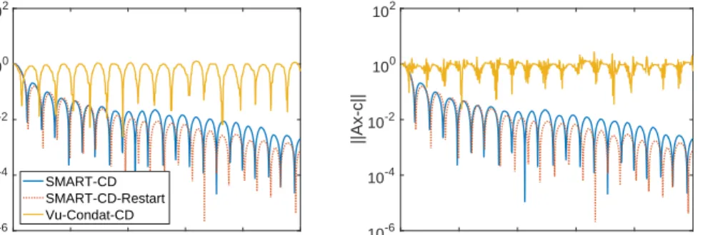
0 200 400 600 800 1000 epoch 10-6 10-4 10-2 100 102 F(x)-F * SMART-CD SMART-CD-Restart Vu-Condat-CD 0 200 400 600 800 1000 epoch 10-6 10-4 10-2 100 102 ||Ax-c||
Figure 1: The convergence behavior of3algorithms on a degenerate linear program. For this experiment, we select the dimensionsp= 10andd= 200. We implement our algorithm and compare it with Vu-Condat-CD. We also combine our method with the restarting strategy proposed above. We use the same mapping to fit the problem into the template of Vu-Condat-CD.
Figure 1 illustrates the convergence behavior of Vu-Condat-CD and SMART-CD. We compare primal suboptimality and feasibility in the plots. The explicit solution of the problem is used to generate the plot with primal suboptimality. We observe that degeneracy of the problem prevents Vu-Condat-CD from making any progress towards the solution, where SMART-CD preservesO(1/k)
rate as predicted by theory. We emphasize that the authors in [11] proved almost sure convergence for Vu-Condat-CD but they did not provide a convergence rate guarantee for this method. Since the problem is certainly non-strongly convex, restarting does not significantly improve performance of SMART-CD.
4.2 Total Variation and`1-regularized least squares regression with functional MRI data In this experiment, we consider a computational neuroscience application where prediction is done based on a sequence of functional MRI images. Since the images are high dimensional and the number of samples that can be taken is limited, TV-`1 regularization is used to get stable and predictive estimation results [20]. The convex optimization problem we solve is of the form:
min x∈Rp 1 2kM x−bk 2+λrkxk 1+λ(1−r)kxkTV. (18)
This problem fits to our template with f(x) =1
2kM x−bk
2, g(x) =λrkxk
1, h(u) =λ(1−r)kuk1,
whereDis the 3D finite difference operator to define a total variation normk · kTVandu=Dx. We use an fMRI dataset where the primal variablexis 3D image of the brain that contains33177
voxels. Feature matrixM has768rows, each representing the brain activity for the corresponding example [20]. We compare our algorithm with Vu-Condat’s algorithm, FISTA, ASGARD, Chambolle-Pock’s primal-dual algorithm, L-BFGS and Vu-Condat-CD.
0 20 40 60 80 100 time (s) 8000 8500 9000 9500 F(x) Chambolle-Pock Vu-Condat FISTA ASGARD L-BFGS Vu-Condat-CD SMART-CD 0 20 40 60 80 100 time (s) 8000 8500 9000 9500 F(x) 0 20 40 60 80 100 time (s) 8000 8500 9000 9500 F(x)
Figure 2: The convergence of7algorithms for problem (18). The regularization parameters for the first plot areλ= 0.001, r= 0.5, for the second plot areλ= 0.001, r= 0.9, for the third plot are λ= 0.01, r= 0.5.
Figure 2 illustrates the convergence behaviour of the algorithms for different values of the regu-larization parameters. Per-iteration cost of SMART-CD and Vu-Condat-CD is similar, therefore the behavior of these two algorithms are quite similar in this experiment. Since Vu-Condat’s,
Chambolle-Pock’s, FISTA and ASGARD methods work with full dimensional variables, they have slow convergence in time. L-BFGS has a close performance to coordinate descent methods. The simulation in Figure 2 is performed using benchmarking tool of [20]. The algorithms are tuned for the best parameters in practice.
4.3 Linear support vector machines problem with bias
In this section, we consider an application of our algorithm to support vector machines (SVM) problem for binary classification. Given a training set withmexamples{a1, a2, . . . , am}such that ai∈Rpand class labels{b1, b2, . . . bm}such thatbi ∈ {−1,+1}, we define the soft margin primal
support vector machines problem with bias as
min w∈Rp m X i=1 Cimax 0,1−bi(hai, wi+w0) +λ2kwk2. (19)
As it is a common practice, we solve its dual formulation, which is a constrained problem:
min x∈Rm 1 2λkM D(b)xk 2−Pm i=1xi s.t. 0≤xi≤Ci, i= 1,· · ·, m, b>x= 0, (20)
whereD(b)represents a diagonal matrix that has the class labelsbiin its diagonal andM ∈Rp×mis
formed by the example vectors. If we define f(x) = 1 2λkM D(b)xk 2− m X i=1 xi, gi(xi) =δ{0≤xi≤Ci}, c= 0, A=b >,
then, we can fit this problem into our template in (9).
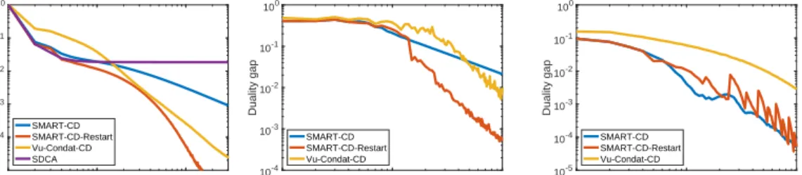
We apply the specific version of SMART-CD for constrained setting from Section 3.4 and compare with Vu-Condat-CD and SDCA. Even though SDCA is a state-of-the-art method for SVMs, we are not able to handle the bias term using SDCA. Hence, it only applies to (20) whenb>x= 0constraint is removed. This causes SDCA not to converge to the optimal solution when there is bias term in the problem (19). The following table summarizes the properties of the classification datasets we used.
Data Set Training Size Number of Features Convergence Plot rcv1.binary [21, 22] 20,242 47,236 Figure 3, plot 1 a8a [21, 23] 22,696 123 Figure 3, plot 2 gisette [21, 24] 6,000 5,000 Figure 3, plot 3
Figure 3 illustrates the performance of the algorithms for solving the dual formulation of SVM in (20). We compute the duality gap for each algorithm and present the results with epochs in the horizontal axis since per-iteration complexity of the algorithms is similar. As expected, SDCA gets stuck at a low accuracy since it ignores one of the constraints in the problem. We demonstrate this fact in the first experiment and then limit the comparison to SMART-CD and Vu-Condat-CD. Equipped with restart strategy, SMART-CD shows the fastest convergence behavior due to the restricted strong convexity of (20). 100 101 102 epoch 10-4 10-3 10-2 10-1 100 Duality gap SMART-CD SMART-CD-Restart Vu-Condat-CD SDCA 100 101 102 epoch 10-4 10-3 10-2 10-1 100 Duality gap SMART-CD SMART-CD-Restart Vu-Condat-CD 100 101 102 epoch 10-5 10-4 10-3 10-2 10-1 100 Duality gap SMART-CD SMART-CD-Restart Vu-Condat-CD
Figure 3: The convergence of4algorithms on the dual SVM (20) with bias. We only used SDCA in the first dataset since it stagnates at a very low accuracy.
5
Conclusions
Coordinate descent methods have been increasingly deployed to tackle huge scale machine learning problems in recent years. The most notable works include [1–6]. Our method relates to several works
in the literature including [1, 4, 7, 9, 10, 12]. The algorithms developed in [2–4] only considered a special case of (1) withh= 0, and cannot be trivially extended to apply to general setting (1). Here, our algorithm can be viewed as an adaptive variant of the method developed in [4] extended to the sum of three functions. The idea of homotopy strategies relate to [9] for first-order primal-dual methods. This paper further extends such an idea to randomized coordinate descent methods for solving (1). We note that a naive application of the method developed in [4] to the smoothed problem with a carefully chosen fixed smoothness parameter would result in the complexityO(n2/k), whereas using our homotopy strategy on the smoothness parameter, we reduced this complexity toO(n/k). With additional strong convexity assumption on problem template (1), it is possible to obtainO(1/k2)
rate by using deterministic first-order primal-dual algorithms [9, 18]. It remains as future work to incorporate strong convexity to coordinate descent methods for solving nonsmooth optimization problems with a faster convergence rate.
Acknowledgments
The work of O. Fercoq was supported by a public grant as part of the Investissement d’avenir project, reference ANR-11-LABX-0056-LMH, LabEx LMH. The work of Q. Tran-Dinh was partly supported by NSF grant, DMS-1619884, USA. The work of A. Alacaoglu and V. Cevher was supported by European Research Council (ERC) under the European Union’s Horizon 2020 research and innovation programme (grant agreement no725594 - time-data).
References
[1] Y. Nesterov, “Efficiency of coordinate descent methods on huge-scale optimization problems,”
SIAM Journal on Optimization, vol. 22, no. 2, pp. 341–362, 2012.
[2] P. Richtárik and M. Takáˇc, “Iteration complexity of randomized block-coordinate descent methods for minimizing a composite function,”Mathematical Programming, vol. 144, no. 1-2, pp. 1–38, 2014.
[3] P. Richtárik and M. Takáˇc, “Parallel coordinate descent methods for big data optimization,”
Mathematical Programming, vol. 156, no. 1-2, pp. 433–484, 2016.
[4] O. Fercoq and P. Richtárik, “Accelerated, parallel, and proximal coordinate descent,”SIAM Journal on Optimization, vol. 25, no. 4, pp. 1997–2023, 2015.
[5] S. Shalev-Shwartz and T. Zhang, “Stochastic dual coordinate ascent methods for regularized loss minimization,”Journal of Machine Learning Research, vol. 14, pp. 567–599, 2013. [6] I. Necoara and D. Clipici, “Parallel random coordinate descent method for composite
mini-mization: Convergence analysis and error bounds,”SIAM J. on Optimization, vol. 26, no. 1, pp. 197–226, 2016.
[7] Z. Qu and P. Richtárik, “Coordinate descent with arbitrary sampling i: Algorithms and com-plexity,”Optimization Methods and Software, vol. 31, no. 5, pp. 829–857, 2016.
[8] Y. Nesterov, “Smooth minimization of non-smooth functions,”Math. Prog., vol. 103, no. 1, pp. 127–152, 2005.
[9] Q. Tran-Dinh, O. Fercoq, and V. Cevher, “A smooth primal-dual optimization framework for nonsmooth composite convex minimization,”arXiv preprint arXiv:1507.06243, 2015. [10] O. Fercoq and P. Richtárik, “Smooth minimization of nonsmooth functions with parallel
coordinate descent methods,”arXiv preprint arXiv:1309.5885, 2013.
[11] O. Fercoq and P. Bianchi, “A coordinate descent primal-dual algorithm with large step size and possibly non separable functions,”arXiv preprint arXiv:1508.04625, 2015.
[12] Y. Nesterov and S.U. Stich, “Efficiency of the accelerated coordinate descent method on structured optimization problems,”SIAM J. on Optimization, vol. 27, no. 1, pp. 110–123, 2017. [13] Y. Nesterov, “A method for unconstrained convex minimization problem with the rate of
convergenceO(1/k2),”Doklady AN SSSR, vol. 269, translated as Soviet Math. Dokl., pp. 543– 547, 1983.
[14] Y. T. Lee and A. Sidford, “Efficient accelerated coordinate descent methods and faster algorithms for solving linear systems,” inFoundations of Computer Science (FOCS), 2013 IEEE Annual Symp. on, pp. 147–156, IEEE, 2013.
[15] B. O’Donoghue and E. Candes, “Adaptive restart for accelerated gradient schemes,”Foundations of computational mathematics, vol. 15, no. 3, pp. 715–732, 2015.
[16] B. C. V˜u, “A splitting algorithm for dual monotone inclusions involving cocoercive operators,”
Advances in Computational Mathematics, vol. 38, no. 3, pp. 667–681, 2013.
[17] A. Beck and M. Teboulle, “A fast iterative shrinkage-thresholding algorithm for linear inverse problems,”SIAM journal on imaging sciences, vol. 2, no. 1, pp. 183–202, 2009.
[18] A. Chambolle and T. Pock, “A first-order primal-dual algorithm for convex problems with applications to imaging,”Journal of mathematical imaging and vision, vol. 40, no. 1, pp. 120– 145, 2011.
[19] R. H. Byrd, P. Lu, J. Nocedal, and C. Zhu, “A limited memory algorithm for bound constrained optimization,”SIAM Journal on Scientific Computing, vol. 16, no. 5, pp. 1190–1208, 1995. [20] E. D. Dohmatob, A. Gramfort, B. Thirion, and G. Varoquaux, “Benchmarking solvers for tv-`1
least-squares and logistic regression in brain imaging,” inPattern Recognition in Neuroimaging, 2014 International Workshop on, pp. 1–4, IEEE, 2014.
[21] C.-C. Chang and C.-J. Lin, “Libsvm: a library for support vector machines,”ACM transactions on intelligent systems and technology (TIST), vol. 2, no. 3, p. 27, 2011.
[22] D. D. Lewis, Y. Yang, T. G. Rose, and F. Li, “Rcv1: A new benchmark collection for text categorization research,”Journal of Machine Learning Research, vol. 5, no. Apr, pp. 361–397, 2004.
[23] M. Lichman, “UCI machine learning repository,” 2013.
[24] I. Guyon, S. Gunn, A. Ben-Hur, and G. Dror, “Result analysis of the nips 2003 feature selection challenge,” inAdvances in neural information processing systems, pp. 545–552, 2005. [25] P. Tseng, “On accelerated proximal gradient methods for convex-concave optimization,”
Supplementary document
Smooth Primal-Dual Coordinate Descent Algorithms for
Nonsmooth Convex Optimization
A
Key lemmas
The following properties are key to design the algorithm, whose proofs are very similar to the proof of [9, Lemma 10] by using a different norm, and we omit the proof here. The proof of the last property directly follows by using the explicit form ofhβ(u)in the special case whenh∗(y) =hc, yi. Lemma A.1. For anyu,uˆ∈Rm, the functionhβdefined by(4)satisfies the following properties:
(a) hβ(·)is convex and smooth. Its gradient∇hβ(u) =yβ∗(u)is Lipschitz continuous with the Lipschitz constantLhβ = 1 β. (b) hβ(u) +h∇hβ(u),uˆ−ui+β2ky∗β(u)−y∗β(ˆu)k2≤hβ(ˆu). (c) h(ˆu)≥hβ(u) +h∇hβ(u),uˆ−ui+β2ky∗β(u)−y˙k 2. (d) hβ(u)≤hβ¯(u) + β¯−β 2 kyβ∗(u)−y˙k2.
(e) Ifh∗(y) =hc, yi, a linear function, thenhβ(u) =hβ¯(u) + ( ¯β−β)β
2 ¯β ky
∗
β(u)−y˙k
2.
Lemma A.2. The parameters{τk}k≥0and{βk}k≥1updated by Steps 9 and 10, respectively, satisfy
the following bounds:
1 k+τ0−1 ≤τk≤ 2 k+τ0−1+ 1, βk ≤ β1(1 +τ0) τ0k+ 1 . (21)
Proof. We proceed by induction. By Step 9, we haveτ2
k−1=
τ3
k+τ
2
k
1−τk . Fork= 0, the bounds trivially
hold sinceτ0 ≤ n1. By the inductive assumption, we have k−1+1τ−1 0
≤τk−1 ≤ k+2τ−1 0
. Assume toward condtradiction thatτk <k+1τ−1
0 . Then(k 1 −1+τ−1 0 )2 ≤τ2 k−1= τk3+τk2 1−τk < k+1+τ−1 0 (k+τ−1 0 )2(k−1+τ −1 0 ) , which is a contradiction. Thereforeτk≥ k+1τ−1
0
. For the other side of the inequality, assume toward contradiction thatτk >k+1+2τ−1 0 . Then 4(k+3+τ −1 0 ) (k+1+τ0−1)2(k−1+τ−1 0 ) < τk3+τ 2 k 1−τk =τ 2 k−1≤ 4 (k+τ0−1)2, which is a contradiction. Therefore,τk ≤k+1+2τ−1 0 . For{βk}, we note thatβk= 1+βkτ−1
k−1 =β1 Qk−1 i=1 1 1+τi ≤β1 Qk−1 i=1 i+τ−1 0 i+1+τ0−1 = β1(1+τ0) τ0k+1 .
The following lemma is motivated by [4]. Lemma A.3. Consider the iterates{¯xk,x˜k}k
≥0of Algorithm 1. Then, fork≥0andi∈[n], we
can write{¯xk i}as a convex combination of{˜xli}kl=0: ¯ xki = k X l=0 γik,lx˜li, (22) whereγik,l≥0andPk l=0γ k,l
i = 1. Moreover, the coefficientsγ k,l
i can explicitly be computed as
γik+1,l= (1−τk)γ k,l i , forl= 0,· · ·, k−1, (1−τk)γik,k+τk−ττk 0, forl=k, τk τ0, forl=k+ 1. (23)
Proof. Now, from the definition ofx¯k+1andxˆk, fori∈[n], we can write ¯ xki+1= (1−τk)¯xki +τkx˜ki + τk τ0 (˜xki+1−x˜ki) = (1−τk)¯xki + (τk− τk τ0 )˜xki + τk τ0 ˜ xki+1. (24)
We prove thatx¯ki =Pk
l=0γ
k,l i x˜
l
ifori∈ [n]such thatγ k,l i ≥0and Pk l=0γ k,l i = 1. Indeed, for
k = 0, we have x¯0 = ˜x0, which trivially holds if we chooseγ0,0
i = 1. Now, assume that this
expression holds fork ≥1, we prove it holds fork+ 1. Indeed, from (24), using this induction assumption, we can write
¯ xki+1= (1−τk) k−1 X l=0 γik,lx˜li+ (1−τk)γ k,k i +τk− τk τ0 ˜ xki +τk τ0 ˜ xki+1= k+1 X l=0 γki+1,lx˜li, where constants γki+1,l are as given in (23). It is trivial to check that Pk+1
l=0 γ k+1,l i = (1− τk)P k l=0γ k,l
i +τk−ττk0 +ττk0 = (1−τk) +τk = 1. In addition, since{τk}k≥0is a non-increasing sequence,γik,l≥0.
B
Convergence analysis of SMART-CD
B.1 The proof of Theorem 3.3First, let us define the full primal proximal-gradient step as
¯ ˜ xk+1:= arg min x∈Rp ( h∇ψβk+1(ˆx k), x−xˆki+g(x) +τ k n X i=1 Bk i 2τ0 kxi−x˜kik2(i) ) , (25) where∇ψβk+1(ˆx k) =∇f(ˆxk) +A>y∗ βk+1(Axˆ
k). The primal coordinate step (Step 7) and Step 8 in
Algorithm 1 can be written as
˜ xki+1= ¯ ˜ xki+1, if i=ik, ˜ xk i, otherwise. (26) Moreover, using [25, Property 2], we know that for allx∈Rpand for alli∈[n],
gi(¯x˜ki+1)≤gi(xi) +h∇iψβk+1(ˆx k ), xi−x¯˜ki+1i+ τkBik 2τ0 kxi−x˜kik 2 (i)− kxi−x¯˜ki+1k 2 (i) −τkB k i 2τ0 kx¯˜ki+1−x˜kik2 (i). (27)
Now, since the partial gradient∇ikfisLˆik-Lipschitz continuous, usingx¯
k+1 ik = ˆx k ik+ τk τ0(˜x k+1 ik −x˜ k ik)
andx¯ki+1= ˆxki fori6=ik, we have
f(¯xk+1)≤f(ˆxk) +h∇ikf(ˆx k),x¯k+1 ik −xˆ k iki+ ˆ Lik 2 k¯x k+1 ik −xˆ k ikk 2 (ik) =f(ˆxk) +τk τ0 h∇ikf(ˆxk),x˜ki+1 k −x˜ k iki+ τk2Lˆik 2τ2 0 kx˜ki+1 k −x˜ k ikk 2 (ik). (28)
Taking theFk-conditional expectation with respect toikand noting (26), we obtain Eik f(¯xk+1)| Fk ≤f(ˆxk) +τk τ0 n X i=1 qih∇if(ˆxk),x˜¯ki+1−x˜kii +τ 2 k τ2 0 n X i=1 qi ˆ Li 2 k ¯ ˜ xki+1−x˜kik 2 (i). (29)
Next, let us denote byϕβ(x) :=hβ(Ax). Then, by Lemma A.1, we can see thatϕβk+1has
block-coordinate Lipschitz gradient with the Lipschitz constant kAik2
βk+1, whereAiis thei-th column block
ofA. Moreover,∇iϕβk+1(x) =A > i yβ∗k+1(Ax). Hence, usingx¯ k+1 ik = ˆx k ik+ τk τ0(˜x k+1 ik −x˜ k ik)and ¯
xki+1= ˆxki fori6=ik, we can write
ϕβk+1(¯x k+1) ≤ϕβk+1(ˆx k) + h∇ikϕβk+1(ˆx k),x¯k+1 ik −xˆ k iki+ kAik2 2βk+1 k¯xki+1 k −xˆ k ikk 2 (ik) =ϕβk+1(ˆx k) +τk τ0 h∇ikϕβk+1(ˆx k),x˜k+1 ik −x˜ k iki+ τ2 kkAik2 2τ2 0βk+1 kx˜ki+1 k −x˜ k ikk 2 (ik).
Taking theFk-conditional expectation with respect toikgivenFkand noting (26), we get Eik ϕβk+1(¯x k+1)| Fk ≤ϕβk+1(ˆx k) +τk τ0 n X i=1 qih∇iϕβk+1(ˆx k),x¯˜k+1 i −x˜ k ii +τ 2 k τ2 0 n X i=1 qi kAik2 2βk+1 kx¯˜ki+1−x˜kik2 (i). (30) Now, we define ˆ gik:= k X l=0 γik,lgi(˜xli) and ˆgk := n X i=1 ˆ gik. (31)
Using Lemma A.3, we can write
ˆ gik+1= k+1 X l=0 γik+1,lgi(˜xli) = k−1 X l=0 (1−τk)γik,lgi(˜x l i) + h (1−τk)γik,k+τk−ττk 0 i gi(˜xki) +τk τ0 gi(˜xki+1) = (1−τk) k X l=0 γik,lgi(˜xli) +τkgi(˜xki) + τk τ0 gi(˜xki+1)−gi(˜xki) = (1−τk)ˆgki +τkgi(˜xki) + τk τ0 gi(˜xki+1)−gi(˜xki).
Using the definition (31) ofgˆk, this estimate implies ˆ gk+1= (1−τk)ˆgk+ n X i=1 τkgi(˜xki) + τk τ0 gi(˜xki+1)−gi(˜xki) . Now, by the expression (26), we can show that
Eik
gi(˜xki+1)| Fk
=qigi(¯x˜ki+1) + (1−qi)gi(˜xki).
Combining the two last expressions, we can derive
Eik ˆ gk+1| Fk = (1−τk)ˆgk+ n X i=1 τkgi(˜xki) + τk τ0 E ik gi(˜xki+1)| Fk −gi(˜xki) = (1−τk)ˆgk+τk n X i=1 gi(˜xki) +τk τ0 n X i=1 qi gi(¯x˜ki+1)−gi(˜x k i) . (32) Let us defineFˆk βk:=f(¯x k) + ˆgk+h βk(Ax¯ k)≡f(¯xk) + ˆgk+ϕ βk(¯x
k). Then, from (29), (30) and
(32), we have that Eik h ˆ Fβk+1 k+1| Fk i =Eik f(¯xk+1)| Fk +Eik ˆ gk+1| Fk +Eik ϕβk+1(¯x k+1) | Fk ≤ " f(ˆxk) +τk τ0 n X i=1 qih∇if(ˆxk),x¯˜ki+1−x˜ k ii # + " ϕβk+1(ˆx k) +τk τ0 n X i=1 qih∇iϕβk+1(ˆx k),x¯˜k+1 i −x˜ k ii # + " (1−τk)ˆgk+τk n X i=1 gi(˜xki) +τk τ0 n X i=1 qi gi(¯x˜ki+1)−gi(˜x k i) # + τ 2 k 2τ2 0 n X i=1 qi ˆ Li+ kAik2 βk+1 kx¯˜ki+1−x˜kik 2 (i), (33)
since∇ψβk+1(ˆx
k) =∇f(ˆxk) +∇ϕ βk+1(ˆx
k). Now, using the estimate (27) into the last expression
and noting thatBki = ˆLi+kAik 2
βk+1 , we can further derive that for allx,
Eik h ˆ Fβk+1 k+1| Fk i ≤ " f(ˆxk) +τk τ0 n X i=1 qih∇if(ˆxk), xi−x˜kii # + " ϕβk+1(ˆx k) +τk τ0 n X i=1 qih∇iϕβk+1(ˆx k), x i−x˜kii # + " (1−τk)ˆgk+τk n X i=1 gi(˜xki) + τk τ0 n X i=1 qi gi(xi)−gi(˜xki) # + n X i=1 qi τ2 kB k i 2τ2 0 kxi−x˜kik 2 (i)− kxi−x¯˜ki+1k 2 (i) . (34)
Let us choosexsuch that for alli∈[n],xi=
1−τ0 qi ˜ xk i + τ0 qix ?
i. Note that asτ0≤qifor alli,xi
is a convex combination ofx˜ki andx?i. We obtain
Eik h ˆ Fβk+1 k+1|Fk i ≤ f(ˆxk) +τkh∇f(ˆxk), x?−x˜ki + ϕβk+1(ˆx k) +τkh∇ϕ βk+1(ˆx k), x?−x˜ki + (1−τk)ˆgk+τkg(x?) + n X i=1 qi τ2 kB k i 2τ2 0 τ0 qi (x?i −x˜ki) 2 (i) − 1−τ0 qi ˜ xki + τ0 qi x?i −x¯˜ k+1 i 2 (i) ! . (35)
We simplify the norm difference using the fact thatkax+ (1−a)y−zk2 =akx−zk2+ (1− a)ky−zk2−a(1−a)kx−yk2. 1−τ0 qi ˜ xki +τ0 qi x?i −x¯˜k+1 i 2 (i) = 1−τ0 qi k˜xki −x¯˜k+1 i k 2 (i)+ τ0 qi kx?i −x¯˜k+1 i k 2 (i)− 1−τ0 qi τ 0 qi k˜xki −x?ik2 (i) ≥ τ0 qi kx?i −x¯˜k+1 i k 2 (i)− 1−τ0 qi τ 0 qi k˜xki −x?ik2 (i). and we get Eik h ˆ Fβk+1 k+1 |Fk i ≤ f(ˆxk) +τkh∇f(ˆxk), x?−x˜ki +hϕβk+1(ˆx k) +τ kh∇ϕβk+1(ˆx k), x? −x˜kii +(1−τk)ˆgk+τkg(x?) + n X i=1 τk2Bik 2τ0 kx?i −x˜kik2 (i)− kx¯˜ k+1 i −x ? ik 2 (i) . (36)
Using the convexity off, we havef(ˆxk) +h∇f(ˆxk), x?−xˆki ≤f(x?)andf(ˆxk) +h∇f(ˆxk),x¯k− ˆ
xki ≤f(¯xk). Moreover, sincexˆk = (1−τk)¯xk+τkx˜k, we haveτk(x?−x˜k) = (1−τk)(¯xk− ˆ
xk) +τk(x?−xˆk). Combining these expressions, we obtain
f(ˆxk) +τkh∇f(ˆxk), x?−x˜ki ≤(1−τk)f(¯xk) +τkf(x?). (37)
On the one hand, by the Lipschitz gradient and convexity ofϕβk+1in Lemma A.1(b), we have
ϕβk+1(ˆx k) +h∇ϕ βk+1(ˆx k),x¯k−xˆki ≤ϕ βk+1(¯x k)−βk+1 2 ky ∗ βk+1(Axˆ k)−y∗ βk+1(Ax¯ k)k2.
On the other hand, by Lemma A.1(c), we also have ϕβk+1(ˆx k) + h∇ϕβk+1(ˆx k), x? −xˆki ≤h(Ax?)−βk+1 2 ky ∗ βk+1(Axˆ k) −y˙k2
Combining these two inequalities and usingτk(x?−x˜k) = (1−τk)(¯xk−xˆk) +τk(x?−xˆk), we get ϕβk+1(ˆx k) +τkh∇ϕ βk+1(ˆx k), x?−x˜ki ≤(1−τk)ϕ βk+1(¯x k) +τ kh(Ax?) −(1−τk)βk+1 2 ky ∗ βk+1(Axˆ k)−y∗ βk+1(Ax¯ k)k2−τkβk+1 2 ky ∗ βk+1(Axˆ k)−y˙k2. Next, using Lemma A.1(d), we can further estimate
ϕβk+1(ˆx k) +τ kh∇ϕβk+1(ˆx k), x?−x˜ki ≤(1−τk)ϕ βk(¯x k) +τ kh(Ax?) −(1−τk)βk+1 2 ky ∗ βk+1(Axˆ k) −y∗β k+1(Ax¯ k )k2−τkβk+1 2 ky ∗ βk+1(Axˆ k) −y˙k2 +(1−τk)(βk−βk+1) 2 ky ∗ βk+1(Ax¯ k)−y˙k2 ≤(1−τk)ϕβk(¯x k) +τ kh(Ax?) −1 2(βk+1τk(1−τk)−(1−τk)(βk−βk+1))ky ∗ βk+1(Ax¯ k)−y˙k2. (38) Here, in the last inequality, we use the fact that(1−τ)ka−bk2+τkak2−τ(1−τ)kbk2 =
ka−(1−τ)bk2≥0for anya,b, andτ∈[0,1]. Substituting (37) and (38) into (36), we obtain
Eik h ˆ Fβk+1 k+1 | Fk i ≤(1−τk)f(¯xk) + ˆgk+ϕβk(¯x k) +τk[f(x?) +g(x?) +h(Ax?)] + n X i=1 τ2 kBki 2τ0 kx?i −x˜kik2 (i)− kx ? i −x¯˜ k+1 i k 2 (i) −(1−τk) 2 [βk+1(1 +τk)−βk]ky ∗ βk+1(Ax¯ k)−y˙k2. (39)
Next, let us denote byQk:=P n i=1 τ2 kBki 2τ0 h kx?i −x˜kik2 (i)− kx ? i −x¯˜ k+1 i k 2 (i) i
. We can further express Qkas Qk = n X i=1 τ2 kBki 2τ0 h kx?i −x˜kik2 (i)− kx ? i −x¯˜ k+1 i k 2 (i) i =Eik " τ2 kBkik 2qikτ0 kx?i k−x˜ k ikk 2 (ik)− kx ? ik−x˜ k+1 ik k 2 (ik) | Fk # =Eik " n X i=1 τ2 kBik 2qiτ0 kx?i −x˜kik2 (i)− kx ? i −x˜ k+1 i k 2 (i) | Fk # , (40)
where the last equality follows from the fact thatx˜ki+1= ˜xk
i fori6=ik.
Substituting this expression into (39) and using the definition ofFˆk βkandF ?:=F(x?) =f(x?) + g(x?) +h(Ax?), we get Eik " ˆ Fβk+1 k+1+ n X i=1 τk2Bik 2qiτ0 kx?i −x˜ki+1k2 (i)| Fk # ≤(1−τk) ˆFβkk+τkF(x?) + n X i=1 τ2 kB k i 2qiτ0 kx?i −x˜kik2(i)− Rk, whereRk := (1−τk) 2 [βk+1(1 +τk)−βk]ky ∗ βk+1(Ax¯
k)−y˙k2. Assume that we chooseβ
kandτk
such thatβk+1(1 +τk)−βk ≥0, thenRk ≥0. Taking the expected value of the last estimate over
theσ-fieldFk, we obtain
E h ˆ Fβk+1 k+1−F ?i+ E " n X i=1 τ2 kBik 2qiτ0 kx?i−˜xki+1k2 (i) # ≤(1−τk)E h ˆ Fβk k−F ?i +E " n X i=1 τ2 kB k i 2qiτ0 kx?i −x˜ k ik 2 (i) # . (41)
In order to telescope this inequality we assume that τk2Bik ≤ (1−τk) τk2−1B k−1 i , which is equivalent to τk2 ˆ Li+ kAik2 βk+1 ≤(1−τk) τk2−1 ˆ Li+ kAik2 βk . (42) Let us updateβk+1= 1+βkτ
k. Then, this condition becomes
τk2βkLˆi+(1+τk)kAik2
≤(1−τk)τk2−1βkLˆi+kAik2
. (43)
The condition (43) holds ifτ2
k(1 +τk) = (1−τk)τk2−1. Hence, we can computeτkas the unique
positive root ofτ3+τ2+τ2
k−1τ −τ 2
k−1 = 0. By Lemma A.2, the root of this cubic satisfies 1 k+τ0−1 ≤τk ≤ 2 k+τ0−1+1. Let us defineSk = Pn i=1 τ2 kBik 2qiτ0kx ? i −x˜ k+1 i k 2
(i). Then, we can recursively show that E h ˆ Fβk+1 k+1−F ?+S k i ≤ k Y i=1 (1−τi)E " ˆ Fβ11−F?+ n X i=1 τ2 0B0i 2qiτ0 kx?i −x˜1ik2 (i) # ≤ k Y i=1 (1−τi) (1−τ0)( ˆFβ00−F ?) + n X i=1 τ02Bi0 2qiτ0 kx?i −x˜0ik2(i) ! ,
where the second inequality follows from (41). Sinceτk≥ k+1τ−1 0
, it is trivial to show thatωk+1:=
Qk i=1(1−τi)≤ Qk i=1 i+τ0−1−1 i+τ0−1 = 1 τ0k+1. Now, we haveFβ0(x 0) =f(x0) +g(x0) +h β0(Ax 0) = ˆ F0 β0, andx˜
0 = x0. In addition, by the convexity ofg and Lemma A.3, we also haveg(¯xk) =
gPk
l=0γk,lx˜l
≤Pk
l=0γk,lg(˜xl) = ˆgk. Hence, we can write the above estimate as
EFβk(¯x k)−F? ≤ 1 τ0(k−1) + 1 " (1−τ0)(Fβ0(x 0)−F?) + n X i=1 τ0Bi0 2qi kx?i −x0ik2 (i) # . (44)
Now, using the bound (6), we have0≤F(¯xk)−F?≤F βk(¯x
k)−F?+β k
D2h∗
2 . Combining this estimate and the above inequality, and noting thatβk ≤ β1τ(1+τ0)
0k+1 by Lemma A.2, we obtain the
bound in (8).
B.2 The proof of Theorem 3.4
Sinceh(u) =δ{c}(u), we can smooth this function ashβ(u) = maxy
n
hu−c, yi −β
2ky−y˙k 2o. Let us first defineSβ(x) :=E[F(x) +hβ(Ax)−F?]. Sinceh∗(y) =hc, yi, we use Lemma A.1(e)
to estimate (38) in the proof of Theorem 3.3 instead of Lemma A.1(d) to obtain ϕβk+1(ˆx k) +τkh∇ϕ βk+1(ˆx k), x?−x˜ki ≤(1−τk)ϕ βk(¯x k) +τ kh(Ax?) −(1−τk)βk+1 2βk [βk+1−(1−τk)βk]kyβ∗k+1(Ax¯ k)−y˙k2. (45) Hence, ifβk+1= (1−τk)βk, thenϕβk+1(ˆx k) +τ kh∇ϕβk+1(ˆx k), x?−˜xki ≤(1−τ k)ϕβk(¯x k) +
τkh(Ax?). Now, we combine the conditionβk+1= (1−τk)βkand (42), we can show that
τk2 (1−τk)βkLˆi+kAik2 ≤(1−τk)2τk2−1 βkLˆi+kAik2 . This condition holds ifτk2= (1−τk)2τk2−1, which leads toτk=
τk−1
τk−1+1. This is the update rule (11)
of the algorithm. It is trivial to show thatτk= k+1τ−1 0
andβk= τ β1
0(k−1)+1. Now, we apply (44) to
obtain the bound Sβk(¯x k)≤ C∗ τ0(k−1) + 1 , where C∗:= (1−τ0)(Fβ0(x 0)−F?) + n X i=1 τ0Bi0 2qi kx?i −x0ik2 (i).
Now, let us define the dual problem of (1) as max y∈Rm min x∈Rp F(x) +hAx, yi −h∗(y) , (46)
and denote an optimal point of (46) asy?. We defineD
βk(x) :=F(x) +hβk(Ax)−F
?and apply
[9, Lemma 1] to obtain algorithm-independent duality bounds
F(¯xk)−F? ≤D βk(¯x k) +ky?k Ax¯k−b +β2kky?−y˙k 2 , kAx¯k−bk ≤β k h ky?−y˙k+ ky?−y˙k2+ 2β−1 k Dβk(¯x k)1/2i . (47)
The result in (12) follows by taking the expectation and using the concavity of the square-root and
Jensen’s inequality.
B.3 The proof of Corollary 3.5
From the update in (13), we get the trivial inequality, similar to (27), that τkBki 2qi kx¯˜ki+1−x˜kik2(i)≤ h∇iψβk+1(ˆx k), x? i −x¯˜ k+1 i i +τkB k i 2qi kx¯˜k+1 i −x ? ik 2 (i)− k˜x k i −x ? ik 2 (i) . (48)
Due to the specific Step 8 in Section 3.5, instead of (33), we get
Eik h ˆ Fβk+1 k+1| Fk i =Eik f(¯xk+1)| Fk +Eik ˆ gk+1| Fk +Eik ϕβk+1(¯x k+1) | Fk ≤ " f(ˆxk) +τk n X i=1 h∇if(ˆxk),x¯˜ki+1−x˜ k ii # + " ϕβk+1(ˆx k) +τ k n X i=1 h∇iϕβk+1(ˆx k),x¯˜k+1 i −x˜ k ii # + n X i=1 τ2 k 2qi ˆ Li+ kAik2 βk+1 kx¯˜k+1 i −x˜ k ik 2 (i). (49)
Plugging(48) into the last inequality gives us
Eik h ˆ Fβk+1 k+1 | Fk i =Eik f(¯xk+1)| Fk +Eik ˆ gk+1| Fk +Eik ϕβk+1(¯x k+1)| F k ≤ f(ˆxk) +τkh∇f(ˆxk), x?−x˜ki + ϕβk+1(ˆx k) +τ kh∇ϕβk+1(ˆx k), x? −x˜ki + n X i=1 τ2 kB k i 2qi kx?i −x˜kik2 (i)− kx ? i −x¯˜ k+1 i k 2 (i) . (50) If we letQk :=Pni=1 τ2 kBki 2qi kx? i −x˜kik2(i)− kx ? i −x¯˜ k+1 i k2(i)
, then similar to (40), we get
Qk =Eik " n X i=1 τ2 kBik 2q2 i kx?i −x˜kik2 (i)− kx ? i −x˜ k+1 i k 2 (i) | Fk # . (51)
Consequently, by using the same updates forτkandβk, the recursion in (41) becomes
E h ˆ Fβk+1 k+1−F ?i+ E " n X i=1 τ2 kBik 2q2 i kx?i−˜xki+1k2 (i) # ≤(1−τk)E h ˆ Fβk k−F ?i +E " n X i=1 τ2 kB k i 2q2 i kx?i −x˜ k ik 2 (i) # . (52)
Hence, we finally get EFβk(¯x k)−F? ≤ 1 τ0(k−1) + 1 " (1−τ0)(Fβ0(x 0)−F?) + n X i=1 τ2 0B0i 2q2 i kx?i −x0ik2 (i) # . Noting thatτ0= 1, we get
Sβk(¯x k) ≤ C ∗ k , where C ∗:= n X i=1 B0 i 2q2 i kx?i −x0ik2(i). (53)
By using the bound of{βk}k≥1as in Lemma A.2, we obtain the bound (15). For the constrained case, we use (53) on (47), with the specific update rule of{βk}for the constrained case, to obtain (16)
using the same arguments as in the Proof of Theorem 3.4.
C
Equivalence of SMART-CD and Efficient SMART-CD
In this appendix, we give a proof by induction for the equivalence of Algorithm 1 and Algorithm 2 motivated by [4].
C.1 The proof of Proposition 3.1
The claim trivially holds fork= 0using the initialization of the parameters. Assume that the relations hold for somek. Using Step 7 of Algorithm 2, we have
˜ zki+1 k = ˜z k ik+t k+1 ik . (54)
We can write from Step 6 of Algorithm 2 that tki+1 k = arg min t∈Rpik h∇ikf(cku k+ ˜zk) +A> iky ∗ βk+1 ckAu k+Az˜k , ti+gik(t+ ˜z k ik) +τkB k ik 2τ0 ktk2 (ik) = arg min t∈Rpik h∇ikf(ˆzk) +A>iky∗βk+1 Azˆk, ti+gik(t+ ˜z k ik) + τkBikk 2τ0 ktk2 (ik) = arg min t∈Rpik h∇ikf(ˆxk) +A>iky∗βk+1 Axˆk , ti+gik(t+ ˜x k ik) + τkBkik 2τ0 ktk2 (ik) =−˜xkik+ arg min x∈Rpik h∇ikf(ˆxk) +A>iky∗βk+1 Axˆk, x−xˆkiki+gik(x) +τkB k ik 2τ0 kx−x˜kikk2 (ik) =−˜xkik+ ˜xki+1 k .
By (54) and the inductive assumption onx˜k, we obtain ˜
zk+1= ˜xk+1. Next, using the definition ofz¯k+1and Step 8, we can derive
¯ zk+1=ckuk+1+ ˜zk+1=ck uk− 1−τk/τ0 ck (˜zk+1−z˜k) + ˜zk+1 =ckuk+ ˜zk+ τk τ0 (˜zk+1−z˜k) = ˆzk+τk τ0 (˜zk+1−z˜k) = ˆxk+τk τ0 (˜xk+1−x˜k) = ¯xk+1.
Finally, we use the definition ofzˆk+1,ckand Step 9 of Algorithm 1, we arrive at ˆ zk+1=ck+1uk+1+ ˜zk+1 = ck+1 ck (¯xk+1−z˜k+1) + ˜zk+1 = (1−τk+1)(¯zk+1−z˜k+1) + ˜zk+1 = (1−τk+1)(¯xk+1−x˜k+1) + ˜xk+1 = (1−τk+1)¯xk+1+τk+1x˜k+1 = ˆxk+1.