Does Private Tutoring Payoff?

IZA DP No. 3637

Does Private Tutoring Payoff?

Ayfer Gurun

Daniel L. Millimet

DISCUSSION P

APER SERIES

Forschungsinstitut zur Zukunft der Arbeit Institute for the Study of Labor

Does Private Tutoring Payoff?

Ayfer Gurun

Southern Methodist University

Daniel L. Millimet

Southern Methodist University

and IZA

Discussion Paper No. 3637

August 2008

Any opinions expressed here are those of the author(s) and not those of IZA. Research published in this series may include views on policy, but the institute itself takes no institutional policy positions.

The Institute for the Study of Labor (IZA) in Bonn is a local and virtual international research center and a place of communication between science, politics and business. IZA is an independent nonprofit organization supported by Deutsche Post World Net. The center is associated with the University of Bonn and offers a stimulating research environment through its international network, workshops and conferences, data service, project support, research visits and doctoral program. IZA engages in (i) original and internationally competitive research in all fields of labor economics, (ii) development of policy concepts, and (iii) dissemination of research results and concepts to the interested public.

IZA Discussion Papers often represent preliminary work and are circulated to encourage discussion. Citation of such a paper should account for its provisional character. A revised version may be available directly from the author.

IZA Discussion Paper No. 3637

August 2008

ABSTRACT

Does Private Tutoring Payoff?

We assess the causal effect of private tutoring on the probability of university placement in

Turkey. We find that tutoring increases the probability of being placed in a university when

non-random selection is ignored. Moreover, among those utilizing private tutoring, greater

expenditure on tutoring is also positively associated with university placement. However, we

find evidence of positive selection into tutoring, but negative selection into greater

expenditures among those receiving tutoring. Accounting for this pattern of non-random

selection, we conclude that private tutoring has a negative causal effect on university

placement overall, but conditional on receiving any tutoring, spending more on tutoring has a

positive causal effect on university placement.

JEL Classification:

C31, H51, I21, O15

Keywords:

tutoring, Turkey, tertiary education, program evaluation

Corresponding author:

Daniel L. Millimet

Department of Economics

Southern Methodist University

Box 0496

Dallas, TX 75275-0496

USA

E-mail: millimet@mail.smu.edu

1

Introduction

The evolution of private tutoring – fee-based tutoring outside the normal school day that provides supple-mentary instruction to students in academic subjects –has proliferated around the world. It became popular initially in Asia several decades ago, and has since spread to Africa, Europe, and North America (Dang and Rogers 2008).1 This growth has encountered mixed reactions from policymakers and educational researchers. First and foremost, it is unclear if private tutoring has a bene…cial, causal e¤ect on academic achievement. Second, if it does, this raises concerns regarding educational equity and limitations on intergenerational income mobility. Finally, private tutoring, particularly when it is done by teachers outside of school, creates an incentive for teachers to provide lower quality education within the public school system. In this study, we exploit a unique database from Turkey to examine the …rst and second concerns.

Bray and Kwok (2003) and Bray (1999) review private tutoring schemes across a diverse set of countries. One stylized fact is that private tutoring is more common in countries with competitive university entrance examinations (Tansel and Bircan 2006). In many countries, the combination of these high stakes exams and shortcomings of the educational system (e.g., insu¢ cient supply of universities, large class sizes, and inadequate public resources) are also mentioned as salient factors underlying the demand for private tutoring (Tansel and Bircan 2006). Moreover, demand for private tutoring is not solely con…ned to developing countries (Bray and Kwok 2003). Here, the poor performance by students on international achievement tests is given as a contributing factor to the growth in demand.

In Turkey, the government is responsible for providing formal education at all levels, including the compulsory level (primary and secondary school) and high school.2 _{There does exist an active private} sector in formal education especially in urban areas. Public and private schools are governed by the Ministry of Education. Due to a limited supply of tertiary education, a national university entrance exam is required of all high school graduates to gain access to university education.

The demand for private tutoring in Turkey emanates from the competitive university placement exam-ination (Tansel and Bircan 2006). There exist three types of private tutoring in Turkey: (i) one-on-one instruction by a privately paid teacher, (ii) formal courses o¤ered by teachers after regular school hours, and (iii) private …rms o¤ering lessons by professional teachers in a classroom setting. Although the …rst and second types are frequently utilized, they are not regulated. The third type is the most common; fa-cilities of this exist across the country (Tansel and Bircan 2006). Students attend these fafa-cilities outside the regular school day, and they are noted for smaller classes, improved class materials, and more e¤ective student-teacher interactions compared to formal schools (Tansel and Bircan 2006).

The number of private tutoring centers has proliferated over the past two decades (Tansel and Bircan 2006). In 1984 there were less than 200 such centers across the country. After a 1984 legal reform recognizing 1_{Surveys covering the extent of private tutoring in selected countries can be found in Dang (2007a, b) and Dang and Rogers} (2008).

2_{See Tansel and Bircan (2006) for a detailed review of the educational setup in Turkey. Tansel and Bircan (2008) provide} a detailed account of the history of private tutoring centers.

these private tutoring centers as part of educational activities, the number of centers quickly grew, reaching more than 2,000 in 2002 (Private Tutoring Centers Association 2003). For comparison, there were roughly 2,500 high schools in Turkey at the time (Ministry of Education of Turkey 2003).

The average fee charged by private tutoring centers in preparation for the university entrance examination was approximately $1,300 US dollars in 2002 (Tansel and Bircan 2006). For comparison, per capita income in Turkey was 2,500 US dollars in 2002. Aggregate tutoring expenditures correspond to 1.44% of GDP, or $263 million US dollars, and is comparable to total public sector educational spending (Tansel and Bircan 2006).

To understand the determinants of private tutoring, and its impact on university placement, we use survey data administrated by the Turkish Higher Education Council in 2002 merged with data on actual test outcomes. More than ten percent of the 1.2 million students taking the 2002 university entrance exam were required to complete the survey. The survey contains information on demographic attributes, educational background, and private tutoring. These data allow us to investigate two interesting issues. First, how e¤ective is tutoring in gaining university placement? Second, who invests in tutoring?

Our analysis complements several existing studies using data from Turkey and elsewhere. Tansel and Bircan (2006) analyze expenditures on private tutoring in Turkey utilizing cross-sectional data from 1994. Kim and Lee (2004) similarly analyze expenditures in South Korea using two data sets from 1997 and 1998. Tansel and Bircan (2005) utilize the same data set as we do and assess the association between private tutoring and university placement and test scores in Turkey. The authors conclude that private tutoring is bene…cial, but the treatment of tutoring as exogenous is suspect. Kang (2007) assesses the e¤ect of private tutoring in South Korea on student academic achievement. The author attempts to circumvent the potential endogeneity of tutoring using an indicator for …rst born status as an instrument. While the instrument is fairly strong, birth order may directly a¤ect academic achievement. Nonetheless, the e¤ect of tutoring is imprecisely measured and not statistically signi…cant. Finally, Dang (2007b) uses data from Vietnam in the 1990s to analyze determinants of private tutoring demand and its impact on academic achievement. The author utilizes the cost of tutoring charged by schools as an exclusion restriction, …nding a positive e¤ect of tutoring on academic performance.

In light of these previous studies, it is seems prudent to assess the role of non-random selection into tutoring in Turkey prior to inferring a causal e¤ect of tutoring in that country. There are several reasons why we should be concerned about selection on unobservables in the Turkish case. As in South Korea and Vietnam, students receiving private tutoring may di¤er along various unobserved, but salient, dimensions from those who abstain from tutoring. For example, parents who purchase tutoring for their children may also aid their children’s academic success in other ways (e.g., helping with homework). In addition, more motivated students may be more willing to enroll in private tutoring than their less motivated peers, and this motivation may translate into better academic performance even absent tutoring. However, the selection process may also work in the opposite direction. For example, students attending lower quality high schools,

or who otherwise anticipate not performing well on the university placement exam, may be more willing to incur the cost of private tutoring.

Unfortunately, however, there does not seem to be any valid exclusion restriction in our data. To proceed, then, we employ several recently developed parametric and semi-nonparametric techniques from the program evaluation literature. These techniques allow us to assess the impact of non-random selection on the estimated treatment e¤ects obtained under exogeneity. Our results show that non-random selection is an important issue. First, we …nd evidence of positive selection into private tutoring in general, but negative selection into high expenditure on tutoring. Second, a modest amount of positive selection on unobservables into tutoring is su¢ cient to explain the positive association between tutoring and university placement; in fact, the treatment e¤ect actually becomes negative and statistically signi…cant. However, the positive association between high expenditure on tutoring and university placement is robust to the presence of selection on unobservables. Since it is only high expenditure on tutoring that pays o¤, our results have signi…cant rami…cations for thinking about the current education system in Turkey, educational equity and intergenerational mobility. The remainder of the paper is organized as follows. Section 2 discusses the empirical framework and data. Section 3 presents the results. Section 4 concludes.

2

Empirics

2.1

Data

We use a survey administrated by the Turkish Higher Education Council in 2002 to more than ten percent of the 1.2 million students taking the 2002 university entrance exam. Our sample includes 90,410 students taking the exam for the …rst time. We focus on …rst-time test takers since the factors in‡uencing the university placement of students taking the exam multiple times may be in‡uenced by other factors that are not applicable to …rst-time takers.

We use placement to a university after the exam as our measure of academic achievement. We de…ne two binary treatment variables. The …rst treatment variable, denoted Tutor I, takes on a value of one if the student receives any private tutoring prior to the exam (zero otherwise). The second treatment variable – denoted Tutor II and de…ned only for the subset of students receiving any private tutoring – takes on a value of one if the student spent more than $1,275 US dollars on private tutoring prior to the exam, and a value of zero if the student spent less than $1,275 (but more than zero).3 _{Thus, the …rst treatment allows} us to assess the overall impact of private tutoring, while the second treatment allows to assess the impact of greater expenditure on private tutoring conditional on receiving any tutoring.

To control for parental and environmental factors, we include a number of covariates in the analysis. Categorical variables are included for the number of siblings, mother’s and father’s education, family income, primary and secondary test scores, and city population. In addition, dummy variables are included for gender

and internet access.4 _{We exclude students with missing data for gender. Missing values for the remaining} control variables are imputed (replaced by zero) and imputation dummies are added to the control set.5

Summary statistics are provided in Table 1. In our sample of 90,410 students, 80.1% received private tutoring. Of these, 46,262 indicated a monetary amount, with 13.1% spending more than $1,275 US dollars. Given the relatively high percentage of observations with missing data on total expenditures on private tutoring, one should be concerned with the representativeness of the sample when analyzing the second treatment. Thus, Table 1 provides separate summary statistics for individuals withTutor II missing versus non-missing, as well as the p-values from t-tests of equal means. The results indicate that students with non-missing data clearly di¤er in a statistically and economically meaningful way from those with missing data. For example, students with missing data are much less likely to have internet access and high previous academic achievement; they are more likely to reside in less a- uent households as measured by income and parental education, have more siblings, and reside in less populous areas. While we can control for these regressors in the analysis, it is likely that students with missing data also di¤er along unobservable dimensions as well. As such, the results using theTutor II treatment should be interpreted cautiously. We shall return to this below.

2.2

Methodology

2.2.1 Parametric Estimation

We begin by specifying the following regression model

yi= I(xi + Di+"i>0) (1)

where y is a binary measure of observed university placement, xis a vector of controls, D represents one of the treatments being analyzed, and are parameters to be estimated, with being the parameter of primary interest, and " is the error term. Probit estimation of (1) yields a consistent estimate of if, conditional onx, Cov(D; ") = 0and"i

iid

N(0;1).

Even if the distributional assumption concerning "is correct, it is well known that D and"will not be independent conditional onxif individuals select into the treatment on the basis of unobservable attributes. The standard approach to so-called selection on unobservables is to utilize instrumental variables. However, in the current context, it is unlikely that there are any valid exclusion restrictions in the data. Instead, we borrow various strategies from the program evaluation literature to assess the sensitivity of our probit estimates to selection on unobservables. To assess the impact of non-random selection into tutoring, we 4_{Number of siblings takes values between one and …ve, where …ve represents “more than …ve siblings.” Mother’s and father’s} education each take values between one (no education) and seven (Master’s/Ph.d.), where higher values indicate more education. Family income takes values between one (lowest) and seven (highest). Primary and secondary school test scores each take values between one (highest) and four (lowest). Finally, city population takes values between one (smallest) to nine (largest).

5_{Number of siblings and family income are missing for less than 1% of the sample; primary and secondary test scores are} missing for less than 4% of the sample; mother’s and father’s education are missing for 6% and 8% of the sample, respectively; and, population is missing for 8% of the sample.

employ the bivariate probit model utilized in Altonji et al. (2005, 2008). The model is given by

yi = I(xi + Di+"i>0) (2)

Di = I(xi + i>0)

where is the error term in the treatment assignment equation.

Bivariate probit estimation of (2) yields a consistent estimate of if, conditional onx,"i; i iid

N2(0;0;1;1; ).

The correlation coe¢ cient, , captures the correlation between unobservables that impact university place-ment and the likelihood of receiving the treatplace-ment; >0 ( < 0) implies positive (negative) selection on unobservables. Aside from the estimate of , estimates of and provide information on who receives private tutoring.

Given the bivariate normality assumption, the model is technically identi…ed even absent an exclusion restriction; semi-parametric alternatives require an exclusion restriction. As such, to assess the role of selection into treatment without formally relying on the distributional assumption, Altonji et al. (2005, 2008) treat the model as underidenti…ed by one parameter, . Then, the authors constrain to di¤erent values and examine the estimates of the remaining parameters; constraining to be zero yields estimates under selection on observables only. We proceed along similar lines.

2.2.2 Semi-Nonparametric Estimation

The preceding estimator requires one to specify a functional form for the outcome equation, as well as distributions for the error terms. To relax these assumptions, we turn to two related, but distinct, semi-nonparametric estimation techniques. To understand both techniques, it is useful to explicitly consider the potential outcomes framework (see, e.g., Neyman 1923; Fisher 1935; Roy 1951; Rubin 1974). Lety1i denote the potential outcome (i.e., university placement) of studentiunder the treatment (D= 1);y0idenotes the potential outcome absent the treatment (D= 0). The student-speci…c causal e¤ect of the treatment is given by the di¤erence between the corresponding potential outcomes, i=y1i y0i; the average treatment e¤ect

(ATE) is given by AT E= E[ i].

For each student, the observed outcome, yi, is equivalent to yi = Diy1i + (1 Di)y0i. Thus, some

identifying assumptions are needed to circumvent the missing counterfactual problem. Under the conditional independence assumption (CIA), treatment assignment is assumed to be independent of potential outcomes conditional on the set of observed covariates, x. Rosenbaum and Rubin (1983) show that independence conditional onximplies independence conditional on the propensity score, p(xi) = Pr(Di = 1jxi).

Two popular classes of propensity score-based estimators of the ATE under the CIA are weighting estimators and matching estimators.6 _{Because selection into treatment on the basis of unobservables will} bias estimates of the ATE under either type of estimator, both of the estimation techniques below assess the

sensitivity of the estimates obtained under CIA to violations of this assumption. Thus, the logic is identical to the Altonji et al. (2005, 2008) approach discussed above in the context of parametric estimation.

Minimum Bias Inverse Propensity Score Weighting Our …rst estimation approach applies the tech-nique recently proposed in Millimet and Tchernis (2008), who build on Black and Smith (2004). Intuitively, the idea is to utilize a weighting estimator applied to a properly chosen sub-set of the original sample in order to minimize the bias arising from failure of the CIA.

To begin, Hirano and Imbens (2001) propose the following (normalized) weighting estimator of the ATE:

^HI = "_N X i=1 yiDi b p(xi) , _N X i=1 Di b p(xi) # "_N X i=1 yi(1 Di) 1 p_b(xi) , _N X i=1 (1 Di) 1 p_b(xi) # ; (3)

wherep_b(xi)is an estimate of the propensity score (obtain, for example, using a probit model). This estimator yields an unbiased estimate of AT E under CIA. To examine the bias when CIA fails, assume the following:

(A1) Potential outcomes and latent treatment assignment are additively separable in observables and unob-servables y0 = g0(x) +"0 y1 = g1(x) +"1 D = h(x) D = 8 < : 1 ifD >0 0 otherwise (A2) "0; "1; N3(0; ), where = 2 6 6 6 4 2 0 01 0 2 1 1 1 3 7 7 7 5:

Under (A1) and (A2), Millimet and Tchernis (2008) show that the bias of the ATE, conditional onp(x), due to failure of the CIA is given by

BAT E[p(x)] = 0 0 (h(x)) (h(x))[1 (h(X))] + [1 (h(x))] u (h(x)) (h(x))[1 (h(x))] = _{f 0} 0+ [1 (h(x))] g (h(x)) (h(x))[1 (h(x))] : (4)

where p(x) = (h(x)), = "1 "0 (i.e., individual-speci…c, unobserved gains from treatment), and u is the correlation between and .

with a propensity score in a neighborhood aroundp , the value of the propensity score that minimizes (4). Formally, the authors propose the followingminimum biased estimator of the ATE:

^M B[p ] = " X i2 yiDi b p(xi) , X i2 Di b p(xi) # " X i2 yi(1 Di) 1 _bp(xi) , X i2 (1 Di) 1 p_b(xi) # (5) where =_fi_jbp(xi)2C(p )g; andC(p)denotes a neighborhood aroundp. We de…neC(p )as

C(p ) =_fp_b(xi)jpb(xi)2(p; p)g;

where p = max_f0:02; p _g, p = min_f0:98; p + _g, and > 0 is the smallest value such that at least percent of both the treatment and control groups are contained in . In the analysis, we set

= 0:01;0:03;0:05, 0:10, and 0:25. For example, if = 0:01, we …nd the smallest value, 0:01, such that

1% of the treatment group and 1% of the control group have a propensity score in the interval(p; p). Thus, smaller values of should reduce the bias at the expense of higher variance.7

To implement this technique,p must be estimated. The procedure in Millimet and Tchernis (2008) calls for estimating p assuming (A1), (A2), and functional forms for g0(x),g1(x), andh(x)using the Heckman

bivariate normal (BVN) selection model. Speci…cally, assuming

g0(x) = x 0 g1(x) = x 1 h(X) = x then yi=xi 0+xiDi( 1 0) + 0(1 Di) (xi ) 1 (xi ) + ₁Di (xi ) (xi ) + _i (6)

where ( )= ( )is the inverse Mills’ratio, is a mean zero error term, and

0 = 0 0 (7)

1 = 0 0+ :

Thus, OLS estimation of (6) after replacing with an estimate obtained from a …rst-stage probit model yields consistent estimates of ₀ 0 and . With these estimates, one can use (4) to obtain an estimate

7_{We trim observations with propensity scores above (below) 0.98 (0.02), regardless of the value of , to prevent any single} observations from receiving too large of a weight.

of p . Millimet and Tchernis (2008) verify the virtues of this technique even if the functional form and distributional assumptions underlying the BVN selection model are mis-speci…ed, and even if CIA holds. A con…dence interval for the minimum biased estimate of the ATE is obtained using 200 bootstrap repetitions.

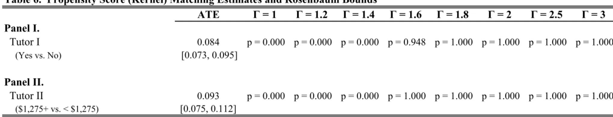
Propensity Score Matching For our …nal estimation technique, we estimate the ATE using propensity score matching along with Rosenbaum bounds (Rosenbaum 2002). While there exist other methods of assess-ing the sensitivity of PSM estimates to selection on unobservables, Rosenbaum bounds are computationally attractive and also o¤er an intuitively appealing measure of the way in which unobservables enter the model (Ferraro et al. 2007). To implement the matching estimator, we use kernel weighting with the normal kernel and a …xed bandwidth of 0.10. Con…dence intervals are obtained using 200 bootstrap repetitions.

To understand the Rosenbaum bounds, let i represent the odds of student i receiving the treatment (i.e., receiving private tutoring); i=(1 i)is the odds ratio. Assume the log odds ratio can be expressed as a generalized function of observables,xi, and a binary, unobserved term, i. Formally,

ln i

(1 i)

= (xi) + i (8)

Thus, the relative odds ratio of two observationally identical students is given by

i (1 i) j (1 j) = expf (xi) + ig exp_f (xj) + jg = exp_f ( i j)g (9)

which di¤ers from unity if and i j is non-zero . Moreover, since is binary, i j 2 f 1;0;1g, and

1 exp_{f g}

i(1 j) j(1 i)

exp_{f g} (10)

If exp_{f g}= 1, as it would in a randomized experiment or in non-experimental data free of bias from selection on unobservables, the model is said to be free of hidden bias; controlling for selection on observables would yield an unbiased estimate of the treatment e¤ect. Higher values of imply an increasingly important role of unobservables in the treatment selection process. For example, = 2 implies that observationally identical students di¤er in their relative odds of treatment by a factor of two. Rosenbaum bounds use bounds on the distribution of Wilcoxen’s signed rank statistic under the null of zero treatment e¤ect using di¤erent values of . This leads to bounds on the signi…cance level of a one-sided test for no treatment e¤ect.

3

Results

3.1

Bivariate Probit Estimates

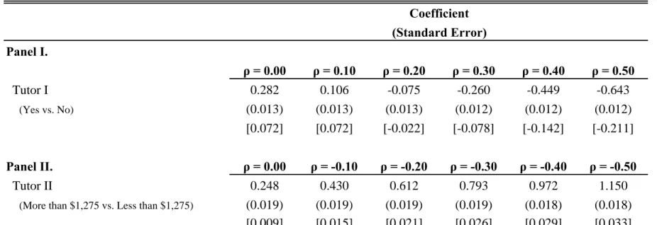
Table 2 presents the results obtained from the constrained bivariate probit model; Tables 3 and 4 present the unconstrained estimates. Panel I in Table 2 and Table 3 contain the results using the …rst treatment:

any tutoring versus no tutoring prior to the exam (denotedTutor I). Panel II in Table 2 and Table 4 contain the results using the second treatment: tutoring expenditures of at least $1,275 US dollars versus tutoring expenditures less than $1,275 US dollars but greater than zero prior to the exam (denotedTutor II).

When is constrained to zero, the results correspond to the estimated treatment e¤ects under selection on only observables. In this case, we …nd a positive and highly statistically signi…cant association between both treatments and the probability of university placement (Panel I: _b = 0:282, s.e. = 0:013; Panel II:

b= 0:248, s.e. = 0:019). The corresponding marginal e¤ects (ME), evaluated at the mean, are 0.072 and 0.009, respectively. Thus, while association is sizeable from in economic terms for theTutor I treatment, it is very modest for theTutor II treatment.

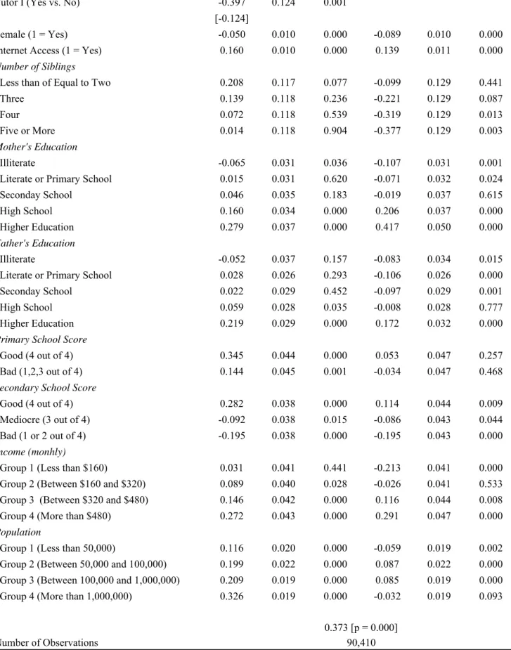
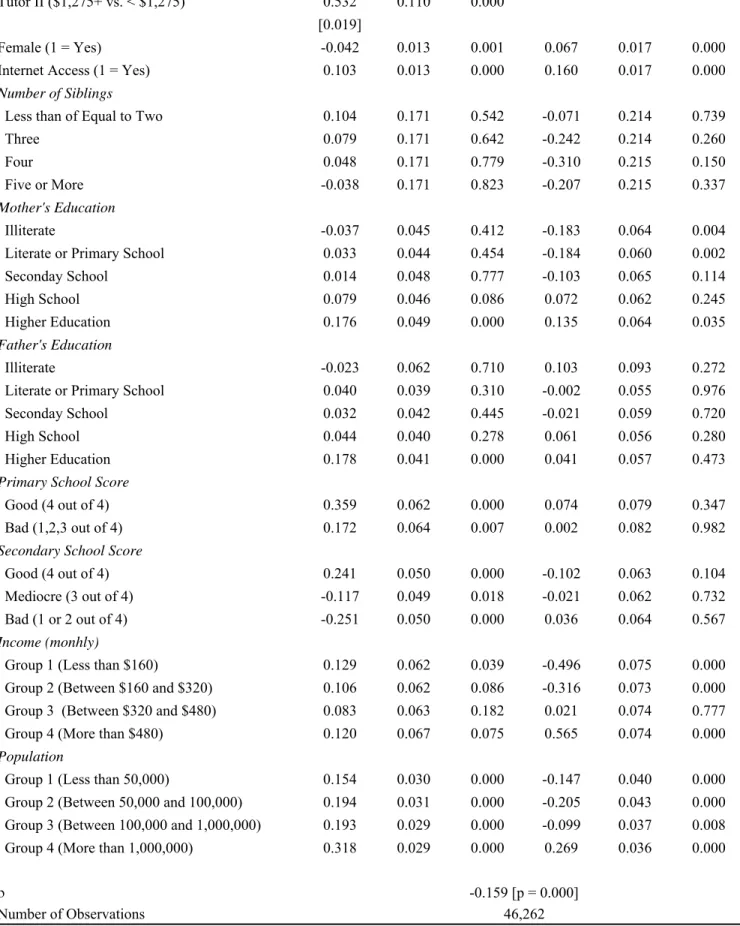
However, as Tables 3 and 4 indicate, the unconstrained bivariate probit results suggest a sizeable amount of non-random selection. Interestingly, though, the pattern di¤ers across the two treatments. In Table 3, we …nd strong evidence of positive selection into the Tutor I treatment (_b= 0:373, p= 0:000). Among students receiving private tutoring, Table 4 reveals evidence of negative selection into theTutor II treatment (_b = 0:159, p = 0:000). Thus, while unobservables associated with a higher likelihood of university placement arepositivelycorrelated with unobservables determining the use ofany private tutoring services, unobservables associated with a higher likelihood of university placement are negatively correlated with unobservables determiningexpenditures on private tutoring services (conditional on positive expenditures). In other words, there is positive selection into tutoring overall, but among students receiving tutoring, there is negative selection into high expenditures on tutoring.

Prior to assessing the impact of this selection on our ability to interpret the estimates obtained under selection on only observables in a causal manner, a brief examination of the remaining coe¢ cient estimates in Tables 3 and 4 is informative. In terms of explaining treatment assignment, we …nd that many of the variables are highly statistically signi…cant predictors of both treatments. First, as expected given our discussion in the Introduction, students from more a- uent households as measured family income, internet access, parental education, and fewer siblings are more likely to utilize private tutoring. In addition, conditional on positive expenditures, expenditures are increasing with internet access, mother’s education, and family income. Second, high expenditure on private tutoring (conditional on positive expenditures), and any tutoring to a lesser extent, are more common in larger, urban environments. Third, females are less likely to receive any private tutoring. However, conditional on receiving some private tutoring, households are more likely to spend greater amounts on tutoring for females. Finally, while tutoring and tutoring expenditures are unrelated to primary school test score, students scoring better on the secondary school test are more likely to receive tutoring prior to the university placement exam; secondary school test score is unrelated to expenditures conditional on receiving tutoring. Given these patterns, if private tutoring matters for university placement, policymakers and researchers ought to be concerned about the equity implications –particularly along economic and gender lines –of a large-scale tutoring system in Turkey.

positiveselection into theTutor I treatment in Panel I of Table 2. While the unconstrained estimates yield an estimate of_b= 0:373, the constrained results indicate that even a more modest amount of positive selection on unobservables is su¢ cient to eliminate and even reverse the sign of the treatment e¤ect. Speci…cally, when = 0:10, the estimated treatment e¤ect is reduced by over 60% (_b= 0:106, s.e. = 0:013), although the marginal e¤ect is unchanged (ME = 0.072). Setting = 0:20, we …nd a negative and statistically signi…cant e¤ect of tutoring on university placement (_b= 0:075, s.e. = 0:013; ME = -0.022). In the unconstrained estimation, = 0:373 and the treatment e¤ect falls to -0.397 (s.e. = 0:124); the ME is -0.124. In light of these results, we conclude that the causal e¤ect of any tutoring (versus no tutoring at all) is not robust, and admitting even modest levels of positive selection into tutoring is su¢ cient to conclude that private tutoring has a negligible or even a deleterious causal e¤ect on university placement.

Panel II of Table 2 assesses the implications of varying degrees of negative selection into the Tutor II

treatment. Given the positive coe¢ cient obtained when is constrained to zero, the e¤ect only becomes larger when one allows for negative selection. In the unconstrained estimation, = 0:158and the treatment e¤ect rises to 0.532 (s.e. = 0:110), implying a ME of 0.019. Thus, in contrast to Panel I, we …nd – among those utilizing private tutoring – greater expenditures on tutoring have a positive and robust causal e¤ect on university placement, although the magnitude is perhaps not overly large.

Combining the two sets of results, along with the summary statistics, indicates that the majority of students utilize tutoring, but spend less than $1,275 US dollars. Purchasing relatively low cost or short-term tutoring, however, at best has no impact on the probability of university placement, and at worst reduces the probability. However, for the small minority of students who use tutoring more intensively and/or purchase relatively expensive tutoring, such tutoring improves the probability of university placement. Since students from wealthy households with well-educated mothers are the primary recipients of large expenditures on private tutoring, the equity implications discussed previously are magni…ed. We now turn to the semi-nonparametric methods to see if this …nding continues to hold.

3.2

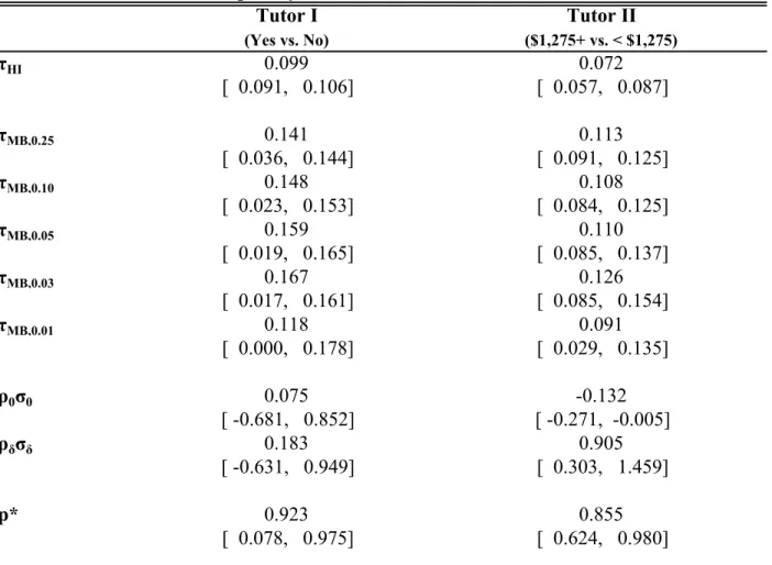
Propensity Score-Based Estimates

Table 5 presents the results obtained using the Hirano and Imbens (2001) weighting estimator. In terms of the …rst treatment, Tutor I, the Hirano and Imbens estimator applied to the entire sample indicates that tutoring is associated with a statistically signi…cant 10% increase in the probability of university placement ( HI = 0:099). However, minimizing the bias by restricting the sample to one percent of the treatment and control groups around the estimated bias-minimizing propensity score,p , of 0.923 increases the point estimate in contrast to our expectation from the parametric results ( M B;0:01= 0:118). However, the e¤ect

is only marginally statistically signi…cant as the 90% con…dence level just excludes zero. While the lack of statistical signi…cance may partly re‡ect the reduction in sample size, the estimation sample still includes

nearly 2,000 students. Lastly, the Heckman BVN results are consonant with the pattern of selection discussed previously, although the estimated coe¢ cients on the selection terms are not statistically signi…cant.

In terms of the second treatment, Tutor II, the Hirano and Imbens estimator applied to the entire sample indicates that tutoring is associated with a statistically signi…cant 7% increase in the probability of university placement ( HI = 0:072). However, minimizing the bias by restricting the sample to one percent of the treatment and control groups around the estimated bias-minimizing propensity score of 0.855 increases the estimate ( M B;0:01 = 0:091), and the e¤ect remains statistically signi…cant. In addition, the

Heckman BVN results indicate positive and statistically signi…cant selection into treatment on the basis of individual-speci…c, unobserved gains from treatment, but negative and statistically signi…cant selection on the basis of unobservables that a¤ect university placement absent the treatment. This pattern suggests that, ceteris paribus, students with a lower probability of university placement absent large expenditures on private tutoring, but who bene…t the most from such large expenditures, are more likely to spend a large amount on tutoring. Overall, the minimum bias approach applied to theTutor II treatment indicates, as in the parametric approach, that negative selection overall biases down the estimated treatment e¤ect.

3.2.2 Matching Estimates

Table 6 presents the …nal estimates, obtained utilizing kernel matching and Rosenbaum bounds. Panel I reveals a statistically signi…cant, estimated ATE of theTutor I treatment of 8% ( = 0:084), similar to the point estimate of the weighting estimator obtained under CIA. However, the Rosenbaum bounds reveal the lack of robustness of this estimate. Under a modest amount of positive selection on unobservables – such that observationally identical students di¤er in their relative odds of treatment by a factor of roughly 1.5, we fail to reject the null that the ATE is zero. Panel II reveals a statistically signi…cant, estimated ATE of theTutor II treatment of 9% ( = 0:093). Again, this is similar, as expected, to the point estimate of the weighting estimator obtained under CIA. Since negative selection only serves to strengthen the bene…cial e¤ect of greater spending, conditional on receiving any tutoring, the Rosenbaum bounds are uninformative in this case; they simply indicate that we continue to reject the null that the ATE is zero as we allow for increasingly strong negative selection.

3.3

Further Analysis

To assess the robustness of our conclusions, we perform two sets of additional analyses.8 _{First, we re-visit the} issue of non-random missing data for theTutor II treatment. Ideally one would have an exclusion restriction – a variable impacting the probability of having non-missing data that does not impact the probability of university placement conditional on the remaining regressors –enabling the estimation of Heckman selection model. However, such a variable is unlikely to exist in our data. Nonetheless, to get an idea of how the missing data impacts our results, we assume that all students who report utilizing some tutoring, but with

missing data on the exact amount spent on tutoring, spent less than $1,275 US dollars. In other words, we replace missing values for Tutor II with zero. As discussed above, since students with missing data come from less a- uent households in more rural areas, and these attributes are negatively associated with expenditures in Table 4, replacing missing values with zero may not be far o¤ the mark.

Proceeding along these lines, we repeat all of the previous estimations. In the interest of brevity, we simply summarize the results. First, the bivariate probit results, conditional on , are qualitatively unchanged. However, the unconstrained bivariate probit model yields _b = 0:006 (p= 0:904), indicating a failure to reject exogeneity. Under the assumption of exogeneity, the treatment e¤ect is_b= 0:278(s.e. = 0:019; ME = 0.005), which is similar to the estimate under exogeneity in Panel II of Table 2.

Second, the semi-nonparametric results replacing missing values ofTutor II with zero are also essentially unchanged. If anything, the estimates indicate a slightly larger impact of high expenditures on university placement. In sum, assuming that individuals with missing data spent less than $1,275 US dollars does not alter our conclusion that high spending on private tutoring has a bene…cial causal e¤ect on university placement conditional on using any tutoring.

Our second set of additional analyses allows the impact of private tutoring to di¤er along observable dimensions. Speci…cally, we repeat the previous analysis – of both the Tutor I and Tutor II treatments – for di¤erent sub-groups of students. First, we split the sample along gender lines. Second, we divided the sample into those with internet access and those without. Our conclusions regarding the impact of private tutoring did not qualitatively di¤er along these dimensions.

4

Conclusion

In this paper, we study the determinants and impacts of private tutoring in Turkey using a unique cross-sectional survey from 2002. Given our prior belief that selection into tutoring is non-random, but lacking a valid exclusion restriction, we employ recently developed estimation techniques from the program evaluation literature that assess the sensitivity of estimates obtained under conditional independence to selection on unobservables. Our results are striking, and should provide cause for alarm by policymakers already wary of the burgeoning market for private tutoring. Speci…cally, we reach three conclusions. First, while the use of private tutoring is positively associated with university placement, this appears entirely explained by positive selection. Moreover, allowing for even a modest amount of positive selection on unobservables indicates that, on average, tutoring actually decreases the probability of university placement. Second, there is a robust, positive causal e¤ect of tutoring –among those utilizing tutoring –on the probability of university placement if students spend a relatively large amount on tutoring (in excess of $1,275 US dollars). In combination, then, the results suggest that unless one is willing to invest heavily in private tutoring, one is better o¤ forsaking any tutoring. Finally, we …nd that the present utilization of private tutoring has potentially large implications on intergenerational income mobility and regional income disparities in Turkey. While tutoring

in general is extremely prevalent in Turkey, only the a- uent residing in major urban areas are likely to spend su¢ ciently to reap the rewards.

References

[1] Altonji, J.G., T.E. Elder, and C.R. Taber (2005), “Selection on Observed and Unobserved Variables: Assessing the E¤ectiveness of Catholic Schools,”Journal of Political Economy, 113, 151-184.

[2] Altonji, J.G., T.E. Elder, and C.R. Taber (2008), “Using Selection on Observed Variables to Assess Bias from Unobservables when Evaluating Swan-Ganz Catheterization,”American Economic Review, 98, 345-350.

[3] Aurini, J. and S. Davies (2003), “The Transformation of Private Tutoring: Education in a Franchise Form.” Submission for the Annual Meetings of the CSAA Halifax.

[4] Black, D.A. and J.A. Smith (2004), “How Robust is the Evidence on the E¤ects of College Quality? Evidence from Matching,”Journal of Econometrics, 121, 99-124.

[5] Bray, M. (1999), “The Shadow Education System: Private Tutoring and Its Implications for Planners,” Fundamentals of Educational Planning No. 61, Paris: UNESCO International Institute for Educational Planning (IIEP).

[6] Bray, M. and P. Kwok (2003), “Demand for Private Supplementary Tutoring: Conceptual Considera-tions and Socio-Economic Patterns.”Economics of Education Review, 22, 611-620.

[7] Dang, H.-A. (2007a), “The Determinants and Impact of Private Tutoring Classes in Vietnam,” unpub-lished Ph.D. dissertation, University of Minnesota.

[8] Dang, H.A. (2007b), “The Determinants and Impact of Private Tutoring Classes in Vietnam,” Eco-nomics of Education Review, 26, 684-699.

[9] Dang, H.A. and D. Halsey Rogers (2008), “How to Interpret the Growing Phenomenon of Private Tutoring: Human Capital Deepening, Inequality Increasing or Waster of Resources?” Policy Research Working Paper, World Bank.

[10] Ferraro, P.J., C. McIntosh, and M. Ospina (2007), “The E¤ectiveness of the US Endangered Species Act: An Econometric Analysis Using Matching Methods,”Journal of Environmental Economics and Management, 54, 245-261.

[11] Fisher, R.A. (1935),The Design of Experiments, Edinburgh: Oliver & Boyd.

[12] Hirano, K. and Imbens, G.W. (2001), “Estimation of Causal E¤ects using Propensity Score Weight-ing: An Application to Data on Right Heart Catheterization,”Health Services and Outcomes Research Methodology, 2, 259-278.

[13] Kang, C. (2007), “Does Money Matter? The E¤ect of Private Educational Expenditures on Academic Performance,” National University of Singapore, Department of Economics Working Paper No. 0704.

[14] Kim. S. and J.-H. Lee (2004), “Private Tutoring and Demand for Education in South Korea,” unpub-lished manuscript, University of Wisconsin-Milwaukee.

[15] Millimet, D.L. and R. Tchernis (2008), “Minimizing Bias in Selection on Observables Estimators when Unconfoundedness Fails,” unpublished manuscript, Southern Methodist University.

[16] Neyman, J. (1923), “On the Application of Probability Theory to Agricultural Experiments. Essay on Principles. Section 9,” translated inStatistical Science, (with discussion), 5, 465-480, (1990).

[17] Rosenbaum, P.R. (2002),Observational Studies, Second Edition. New York: Springer.

[18] Roy, A.D. (1951), “Some Thoughts on the Distribution of Income,”Oxford Economic Papers, 3, 135-146. [19] Rubin, D. (1974), “Estimating Causal E¤ects of Treatments in Randomized and Non-randomized

Stud-ies,”Journal of Educational Psychology, 66, 688-701.

[20] Stevenson, D.L. and D.P. Baker (1992), “Shadow Education and Allocation in Formal Schooling: Tran-sition to University in Japan,”American Journal of Sociology, 97, 1639-57

[21] Tansel, A. and F. Bircan (2005), “E¤ect of Private Tutoring on University Entrance Examination Performance in Turkey,” IZA Discussion Paper No. 1609.

[22] Tansel, A. and F. Bircan (2006), “Demand for Education in Turkey: A Tobit Analysis of Private Tutoring Expenditures,”Economics of Education Review, 25, 303-313.

[23] Tansel, A. and F. Bircan (2008), “Private Supplementary Tutoring in Turkey: Recent Evidence on Its Various Aspects,” IZA Discussion Paper No. 3471.

Table 1. Summary Statistics

Variable

N

Mean

SD

N

Mean

SD

N

Mean

SD

Diff

P-value

University Placement 90,410 0.280 0.449 26,124 0.212 0.409 46,262 0.364 0.481 -0.151 0.000 (1 = Yes) Tutor I (1 = Yes) 90,410 0.801 0.400 26,124 1.000 0.000 46,262 1.000 0.000 Tutor II (1 = $1,275+ 46,262 0.131 0.337 46,262 0.131 0.337 US dollars, 0 = between $1 and $1,275 US dollars) Female (1 = Yes) 90,410 0.451 0.498 26,124 0.433 0.495 46,262 0.457 0.498 -0.024 0.000 Internet Access (1 = Yes) 90,410 0.379 0.485 26,124 0.300 0.458 46,262 0.467 0.499 -0.167 0.000

Number of Siblings

Less than or Equal to Two 90,410 0.320 0.467 26,124 0.215 0.411 46,262 0.428 0.495 -0.213 0.000 Three 90,410 0.266 0.442 26,124 0.259 0.438 46,262 0.275 0.446 -0.015 0.000 Four 90,410 0.163 0.370 26,124 0.193 0.394 46,262 0.134 0.341 0.059 0.000 Five or More 90,410 0.249 0.432 26,124 0.330 0.470 46,262 0.163 0.369 0.168 0.000

Mother's Education

Illiterate 90,410 0.188 0.390 26,124 0.256 0.436 46,262 0.118 0.322 0.138 0.000 Literate or Primary School 90,410 0.525 0.499 26,124 0.563 0.496 46,262 0.482 0.500 0.080 0.000 Seconday School 90,410 0.065 0.247 26,124 0.050 0.217 46,262 0.079 0.270 -0.030 0.000 High School 90,410 0.109 0.312 26,124 0.056 0.229 46,262 0.165 0.371 -0.109 0.000 Higher Education 90,410 0.055 0.229 26,124 0.020 0.140 46,262 0.094 0.292 -0.074 0.000

Father's Education

Illiterate 90,410 0.034 0.180 26,124 0.051 0.219 46,262 0.018 0.131 0.033 0.000 Literate or Primary School 90,410 0.427 0.495 26,124 0.513 0.500 46,262 0.335 0.472 0.177 0.000 Seconday School 90,410 0.125 0.330 26,124 0.129 0.335 46,262 0.118 0.323 0.010 0.000 High School 90,410 0.181 0.385 26,124 0.140 0.347 46,262 0.221 0.415 -0.081 0.000 Higher Education 90,410 0.149 0.356 26,124 0.076 0.265 46,262 0.227 0.419 -0.151 0.000

Primary School Score

Good (4 out of 4) 90,410 0.715 0.451 26,124 0.624 0.484 46,262 0.800 0.400 -0.176 0.000 Bad (1,2,3 out of 4) 90,410 0.254 0.435 26,124 0.328 0.470 46,262 0.179 0.383 0.150 0.000

Secondary School Score

Good (4 out of 4) 90,410 0.235 0.424 26,124 0.165 0.371 46,262 0.303 0.460 -0.138 0.000 Mediocre (3 out of 4) 90,410 0.450 0.497 26,124 0.444 0.497 46,262 0.449 0.497 -0.006 0.149 Bad (1 or 2 out of 4) 90,410 0.275 0.447 26,124 0.337 0.473 46,262 0.215 0.411 0.122 0.000

Income (monhly)

Group 1 (Less than $160) 90,410 0.249 0.432 26,124 0.297 0.457 46,262 0.198 0.398 0.099 0.000 Group 2 (Between $160 90,410 0.117 0.322 26,124 0.102 0.303 46,262 0.129 0.336 -0.027 0.000 and $320)

Group 3 (Between $320 90,410 0.253 0.435 26,124 0.216 0.411 46,262 0.284 0.451 -0.068 0.000 and $480)

Group 4 (More than $480) 90,410 0.296 0.457 26,124 0.266 0.442 46,262 0.328 0.469 -0.062 0.000

Population

Group 1 (Less than 50,000) 90,410 0.385 0.487 26,124 0.486 0.500 46,262 0.270 0.444 0.216 0.000 Group 2 (Between 50,000 90,410 0.398 0.489 26,124 0.377 0.485 46,262 0.425 0.494 -0.047 0.000 and 100,000)

Group 3 (Between 100,000 90,410 0.120 0.325 26,124 0.077 0.267 46,262 0.165 0.371 -0.088 0.000 and 1,000,000)

Group 4 (More than 1,000,000) 90,410 0.083 0.275 26,124 0.037 0.190 46,262 0.130 0.336 -0.093 0.000

Table 2. Constrained Bivariate Probit Results

Panel I.

ρ = 0.00

ρ = 0.10

ρ = 0.20

ρ = 0.30

ρ = 0.40

ρ = 0.50

Tutor I

0.282

0.106

-0.075

-0.260

-0.449

-0.643

(0.013)

(0.013)

(0.013)

(0.012)

(0.012)

(0.012)

[0.072]

[0.072]

[-0.022]

[-0.078]

[-0.142]

[-0.211]

Panel II.

ρ = 0.00

ρ = -0.10

ρ = -0.20

ρ = -0.30

ρ = -0.40

ρ = -0.50

Tutor II

0.248

0.430

0.612

0.793

0.972

1.150

(More than $1,275 vs. Less than $1,275)

(0.019)

(0.019)

(0.019)

(0.019)

(0.018)

(0.018)

[0.009]

[0.015]

[0.021]

[0.026]

[0.029]

[0.033]

Coefficient

(Standard Error)

Table 3. Unconstrained Bivariate Probit Results: Tutor I Treatment

Coeff

S.E.

P-value

Coeff

S.E.

P-value

Tutor I (Yes vs. No) -0.397 0.124 0.001

[-0.124]

Female (1 = Yes) -0.050 0.010 0.000 -0.089 0.010 0.000

Internet Access (1 = Yes) 0.160 0.010 0.000 0.139 0.011 0.000

Number of Siblings

Less than of Equal to Two 0.208 0.117 0.077 -0.099 0.129 0.441

Three 0.139 0.118 0.236 -0.221 0.129 0.087

Four 0.072 0.118 0.539 -0.319 0.129 0.013

Five or More 0.014 0.118 0.904 -0.377 0.129 0.003

Mother's Education

Illiterate -0.065 0.031 0.036 -0.107 0.031 0.001

Literate or Primary School 0.015 0.031 0.620 -0.071 0.032 0.024

Seconday School 0.046 0.035 0.183 -0.019 0.037 0.615

High School 0.160 0.034 0.000 0.206 0.037 0.000

Higher Education 0.279 0.037 0.000 0.417 0.050 0.000

Father's Education

Illiterate -0.052 0.037 0.157 -0.083 0.034 0.015

Literate or Primary School 0.028 0.026 0.293 -0.106 0.026 0.000

Seconday School 0.022 0.029 0.452 -0.097 0.029 0.001

High School 0.059 0.028 0.035 -0.008 0.028 0.777

Higher Education 0.219 0.029 0.000 0.172 0.032 0.000

Primary School Score

Good (4 out of 4) 0.345 0.044 0.000 0.053 0.047 0.257

Bad (1,2,3 out of 4) 0.144 0.045 0.001 -0.034 0.047 0.468

Secondary School Score

Good (4 out of 4) 0.282 0.038 0.000 0.114 0.044 0.009

Mediocre (3 out of 4) -0.092 0.038 0.015 -0.086 0.043 0.044

Bad (1 or 2 out of 4) -0.195 0.038 0.000 -0.195 0.043 0.000

Income (monhly)

Group 1 (Less than $160) 0.031 0.041 0.441 -0.213 0.041 0.000

Group 2 (Between $160 and $320) 0.089 0.040 0.028 -0.026 0.041 0.533

Group 3 (Between $320 and $480) 0.146 0.042 0.000 0.116 0.044 0.008

Group 4 (More than $480) 0.272 0.043 0.000 0.291 0.047 0.000

Population

Group 1 (Less than 50,000) 0.116 0.020 0.000 -0.059 0.019 0.002

Group 2 (Between 50,000 and 100,000) 0.199 0.022 0.000 0.087 0.022 0.000

Group 3 (Between 100,000 and 1,000,000) 0.209 0.019 0.000 0.085 0.019 0.000

Group 4 (More than 1,000,000) 0.326 0.019 0.000 -0.032 0.019 0.093

ρ

Number of Observations

Note: Tutor I treatment is one for students utilizing any private tutoring, zero otherwise. Marginal effect for treatment effect in brackets.

0.373 [p = 0.000] 90,410

Table 4. Unconstrained Bivariate Probit Results: Tutor II Treatment

Coeff

S.E.

P-value

Coeff

S.E.

P-value

Tutor II ($1,275+ vs. < $1,275) 0.532 0.110 0.000

[0.019]

Female (1 = Yes) -0.042 0.013 0.001 0.067 0.017 0.000

Internet Access (1 = Yes) 0.103 0.013 0.000 0.160 0.017 0.000

Number of Siblings

Less than of Equal to Two 0.104 0.171 0.542 -0.071 0.214 0.739

Three 0.079 0.171 0.642 -0.242 0.214 0.260

Four 0.048 0.171 0.779 -0.310 0.215 0.150

Five or More -0.038 0.171 0.823 -0.207 0.215 0.337

Mother's Education

Illiterate -0.037 0.045 0.412 -0.183 0.064 0.004

Literate or Primary School 0.033 0.044 0.454 -0.184 0.060 0.002

Seconday School 0.014 0.048 0.777 -0.103 0.065 0.114

High School 0.079 0.046 0.086 0.072 0.062 0.245

Higher Education 0.176 0.049 0.000 0.135 0.064 0.035

Father's Education

Illiterate -0.023 0.062 0.710 0.103 0.093 0.272

Literate or Primary School 0.040 0.039 0.310 -0.002 0.055 0.976

Seconday School 0.032 0.042 0.445 -0.021 0.059 0.720

High School 0.044 0.040 0.278 0.061 0.056 0.280

Higher Education 0.178 0.041 0.000 0.041 0.057 0.473

Primary School Score

Good (4 out of 4) 0.359 0.062 0.000 0.074 0.079 0.347

Bad (1,2,3 out of 4) 0.172 0.064 0.007 0.002 0.082 0.982

Secondary School Score

Good (4 out of 4) 0.241 0.050 0.000 -0.102 0.063 0.104

Mediocre (3 out of 4) -0.117 0.049 0.018 -0.021 0.062 0.732

Bad (1 or 2 out of 4) -0.251 0.050 0.000 0.036 0.064 0.567

Income (monhly)

Group 1 (Less than $160) 0.129 0.062 0.039 -0.496 0.075 0.000

Group 2 (Between $160 and $320) 0.106 0.062 0.086 -0.316 0.073 0.000

Group 3 (Between $320 and $480) 0.083 0.063 0.182 0.021 0.074 0.777

Group 4 (More than $480) 0.120 0.067 0.075 0.565 0.074 0.000

Population

Group 1 (Less than 50,000) 0.154 0.030 0.000 -0.147 0.040 0.000

Group 2 (Between 50,000 and 100,000) 0.194 0.031 0.000 -0.205 0.043 0.000

Group 3 (Between 100,000 and 1,000,000) 0.193 0.029 0.000 -0.099 0.037 0.008

Group 4 (More than 1,000,000) 0.318 0.029 0.000 0.269 0.036 0.000

ρ

Number of Observations 46,262

Outcome

Treatment Assignment

-0.159 [p = 0.000]

Table 5. Minimum Bias Propensity Score Results

Tutor I

Tutor II

τ

0.099

0.072

[ 0.091, 0.106]

[ 0.057, 0.087]

τ

0.141

0.113

[ 0.036, 0.144]

[ 0.091, 0.125]

τ

0.148

0.108

[ 0.023, 0.153]

[ 0.084, 0.125]

τ

0.159

0.110

[ 0.019, 0.165]

[ 0.085, 0.137]

τ

0.167

0.126

[ 0.017, 0.161]

[ 0.085, 0.154]

τ

0.118

0.091

[ 0.000, 0.178]

[ 0.029, 0.135]

ρ

σ

0.075

-0.132

[ -0.681, 0.852]

[ -0.271, -0.005]

ρ

σ

0.183

0.905

[ -0.631, 0.949]

[ 0.303, 1.459]

p*

0.923

0.855

[ 0.078, 0.975]

[ 0.624, 0.980]

Notes: 90% empirical confidence intervals obtained using 200 bootstrap repetitions. HI = Hirano and Imbens (2001) normalized estimator; MB = minimum biased estimator using θ = 0.25, 0.10, 0.05, 0.03, or 0.01. p* = bias-minimizing propensity score.

Table 6. Propensity Score (Kernel) Matching Estimates and Rosenbaum Bounds

ATE

Γ

= 1

Γ

= 1.2

Γ

= 1.4

Γ

= 1.6

Γ

= 1.8

Γ

= 2

Γ

= 2.5

Γ

= 3

Panel I.

Tutor I

0.084

p = 0.000 p = 0.000 p = 0.000 p = 0.948 p = 1.000 p = 1.000 p = 1.000 p = 1.000

[0.073, 0.095]

Panel II.

Tutor II

0.093

p = 0.000 p = 0.000 p = 0.000 p = 1.000 p = 1.000 p = 1.000 p = 1.000 p = 1.000

[0.075, 0.112]